HAL Id: hal-03120932
https://hal.archives-ouvertes.fr/hal-03120932
Submitted on 8 Feb 2021
HAL is a multi-disciplinary open access
archive for the deposit and dissemination of
sci-entific research documents, whether they are
pub-lished or not. The documents may come from
teaching and research institutions in France or
L’archive ouverte pluridisciplinaire HAL, est
destinée au dépôt et à la diffusion de documents
scientifiques de niveau recherche, publiés ou non,
émanant des établissements d’enseignement et de
recherche français ou étrangers, des laboratoires
rock magnetic and geochemical parameters in relation to
climate during the last 276 kyr in the Azores region
P. Kruiver, Y. Kok, M. Dekkers, C. Langereis, C. Laj
To cite this version:
P. Kruiver, Y. Kok, M. Dekkers, C. Langereis, C. Laj. A pseudo-Thellier relative palaeointensity
record, and rock magnetic and geochemical parameters in relation to climate during the last 276 kyr
in the Azores region. Geophysical Journal International, Oxford University Press (OUP), 1999, 136
(3), pp.757-770. �10.1046/j.1365-246x.1999.00777.x�. �hal-03120932�
A pseudo-Thellier relative palaeointensity record, and rock magnetic
and geochemical parameters in relation to climate during the last
276 kyr in the Azores region
P. P. Kruiver,1 Y. S. Kok,1 M. J. Dekkers,1 C. G. Langereis1 and C. Laj2
1 Utrecht University, Faculty of Earth Sciences, Palaeomagnetic L aboratory ‘Fort Hoofddijk’, Budapestlaan 17, 3584 CD Utrecht, the Netherlands 2 L aboratoire des Sciences du Climat et de l’Environnement (L SCE), Campus du CNRS, Avenue de la T errasse, 91198 Gif-sur-Yvette, France
Accepted 1998 November 16. Received 1998 August 17; in original form 1998 January 12
S U M M A R Y
In the pseudo-Thellier method for relative palaeointensity determinations (Tauxe et al. 1995) the slope of the NRM intensity left after AF demagnetization versus ARM intensity gained at the same peak field is used as a palaeointensity measure. We tested this method on a marine core from the Azores, spanning the last 276 kyr. We compared the pseudo-Thellier palaeointensity record with the conventional record obtained earlier by Lehman et al. (1996), who normalized NRM by SIRM. The two records show similar features: intensity lows with deviating palaeomagnetic directions at 40–45 ka and at 180–190 ka. The first interval is associated with the Laschamps excursion, while the 180–190 ka low represents the Iceland Basin excursion (Channell et al. 1997). The pseudo-Thellier method, in combination with a jackknife resampling scheme, provides error estimates on the palaeointensity.
Spectral analysis of the rock magnetic parameters and the palaeointensity estimates shows orbitally forced periods, particularly 23 kyr for climatic precession. This suggests that palaeointensity is still slightly contaminated by climate. Fuzzy c-means cluster analysis of rock magnetic and geochemical parameters yields a seven-cluster model of predominantly calcareous clusters and detrital clusters. The clusters show a strong correlation with climate, for example samples from detrital clusters predominantly appear during rapid warming. Although both the pseudo-Thellier palaeointensity m
a and fuzzy clusters show climatic influences, we have not been able to find an unambiguous connection between the clusters and m
a.
Key words: climate, fuzzy cluster analysis, pseudo-Thellier, relative palaeointensity,
rock magnetism.
mation from the NRM signal is by performing a normalization 1 I N T R O D U C T I O N
of the NRM intensities by some normalizer. This normalizer A knowledge of geomagnetic intensity variations is crucial to should account for changes in magnetic grain size and concen-the understanding of concen-the geodynamo. In addition, concen-the geo- tration, which also affect the strength of the NRM signal. magnetic field strength is believed to modulate the10Be and Different normalizers have been proposed such as saturation 14C production by shielding cosmic rays and thus influencing isothermal remanent magnetization (SIRM), anhysteretic ages obtained by14C dating (for example Raisbeck et al. 1987; remanent magnetization (ARM) and magnetic susceptibilityk Bard et al. 1990; Mazaud et al. 1991; Robinson et al. 1995). (see Tauxe 1993). The palaeointensity would be represented by Many efforts have been made to recover the palaeointensity for example NRM
25mT/ARM25mT. Similarity between normalized from sedimentary records. Principally, sedimentary sequences records obtained by different normalizers, and dissimilarity offer continuous high-resolution records of the natural remanent between normalized and non-normalized records are often magnetization (NRM). The NRM contains information about believed to express the reliability of the palaeointensity record. the geomagnetic field at or shortly after the time of deposition Normalizing the record is assumed to minimize the effects of of the sediment. However, the processes by which the sediments magnetic grain-size distribution and variation of magnetic acquire their NRM are still not known in sufficient detail. The input, for example determined by climate. Criteria for choosing the magnetic material used in palaeointensity estimates from conventional method of extracting geomagnetic field
sedimentary sequences are summarized by Tauxe (1993). It is based on dating by Lehman et al. (1996) using thed18O record from the same core, which was correlated to the oxygen only possible to obtain a relative palaeointensity estimate from
sediments in this way, in contrast to the absolute palaeointensity isotopic record of Martinson et al. (1987).
Individual samples were taken by inserting 8 cm3 perspex determinations from lavas and igneous rocks.
Many palaeointensity records have been published recently cylinders in the core at approximately 5 cm intervals for k measurements and at 10 cm intervals for NRM and ARM (e.g. Meynadier et al. 1992; Valet & Meynadier 1993; Weeks
et al. 1995; Channell et al. 1997). Each study argues that their measurements, corresponding to average resolutions of 1450 and 2900 yr, respectively. Sample numbers correspond to records represent the true geomagnetic field intensity and are
free of environmental influences. It is recognized, however, that depths (in cm) in the core.
The magnetic susceptibility was measured with a low-field the sedimentary palaeointensity record might still be biased
by environmentally caused variations in magnetic grain size magnetic susceptibility bridge KLY2 instrument. NRM and ARM were measured with a vertical 2G RF SQUID cryo-and concentration (e.g. Schwartz et al. 1996). Although the
criteria summarized by Tauxe (1993) are strict, one must be genic magnetometer (noise level 10−11 Am2) in a magnetically shielded room or with a horizontal 2G DC SQUID cryogenic aware that there might still be some climate influence left in
the normalized NRM record and that we might not be looking magnetometer (noise level 3×10⁻¹² Am2). IRM was measured on a JR5 A spinner magnetometer (noise level 5×10⁻¹¹ Am2). at a purely geomagnetic signal.
Recently, two new methods have been proposed to recover Comparison with measurements on the SQUID magneto-meters showed that spinning of the moist samples in the palaeointensity from sediments: the pseudo-Thellier method,
based on AF demagnetization and ARM (or IRM) acquisition spinner magnetometer did not affect the measurements. Palaeointensity determinations were performed according (Tauxe et al. 1995), and a Thellier–Thellier method for
sediments, based on thermal demagnetization of the NRM and to Tauxe et al. (1995) with the pseudo-Thellier method using ARM on 117 samples. We use ARM and not IRM acquisition acquisition of a partial thermoremanent magnetization
(pTRM) (Hartl & Tauxe 1996). It has been argued that these because Tauxe et al. (1995) showed that the plot of ARM left versus ARM gained at the same peak field is somewhat linear, new methods diminish the environmental contamination of the
palaeointensity signal better than the conventional normalizing whereas IRM left versus IRM gained is markedly curved. The pseudo-Thellier method is illustrated in Fig. 1. First, methods. The pseudo-Thellier and the conventional method
gave significantly different results for samples from the the NRM is demagnetized by means of alternating fields (AF) in 14 steps up to 125 mT using steps of 5–25 mT Ongtong-Java Plateau (Tauxe et al. 1995), whereas similar
results were obtained for samples from Hole 851C (Pacific (Fig. 1a). An ARM is then imparted at the same field steps as the NRM demagnetization. ARM
max indicates the ARM Ocean) and core MD90–0940 (Indian Ocean) by Valet &
Meynadier (1998). Here, we compare the pseudo-Thellier intensity acquired at 125 mT. The bias field was 45 mT in the direction perpendicular to the axis of the coil. Initial method with ARM and the conventional normalizing method
on a core spanning the last 276 kyr which seemed to have an NRM intensities typically range from 5–300 mA m−1 (average 52±44 mA m−1) and ARM
maxintensities from 70–800 mA m−1 excellent conventional palaeointensity record (Lehman et al.
1996). The aim of this paper is to investigate whether the (average 198±125 mA m−1). The average median destructive field (MDF) for the NRM is 25±4 mT. If we plot the NRM pseudo-Thellier method yields different results for this core. It
is important to perform such a check on a core which is likely intensity left after demagnetization versus the acquired ARM intensity (at the same peak fields, Fig. 1b) we can determine to have suffered little diagenetic alteration. Lehman et al.
(1996) studied several marine sedimentary cores from the the best-fit slope, m
a(where ‘a’ stands for ARM), with linear regression and an error estimate using a jackknife resampling Azores area, using the method of normalizing NRM by SIRM
and ARM and continuous U-channel measurements. They procedure (Efron 1982; Kok et al. 1998). The jackknife resampling procedure calculates the slope through every concluded that the cores were very suitable for palaeointensity
determination. In this study, we determine the palaeointensity possible combination of at least four data points, starting at fields higher than 35 mT; 90 per cent of these slope values lie from one of these cores (SU92–18, spanning the last 276 kyr)
with the pseudo-Thellier method and with the conventional between the dashed lines in Fig. 1(c), giving an upper and lower limit for ma. We used 35 mT field steps and higher, method, both on discrete samples. In addition, whole-rock
geochemical analyses are carried out to study the environ- because the NRM left at lower steps might still be suffering from a viscous overprint. The value of m
agiven in Fig. 1(b) mental influences on the sediments in this core. Finally, fuzzy
c-means cluster analysis on rock magnetic and geochemical corresponds to the slope with the smallest relative error of NRM left versus ARM gained through at least four successive parameters is performed. It provides a method of studying
the relationships between rock magnetic parameters and the data points (solid line in histogram of Fig. 1c).
The determination of ma with the pseudo-Thellier method geochemical environment (Dekkers et al. 1994).
in combination with the jackknife resampling procedure is based on a linear relationship between ARM gained and ARM 2 M AT E R I A L S AN D M E T H OD S
left at the same field steps (Tauxe et al. 1995). To check this relationship, the ARM
max of nine samples, selected to have a The core investigated in this study is core SU92–18 from the
Azores area (37°47∞3◊N, 27°13∞9◊W), north Atlantic Ocean. It wide range of initial ARM intensities, was AF demagnetized in three perpendicular directions at the same field steps as is 9.93 m long and was taken from a water depth of 2300 m.
The lithology seems rather homogeneous and is dominated by the ARM acquisition. This was done for the DC bias field perpendicular and parallel to the AF direction (Fig. 2). The nannofossil ooze with clay minerals and volcanic products. A
tephra layer is situated between 582 and 605 cm depth (Lehman relationship is not linear for the ‘perpendicular’ ARM: the samples are more easily demagnetized than magnetized, et al. 1996). The average sedimentation rate was 3.5 cm kyr−1
(a)
(b) (c)
Figure 2. (a) Example of difference between ‘perpendicular’ and
‘parallel’ ARM acquisition. For parallel ARM acquisition the DC bias field was 30 mT and parallel to the AF field direction (triangles). For
(a)
(b)
(c)
perpendicular ARM the DC bias field was 45 mT and perpendicular
Figure 1. Pseudo-Thellier method for sample 200. (a) Stepwise AF to the AF field direction (squares). Demagnetization of the ARM is demagnetization of NRM and (corrected) acquisition of ARM; intensities also shown. (b) Average curve of nine samples of normalized ARM are normalized by their maximum values, initial NRM intensity is left after demagnetization versus ARM gained at the same field steps 55.5 mA m−1, maximum ARM intensity is 120.5 mA m−1. (b) NRM for perpendicular ARM acquisition. Field steps (from upper left to intensity left after demagnetization to a given peak field versus ARM lower right): 0, 5, 10, 15, 20, 25, 30, 35, 40, 50, 60, 70, 80, 100 and intensity gained at the same peak field. The best-fit slope through 125 mT. Maximum ARM intensities range from 73–826 mA m−1. The at least four successive data points is palaeointensity estimate m
a curve is markedly bent. (c) As ( b) for parallel ARM acquisition. The (solid line in c); other possible values for the slope are determined with curve is nearly linear. For the determination of the palaeointensity the jackknife resampling method, resulting in an upper and lower limit with the pseudo-Thellier method (Tauxe et al. 1995), the measured for ma; (c) histogram of possible ma values. Solid line: best-fit slope perpendicular ARM intensities are converted to parallel ARM intensities through at least four successive data points; dashed lines: upper and by multiplication with a correction factor determined from the average lower limits of 90 per cent of possible mavalues. Jackknife parameters: curves shown in (b) and (c).
n is the number of calculated slopes. Determination of slopes from fields of 35 mT and higher.
particularly at higher fields (Figs 2a and b). The ‘parallel’ ARM shows a nearly linear relationship (Figs 2a and c). The perpendicular ARM acquisition intensities are too low compared to parallel ARM acquisition intensities. Therefore, the perpendicular ARM acquisition intensities, which were measured for all samples, are corrected to parallel ARM acquisition intensities by multiplication with a correction factor derived from the set of nine samples. These corrected ARM intensities are then used in the pseudo-Thellier palaeointensity determination.
Figure 3. Comparison of palaeointensity estimates ma obtained with
To validate this correction, ma was calculated for both perpendicular ARM acquisition (circles) and parallel ARM acquisition
parallel and perpendicular ARMs for the nine samples (Fig. 3). (squares) for nine samples (see text). Vertical lines denote jackknife From this figure it is seen that the jackknife error for the errors at a 90 per cent confidence level. x-axis labels are sample ‘perpendicular’ ma is larger. This is because the NRM left versus numbers.
ARM gained plot is less linear than for the ‘parallel’ m a. In addition, the parallel m
a is always slightly higher than the IRM acquisition with subsequent AF and DC demagnetization perpendicular ma. The shape of the curve, however, remains was performed on eight samples to screen for possible magnetic unchanged and we conclude that our correction of perpendicular interaction (Henkel 1964; Cisowski 1981). IRM was imparted with a PM4 pulse magnetizer. Stepwise acquisition and ARMs to parallel ARMs is valid.
demagnetization were carried out up to fields of 250 mT for from the ‘low’-coercivity component; the latter component is removed in fields as high as 100 mT and thus can hardly be AF treatment and up to 800 mT for DC treatment. A
three-component IRM (Lowrie 1990) was thermally demagnetized. regarded as a viscous overprint.
Declinations and inclinations are shown in Fig. 5. For the Orthogonal IRM fields were 2.7 T, 500 mT and 80 mT. Curie
balance experiments on magnetic extracts have already been deviating demagnetization behaviour interval, both high- and ‘low’-coercivity components are plotted. The high-coercivity performed by Lehman et al. (1996). In the present study,
thermomagnetic runs were performed on selected samples with components are determined using the great-circles method (McFadden & McElhinny 1988) and they show directions a modified horizontal translation Curie balance, which uses a
sinusoidally cycling field instead of a steady field (Mullender comparable to the rest of the record. The ‘low’-coercivity components (removed at 80–100 mT) show directions that et al. 1993). The extraction of magnetic material was not
necessary for thermomagnetic analysis. deviate significantly. Also, in the interval around 40 ka we find deviating declinations and steep inclinations. This represents Geochemical data from 108 samples were obtained with
ICP-OES analysis (inductively coupled plasma optical emission the Laschamps excursion. The trend in declination at the very top of the core is probably caused by physical rotation during spectrometer, Perkin Elmer-type Optima 3000). The samples
were dried, crushed and ground to a powder. About 250 mg of coring. The difference in inclination between this study and that of Lehman et al. (1996) near 550–600 cm depth is likely to each sample was completely dissolved in a mixture of HF, HNO
3
and HClO4. The samples were heated overnight, evaporated to have been caused by the strongly magnetic tephra layer, which might disturb U-channel measurements and accompanying dryness and diluted with HCl and demineralized water for
analysis. Accuracy and precision were checked with laboratory deconvolution.
The results of the Curie balance measurements show that standards and duplicate analyses. The analytical error was
better than 5 per cent for Ca, Mn, Fe, Al, Ti, Zr, Ba and K the material consists predominantly of low-Ti magnetite with a Curie temperature of approximately 570°C (Fig. 6). Upon and better than 10 per cent for S.
Multivariate classification was carried out with fuzzy heating to 400°C the titanomagnetite is exsolved into pure magnetite and an end-member of ulvo¨spinel, resulting in a c-means cluster analysis (Bezdek 1981). This is a partitioning
method, in which n cases are divided into a number of clusters. slightly stronger magnetic phase. The irreversibility of the 400°C run is not severe, indicating a low Ti content. The Curie The best clustering for a certain number of clusters is calculated
by minimizing the distance between a sample and its cluster temperature of the exsolved magnetite is slightly lower than the Curie temperature of pure magnetite (580°C). A low-Ti centre and maximizing the distance between cluster centres.
The ‘fuzzy’ concept implies that a sample is not forced to fit magnetite is also indicated by the unblocking temperatures close to 580°C of the three-component IRM (see Lowrie 1990) into one particular cluster, but is assigned a membership to
each cluster. The membership ranges from 0 (no similarity in Fig. 7. The Curie balance measurements agree with those of Lehman et al. (1996). Their rock magnetic study shows that between sample and cluster) to 1 (identical ). The memberships
to the clusters for one sample add up to 1. A sample is called the grain size is fairly constant throughout the whole core. The hysteresis measurements show that the grain-size range is an intermediate case when the ratio of the largest but one
membership to the largest membership is more than 0.6. No small and that all samples fall within the pseudo-single-domain (PSD) range (Lehman et al. 1996). They also found a rather a priori information on the existence of grouping in the data
set is required. A more detailed description of the algorithm constant ARM25mT/k ratio, which is another indication of a mainly uniform grain size. Hence, to a first approximation, of fuzzy clustering is given in Kaufman & Rousseeuw (1990).
Fuzzy c-means clustering was applied to the following para- we consider variations in k, SIRM and ARM intensities as variations in concentration.k varies from 300–4500×10−6 SI meters:k, ARMmax, ARMmax/k, Ca, S, Mn, Fe/Al, Al, Ti, Zr,
Ba and K. The parameters are standardized before the fuzzy and SIRM intensities range from 12–45 Am−1.
From Fig. 2(c) it is seen that even the parallel ARM cluster algorithm is run to ascertain that all parameters have
equal weight. Also, parameters with log-normal distributions acquisition and demagnetization curve used for the pseudo-Thellier palaeointensity determination is not perfectly linear. (k, ARMmax, S, Mn, Fe/Al, Al, Ti, Ba, K) are logarithmically
transformed before standardization. A possible explanation for this is the existence of magnetic interaction. To screen for magnetic interaction, IRM acquisition curves and corresponding DC and AF demagnetization curves 3 R E S U LT S
were measured. The acquisition and DC demagnetization curves of IRM (Fig. 8a) show that a typical sample is saturated 3.1 Palaeomagnetic and rock magnetic results
at approximately 250 mT. If IRM gained is plotted versus IRM left (Fig. 8b) in a so-called Henkel plot (Henkel 1964), Almost all samples show the same NRM demagnetization
behaviour. Representative demagnetization diagrams show a the presence of magnetic interaction can be checked (Wohlfarth 1958). Non-linearity in the Henkel plot is usually attributed single-component NRM, which is demagnetized towards the
origin (Figs 4a and b). The NRM is often not completely to interparticle dipolar interactions in fine-particle systems (Cisowski 1981). Our results show curves that are concave up, removed after demagnetization at 125 mT. This implies a rather
high coercivity for magnetite, which is of PSD grain size which suggests that some positive magnetic interaction may occur (Fearon et al. 1990), although this may only pertain to (Lehman et al. 1996). The coercivity of magnetite, however, can
be considerably increased by low-temperature surface oxidation SD magnetite.
The results of IRM acquisition and subsequent AF (van Velzen & Zijderveld 1995). Deviating demagnetization
behaviour is detected in the depth interval 636–664 cm demagnetization (Fig. 8c) are similar for all samples, regardless of their maximum IRM intensity values. The point of inter-(corresponding to 180–190 ka, Figs 4c and d). These samples
contain a high-coercivity component with a direction different section of the acquisition and demagnetization curves is at
(a)
(b)
(c)
(d)
Figure 4. Zijderveld diagrams of typical samples. Solid (open) circles denote projections on the horizontal (vertical ) plane. Field steps are 0, 5,
10, 15, 20, 25, 30, 35, 40, 50, 60, 70, 80, 100 and 125 mT. (a) 200 cm depth, NRM
0=55.5 mA m−1; (b) 799 cm depth, NRM0=81.1 mA m−1. Zijderveld diagrams for the two-component NRM interval of depth 636–664 cm: (c) 639 cm depth, NRM
0=4.7 mA m−1; (d) 644 cm depth, NRM
0=6.0 mA m−1.
approximately 35 per cent of the maximum IRM intensity. magnetic particles consist of (low-Ti) magnetite. Thus, magnetic interaction may occur within a particle, such as is seen in Cisowski (1981) suggests that there is no magnetic interaction
if the point of intersection is at 50 per cent of the maximum bicompositional (Housden & O’Reilly 1990; van Velzen & Zijderveld 1995) or intergrown grains (e.g. de Boer & Dekkers IRM intensity. We note, however, that Cisowski (1981)
investi-gated magnetic interaction for SD particles and his results 1996), rather than between particles. The decrease in IRM intensity of all three induced components (Fig. 7) between 150 might not be applicable to the PSD particles in our samples.
It is unlikely, however, that magnetic interaction has played and 200°C also suggests surface oxidation of the magnetic grains (van Velzen & Zijderveld 1995).
a significant role in these sediments. First, it is striking that all samples show virtually the same behaviour in these IRM experiments, independent of the absolute IRM intensities. The
3.2 Palaeointensity estimates degree of interaction between magnetic particles is dependent
on concentration (e.g. Sugiura 1979; Banerjee & Mellema Lehman et al. (1996) showed that the magnetic material satisfies the criteria for palaeointensity determinations of Tauxe 1974). If the between-grain interaction was important, samples
with a relatively high concentration (i.e. high IRM intensity) (1993). Lehman et al. (1996) took NRM25mT/SIRM for the conventional palaeointensity estimate. We have taken NRM
25mT/ and samples with a low concentration ( low IRM intensity)
would behave differently. All samples deviate to the same ARM
maxas a conventional palaeointensity estimate because the pseudo-Thellier method uses ARM as well. Moreover, Lehman extent from the non-interaction line (slope−0.5) in the Henkel
plot. Moreover, the point of intersection in the Cisowski plot et al. (1996) showed that both normalizers give strikingly similar results. Both conventional palaeointensity records (approximately 35 per cent) is the same for all samples.
Second, for magnetic interaction to occur between grains, are shown in Fig. 9(a). In order to compare them they are both normalized by their mean values. In general, the two the concentration must be much higher (>0.1–1 per cent)
than is usually observed in sediments. In core SU92–18 the records agree well. The Lehman et al. (1996) record has a
Figure 7. Thermal demagnetization of three-component IRM (Lowrie
1990). Maximum IRM fields of 2.7 T, 500 mT and 80 mT were applied subsequently along three orthogonal directions for samples 160, 408, 616, 729, 819.
higher resolution than ours, because of continuous U-channel measurements.
The pseudo-Thellier palaeointensity ma is given in Fig. 9(b). Again the record is normalized by the mean, resulting in positive values for ma. The solid line represents the best-fit
Figure 5. Declination and inclination determined from AF demag- slope found with at least four successive data points. The shaded
netization. Declinations have been adjusted to obtain an average value area gives 90 per cent of all possible values of m
aaccording to
of 0°. Dashed horizontal lines indicate core boundaries. Dashed curve
the jackknife resampling method (see for explanation Fig. 1).
is from Lehman et al. (1996) (continuous U-channel measurements);
Comparing the conventional record and the pseudo-Thellier
solid line with solid symbols (discrete samples) is from this study.
record it is seen that both records show prominent intensity
Both hard (asterisks) and ‘soft’ (inverted triangles) components are
lows at 40–45 and 180–190 ka. From the declination and
plotted for the two-component NRM interval of 636–664 cm depth
inclination plot (Fig. 5) we conclude that the 40–45 ka low
(age 180–190 ka). Hard components have been determined using
great circles. corresponds to the Laschamps excursion (see Nowaczyk et al. 1994 and references therein). No deviating directions, however, are detected for the Blake excursion (110–120 ka). The 180–190 ka low-intensity interval corresponds to the 636–664 cm depth interval, which shows deviating NRM demagnetization behaviour, representing the Icelandic Basin reversal excursion at approximately 188 ka (Channell et al. 1997); this is discussed in Section 4.4. The high peak at about 170 ka is caused by a tephra layer. The values for NRM, ARM and IRM intensities of this layer are very different from the rest of the core. Therefore, we consider this peak as a lithological rather than a geomagnetic feature.
The jackknife resampling scheme applied to the pseudo-Thellier data provides an estimate of errors in the palaeointensity. This error comprises the information contained in the sample about NRM and ARM acquisition. The NRM and ARM measurements were accurate, so the experimental errors con-tained in the jackknife errors are insignificant. The 90 per cent confidence limit shows that the intensity determined could well have been lower or higher in some intervals compared to the conventional method.
3.3 Geochemical analyses
An overview of the average content of some geochemical
Figure 6. Thermomagnetic run of sample 140 on a modified horizontal
elements of core SU92–18 and their standard deviations is
Curie balance with a cycling field (150–300 mT). First run to 400°C;
given in Table 1. Many geochemical elements follow the same
second run to 650°C. Method: in air; heating and cooling rate:
down-core pattern as the magnetic parameters, for examplek
10° min−1; mass: 26.19 mg. Sample holder correction is applied. Solid
and Ti (Figs 10a and b). Ti, as well as Al and Zr, is regarded
line represents heating, bold dotted line represents cooling. Curie
temperature (570°C, see inset) indicates low-Ti magnetite. as a detrital input indicator. CaCO
3(biogenic input, Fig. 10c)
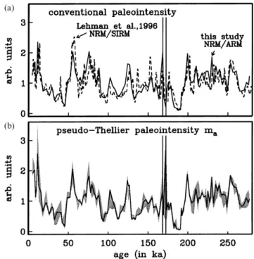
Figure 9. (a) Palaeointensity estimate using a conventional method.
Dashed line is from Lehman et al. (1996), NRM
25mT/SIRM; solid line is from this study, NRM
25mT/ARMmax. ( b) Pseudo-Thellier palaeo-intensity estimate m
a. Solid line is the best-fit slope mathrough at least four successive data points from the NRM left versus ARM gained plot for each sample (Fig. 1b); shaded areas indicate upper and lower limits of 90 per cent confidence level of slope ma determined by jackknife resampling. Peaks in conventional intensity often correspond to maximum values of ma. Both palaeointensity estimates show low-intensity intervals at 40–45 ka and 180–190 ka.
Table 1. Geochemical elements from core SU92–18 with their mean
values and standard deviations. The geometric mean is given when an element is logarithmically distributed.
Lognormal distributions element unit geometric b+s
L b−sL mean, b P ppm 738 951 573 S ppm 1377 1853 1024 Ni ppm 18.2 26.8 12.3 Ba ppm 392 521 296 Ti % 0.40 0.61 0.26 Fe % 2.06 3.02 1.40 Al % 2.95 3.96 2.19 K % 1.12 1.42 0.88 Normal distributions
Element Unit Mean Standard deviation
Figure 8. (a) IRM acquisition and subsequent DC demagnetization
with a back field of sample 759. SIRM is 29.9 A m−1. (b) Henkel plot
Mn ppm 643 125
(Henkel 1964): IRM acquired at given peak field versus IRM left at
Zr ppm 177 65
the same back field. Field steps as in (a). The absence of a linear
Sr ppm 1115 160
relationship could indicate magnetic interaction. (c) Cisowski plot
CaCO
3 % 59.4 9.8
(Cisowski 1981): IRM acquisition and subsequent AF- demagnetization.
Na % 2.4 0.4
IRM
250mTis 28.8 A m−1. The crossing point of 35 per cent, rather than 50 per cent, also indicates magnetic interaction. All intensities are normalized by their maximum values.
anti-correlates withk. This suggests that the magnetic particles in the sediment have a detrital origin. Moreover, the pattern of k calculated on a carbonate-free basis closely resembles that of k. This indicates that the variations in k are not a
Figure 10. Geochemical results compared tok: (a) k (filled symbols) and k on a carbonate-free basis (open symbols) in 10−6 SI; (b) Ti (per cent); (c) CaCO
3(per cent); (d) Mn (ppm); (e) S (ppm). Ti and Ca show good correlations withk, suggesting that magnetic particles are of detrital origin. Maxima in Mn correspond to maxima in Ti, indicating that diagenesis did not affect this sediment to a major extent. S shows a remarkable peak at the low-intensity two-component NRM interval of 636–664 cm depth.
result of dilution by CaCO3. Similar to k, the patterns in suggests that in the top 130 cm transient processes may occur which complicate whole-core analysis. Therefore, in the com-most parameters do not significantly change upon carbonate
correction; only Al and K show a slight decrease in amplitude, bined geochemical/magnetic analysis we have omitted the top 130 cm.
whilst S variations show somewhat increased amplitudes.
Fe and Mn are indicators of palaeoredox conditions (Finney Fuzzy c-means clustering was performed for two to seven clusters. Cluster centres are given in Table 2 for the two-cluster et al. 1988). The Fe pattern corresponds to Ti, which indicates
that Fe is detrital and has not migrated as a result of diagenesis. model and in Table 3 for the seven-cluster model. The most prominent features of the seven-cluster model are summarized Mn (Fig. 10d) shows a background level, with peaks
corre-sponding to peaks in Ti. This also suggests that the effects of in Fig. 11. Bivariate scatter plots of CaCO
3versus Ti (Figs 12a diagenesis on the NRM are not important in this core. S
(Fig. 10e) shows a different behaviour: maxima in S correspond
Table 2. Fuzzy c-means cluster centres for the two-cluster model.
more or less to minima in Ti. The interval of relatively high S
Cluster 1 is mainly detrital, cluster 2 mainly calcareous. CaCO 3, Al,
content corresponds to the two-component low-intensity NRM
Ti and K in per cent, ARM
maxand ARMmax/k in 10−6 Am2, k in 10−6
interval (636–664 cm).
SI, S, Mn, Zr and Ba in ppm, Fe/Al dimensionless.
3.4 Fuzzy c-means cluster analysis
We have applied fuzzy c-means cluster techniques on a number of rock magnetic and geochemical parameters. (1) Rock mag-netic:k and ARMmax as parameters indicative of concentration; ARMmax/k as a grain size indicator; (2) geochemical: Ca and Ba as proxies for biogenic input; Al, Ti and Zr for detrital input; Fe/Al, Ba and Mn as indicators for redox potential; S indicates anoxic conditions and K is a proxy for pore-water content. NRM
25mT and palaeointensity estimates were not included in the cluster analysis because we aimed to assess whether the palaeointensity record would be influenced by non-magnetic parameters. In a preliminary geochemical cluster analysis, the top 130 cm of the core disturbed clustering for the rest of the core. Some samples from the top formed separate clusters with only one or two samples per cluster, while the rest of the samples from the top were intermediate cases. This
Table 3. Fuzzy c-means cluster centres for the seven-cluster model. Units as in Table 2.
Clusters are ranked according to their CaCO3content. Clusters 1, 2 and 3 are detrital; clusters 5, 6 and 7 are calcareous. Cluster 4 is a transitional detrital/calcareous cluster.
Figure 11. Schematic representation of cluster characteristics for the seven-cluster model.
and b) and Zr versus Ti ( both detrital input indicators) cluster, containing more CaCO3, is interpreted as a calcareous cluster with a mainly biogenic origin.
(Figs 12c and d) illustrate the interpretation of the cluster analysis. CaCO
3was calculated from Ca, assuming that 98 per By increasing the number of clusters, a more subtle character within the detrital and calcareous clusters emerges. The detrital cent of Ca resides in CaCO3. For the two-cluster model
(Fig. 12a), one cluster shows a low CaCO
3and high Ti content category is split into a tephra layer (very high Ti content, cluster 1), a detrital cluster with relatively high Ti (cluster 3) and the other cluster a relatively high CaCO
3 and low Ti
content. Intermediate samples fall between the two clusters. and a cluster with relatively a high Zr content (cluster 2). The calcareous category divides into a cluster with a high S content The first cluster, with high Ti, Zr and Al contents, is interpreted
as a cluster with dominant detrital characteristics. The second (cluster 7) and clusters with relatively high ARM
max andk,
Figure 12. Bivariate cluster plots. (a) CaCO3 versus Ti for two clusters: cluster 1=detrital (filled circles), cluster 2=calcareous (open circles),
intermediate samples=crosses. (b) CaCO
3versus Ti for seven clusters: cluster 1=filled triangles; 2=filled circles; 3=filled squares; 4=filled diamonds; 5=open triangles; 6=open circles; 7=open squares; intermediate samples=crosses. Detrital clusters are 1, 2 and 3; calcareous clusters are 5, 6 and 7. Cluster 4 is a transitional detrital/calcareous cluster. See Fig. 11 for cluster characteristics;. (c) Zr versus Ti for two clusters, symbols as in (a). (d) Zr versus Ti for seven clusters, symbols as in ( b). The two lines of clusters—1, 3, 6 and 2, 4, 5—indicate different source areas.
and low Ti within the calcareous category (clusters 6 and 5, Detrital material is readily available and will be transported because of increased erosion. This results in mainly detrital respectively). The interval of low palaeointensity at 180–190 ka
is recognized as (part of ) a separate cluster (cluster 4) which samples, apparently with a relatively high Ti content. As the climate warms up, vegetation reappears and the detrital input has relatively high S.
In the seven-cluster model, two groups of clusters develop decreases, resulting in a relatively higher calcareous content. Also, prevailing wind directions might change because of the apart from the detrital and calcareous division. This is
illustrated Fig. 12(d). One group consists of clusters 1, 3 and 6 shifting of high- and low-pressure systems, and therefore the provenance might change as well.
(filled triangles, filled squares and open circles), the other group
of clusters 2, 4 and 5 (filled circles, filled diamonds and open From the calcareous clusters, it is remarkable that cluster 6 occurs predominantly in warmer climates and cluster 7 in colder triangles). These groups of clusters lie on lines with different
slopes. Moreover, inspection of the correlation matrix of climates. During warmer periods there is increased precipitation and chemical erosion, resulting in increased run-off and a all parameters considered (not shown) reveals that log(Ti)
correlates highly with log(ARMmax), log(Fe), log(Al), log(k) relatively more detrital calcareous cluster (cluster 6) than in colder periods (cluster 7). Cluster 2 (detrital, with highest Zr) and anti-correlates highly with Ca. Z, however, correlates highly
only with log(K), correlates moderately with log(Al) and anti- typically occurs during (minor) changes from warming to cooling and vice versa. Cluster 4 dominates on the cooling parts of correlates moderately with Ca. Thus, the detrital indicators Ti
and Z show clearly different behaviour. Calculation of para- the curve. Although we see a correlation between the clusters and climate we are unable to explain all of the connections. meters on a carbonate-free basis (e.g. Fig. 10a) indicates that
variation in the parameters is not due to dilution by CaCO3. Additional biostratigraphical and oceanographical information is probably needed for a more complete understanding of These observations point to two different source areas of
detrital material: one with relatively high Ti and low Zr and the relations. the other with high Zr and low Ti.
For the seven-cluster model, the cluster assignment of each
4 D I S C U S S I O N sample is plotted on the d18O-SPECMAP curve (Fig. 13).
Cluster 3 samples (detrital and highk, Ti, Al, Ba) occur during
4.1 Spectral analysis and correlation with climate periods of rapid warming of the climate. We associate this
kind of detrital sample with increased detrital input after the Changes in ice-sheet volume caused by orbital forcing are recorded in shells of for example planktonic foraminifera as end of an ice age. During rapid warming (i.e. melting of the
ice cover) there is still no or little vegetation in source areas. fluctuations in the d18O ratio. We test for potential climate
Figure 13. Seven-cluster model andd18O-SPECMAP (Imbrie et al. 1984). Symbols as in Fig. 12(b). Cluster 3 samples (filled squares) predominantly occur during rapid warming. Cluster 6 samples (open circles) occur during warmer climates, cluster 7 samples (open squares) during colder climates. Note that the upper 130 cm of the core was not included in the fuzzy c-means cluster analysis.
influence on the magnetic parameters and palaeointensity advantage of performing the pseudo-Thellier method. Unlike the conventional method, the pseudo-Thellier method used in estimates of the present study by performing a spectral analysis.
The spectral analysis was performed with the algorithm combination with a jackknife procedure provides an error estimate. Intensity information contained in the NRM signal of Roberts et al. (1987), which was developed for unequally
spaced time-series. In this procedure, the ‘dirty’ spectra are of a whole range of (relatively higher) coercivities is included in the palaeointensity estimate, not just one single point as first calculated and then ‘ed’ by iteration. The procedure
has been repeated for different window steps, gains and with the conventional method.
In the conventional ARM normalizing method, saturation numbers of iterations. The parameters which gave the
most consistent spectra (dF=1, gain=1, 500 iterations) were of ARM is generally not tested. A standard alternating peak field is applied to each sample. This peak field might saturate chosen for all magnetic and geochemical parameters.
Frequency spectra of the parameters are checked for the different samples to a different degree, introducing an artefact in the normalization parameter. In the pseudo-Thellier method presence of the Earth’s orbital frequencies. All spectra are
normalized by their mean values. Thed18O record of SU92–18 ARM saturation is not required because a number of ARM acquisition steps are used in the determination of the palaeo-contains the Earth’s orbital periods of eccentricity (100 kyr),
obliquity (41 kyr) and climatic precession (23 kyr) (Fig. 14a). intensity. Although not required, stepwise ARM acquisition of the pseudo-Thellier method provides a check of ARM Also, the spectra of magnetic parameters k and NRM show
frequencies that can be attributed to obliquity (41 kyr) and saturation.
However, there are some pitfalls with the pseudo-Thellier precession (23 and 19 kyr) (Fig. 14b). The ARM spectrum
(not shown) is identical to that ofk. The spectrum of the NRM palaeointensity record which appear for the conventional palaeointensity method as well. Problems arise for multi-normalized by ARM in the conventional way (Fig. 14c) still
shows spectral amplitudes at the climatic frequencies, particu- component NRMs. With multicomponent NRMs the slope m a cannot be determined reliably because the intensity of the larly at 23 kyr−1. This is also true for the pseudo-Thellier
palaeointensity estimate ma. Thus, normalizing the NRM has primary component is obscured by secondary components. On the other hand, the stepwise NRM demagnetization required not removed all environmental influences.
As with the magnetic parameters, the geochemical para- for the pseudo-Thellier method reveals a multicomponent NRM if present.
meters are also influenced by climate. Ba (not shown) and Ca, both regarded as palaeoproductivity indicators (e.g. Elderfield 1990) consistently show power at all climatic frequencies
4.3 Magnetic-grain-size estimates (Fig. 14d). Al (not shown) and Ti, representing detrital input,
show peaks at obliquity and precession frequencies. S, however, The ratio ARM/k is generally regarded as a grain-size indicator. For magnetite, this ratio varies inversely with grain size (King seems to be influenced by obliquity and precession (19 kyr).
For Ca and Ti the 19 kyr precession peak seems to be shifted et al. 1982). However, ARM and k respond differently to changes in grain size. Therefore, this interpretation might not to a shorter period (approximately 17 kyr).
be so straightforward. ARM/k is not only sensitive to the average grain size of the magnetic particles, but also to the 4.2 Comments on the pseudo-Thellier method
grain-size distribution. A relatively broader distribution with the same average particle size suffers from two effects: higher Although palaeointensity records obtained by the
con-ventional method and the pseudo-Thellier method do not ARM, because of relatively more SD particles, and higherk from relatively more MD particles. The resulting effect on the differ considerably for this core, there is still an important
A third effect which must be considered is the clay-mineral content. This deserves special attention whenk is low and is not mainly determined by ferrimagnetic minerals. For example, chlorite has a k value considerably higher than kaolinite. Which clay minerals dominate depends on the type of weather-ing and hence on climate (e.g. Chamley 1989). The ARM/k ratio might thus be biased by varying contributions from different clay minerals. In the present case, however, ARM and k are perfectly correlated (r=0.985), so we can assume that the main part of k is residing in ferrimagnetic material and that there is no significant paramagnetic contribution from clay minerals.
4.4 Reversal excursions and palaeointensities
The palaeointensity record and the NRM directional record (Figs 9 and 5) indicate that the sediments from this core have recorded the Laschamps excursion. The Blake excursion, how-ever, has not been recorded even though the Blake is globally recognized (see the compilation of Nowaczyk et al. 1994). The non-recording of the Blake could mean either that the Blake has not occurred globally or that the sediment is not always a good recorder, at least not of directions. Neither chemical nor rock magnetic parameters indicate that this excursion was erased by diagenesis.
The low-intensity interval from 180 to 190 ka shows a ‘soft’ component with coercivities up to 80–100 mT. The hard component (>100 mT) clearly has a different direction from the soft component. The directions of the hard component match the directions of the remainder of the record, while the ‘soft’ component significantly deviates (declination−120° and shallow/negative inclination). The results could indicate that the hard components correctly recorded the magnetic signal during or shortly after deposition and the ‘soft’ components are overprints. However, coercivities are too high to be con-sidered as viscous. Alternatively, the observed NRM behaviour of this interval could be an artefact of the AF demagnetization process, because the hard component does not have a stable endpoint. The most likely interpretation is that the ‘soft’ components show the true directions, with the hard com-ponents acquired later by the geomagnetic field existing then, for example through later low-temperature oxidation. The timing of this excursion coincides with the Icelandic Basin reversal excursion at 188 ka (Channell et al. 1997). A distinct intensity low at 180–190 ka is also reported in the SINT-200 stack of Guyodo & Valet (1996) and in an independent 10Be-stack (Frank et al. 1997). It is remarkable that this
two-(a)
(b)
(c)
(d)
component NRM interval contains high S values relative to
Figure 14. Spectral analysis performed with the algorithm of
the rest of the record. However, thermomagnetic analysis did
Roberts et al. (1987). Milankovitch periods, indicated by dashed
not show magnetic sulphides in this interval. We do not have
vertical lines, are 100 kyr for eccentricity, 41 kyr for obliquity and 23
an explanation for the coincidence of the high S content and
and 19 kyr for climatic precession. (a) Dirty and clean frequency
the low-intensity two-component NRM in this interval.
spectrum ofd18O of SU92–18; (b) clean frequency spectra of magnetic parameters NRM
25mTand k; (c) clean frequency spectra of pseudo- In their high-sedimentation-rate palaeointensity record Thellier palaeointensity estimate m
aand conventional palaeointensity from ODP Site 983 in the Iceland Basin, Channell et al. (1997) estimate NRM25mT/ARMmax; (d) clean spectra of Ti, S and Ca. All tied successive palaeointensity features (H: high; L: low) to spectra are normalized by their mean values. the correlative oxygen isotope stages. Some features can be
recognized in the Azores record, e.g. 3–2 L (~40 ka), 5–3 L (~95 ka), 8–1H (~250 ka), while others seem to show an ratio ARM/k is unknown. Moreover, ARM and k do behave
differently with concentration variations. Even at low concen- offset in age of approximately 5 kyr. This may be explained by small uncertainties in the respective age models. There are trations, magnetic interaction influences ARM, so the ratio
ARM/k is affected by concentration as well (Yamazaki & Ioka several features, however, which are contradictory, for example their intensity low 5–5 L at approximately 125 ka compares 1997; Sugiura 1979).
unfavourably with the high intensity in our record at that age, and Lisa Tauxe for their useful discussions and Cor de Boer for his help with the Curie balance measurements and inter-and the interval 200–250 ka also shows discrepancies. In this
interval, Channell et al. (1997) attribute the intensity low 7–4 L pretation. The critical and constructive comments of an anonymous reviewer greatly improved this manuscript This to the Pringle Falls excursion (Herrero-Bervera et al. 1994)—
which is equivalent to the Jamaica event of Ryan (1972), study is partly supported by the Netherlands Geoscience Foundation (GOA/NWO). This work was conducted under redated at approximately 210 ka (Langereis et al. 1997)—
whereas we find no evidence for a clear intensity minimum; the programme of the Vening Meinesz research School of Geodynamics. A table with all relevant data can be found at neither record shows excursional directions. Finally, in the
Iceland Basin there is evidence for another excursion, in both the URL www.geo.uu.nl/geophysics/html/paleo/forth.html. direction (declinations) and intensity (intensity low 8–2 L) at
approximately 263 ka, which correlates well with the Calabrian
Ridge 0 (CR0) reversal excursion from the Mediterranean at R E F E R E N C E S 261±3 ka (Langereis et al. 1997); in the Azores record we
Banerjee, S.K. & Mellema, J.P., 1974. A new method for the
deter-find a corresponding intensity low, but no directional evidence
mination of paleointensity from the A.R.M. properties of rocks,
for this excursion.
Earth planet. Sci. L ett., 23, 177–184.
Bard, E., Hamelin, B., Fairbanks, R.G. & Zindler, A., 1990. Calibration of the14C timescale over the past 30,000 years using mass
spectro-4.5 Palaeointensity m
aand the seven-cluster model metric U-Th ages from Barbados corals, Nature, 345, 405–410. From the spectral analysis (Fig. 14c) it is clear that the palaeo- Bezdek, C.J., 1981. Pattern Recognition with Fuzzy Objective Function intensity estimate ma is not free from climatic influences. The Algorithms, Plenum Press, New York.
question arises why we still see climate in the palaeointensity Chamley, H., 1989. Clay Sedimentology, Springer-Verlag, New York. Channell, J.E.T., Hodell, D.A. & Lehman, B., 1997. Relative
paleo-record. An attempt to answer this question is made with the
intensity andd18O at ODP Site 983 (Gradar Drift, North Atlantic)
combined rock magnetic/geochemical fuzzy c-means cluster
since 350 ka, Earth planet. Sci. L ett., 153, 103–118.
analysis. This independent method shows climatic influence on
Cisowski, S., 1981. Interacting vs. non-interacting single domain
the properties of the core as well. However, we do not see a
behavior in natural and synthetic samples, Phys. Earth planet. Inter.,
clear relationship between the palaeointensity ma and the 26, 56–62.
seven-cluster model. The clusters are not related to particular de Boer, C.B. & Dekkers, M.J., 1996. Grain-size dependence of the intervals of ma values like in the d18O record (Fig. 13), except rock magnetic properties for a natural maghemite, Geophys. Res.
cluster 4 with high S and low palaeointensity. We have to keep L ett., 23, 2815–2818.
in mind, however, that this low appears in the two-component Dekkers, M.J., Langereis, C.G., Vriend, S.P., van Santvoort, P.J.M. &
NRM interval, so palaeointensities could not be determined Lange, G.J., 1994. Fuzzy c-means cluster analysis of early diagenetic effects on natural remanent magnetisation acquisition in a 1.1 Myr
reliably.
piston core from the Central Mediterranean, Phys. Earth planet. Inter., 85, 155–171.
5 C O N C L U S I O N S Efron, B., 1982. T he Jackknife, the Bootstrap and Other Resampling
Plans., Society for Industrial and Applied Mathematics, Philadelphia,
The palaeointensity records show two distinct lows at 40–45 ka
PA.
and 180–190 ka. The former corresponds to the Laschamps Elderfield, H., 1990. Tracers of ocean paleoproductivity and paleo-excursion; the latter represents the Icelandic Basin excursion. chemistry: an introduction, Paleoceanography, 5, 711–717. The Blake, Jamaica/Pringle Falls and Calabrian Ridge 0 (CR0) Fearon, M., Chantrell, R.W. & Wohlfarth, E.P., 1990. A theoretical excursions are not recorded in these sediments, although study of interaction effects on the remanence curves of particulate
relatively low-intensity intervals are found at~115 ka (Blake?) dispersions, J. Mag. Magnetic Mater., 86, 197–206.
Finney, B.P., Lyle, M.W. & Heath, G.R., 1988. Sedimentation at
and~265 ka (CR0?).
MANOP site H (eastern equatorial Pacific) over the past 4000,000
The conventional and pseudo-Thellier methods for
palaeo-years: climatically induced redox variations and their effects on
intensities give similar results. Both records are contaminated
transition metal cycling, Paleoceanography, 3, 169–189.
by climate, as indicated by spectral analysis. However, the
Frank, M., Schwarz, B., Baumann, S., Kubik, P.W., Suter, M. &
extent of the climate influence is difficult to quantify. The fuzzy
Mangini, A., 1997. A 200 kyr record of cosmogenic radionuclide
c-means clustering analysis resulted in a model with mainly
production rate and geomagnetic field intensity from10Be in globally
calcareous versus mainly detrital clusters. Samples from detrital stacked deep-sea sediments, Earth planet. Sci. L ett., 149, 121–129. clusters predominantly appear during rapid warming up, after Guyodo, Y. & Valet, J.-P., 1996. Relative variations in geomagnetic the end of an ice age. The initial lack of vegetation provides intensity from sedimentary records: the past 200,000 years, Earth
an increased detrital input; when vegetation starts to develop, planet. Sci. L ett., 143, 23–36.
Hartl, P. & Tauxe, L., 1996. A precursor to the Matuyama/Brunhes
the sediment input becomes more calcareous. Although both
transition-field instability as recorded in pelagic sediments, Earth
the pseudo-Thellier palaeointensity m
a and fuzzy cluster planet. Sci. L ett., 138, 121–135. analysis on rock magnetic and geochemical data show climatic
Henkel, O., 1964. Remanenzverhalten und Wechselwirkungen in
influences, we have not been able to find a viable connection
hartmagnetischen Teilchenkollektiven, Phys. Stat. Sol., 7, 919–929.
between the clusters and m
a. Herrero-Bervera, E. et al., 1994. Age and correlation of a paleomagnetic episode in the western United States by 40Ar/39Ar dating and tephrochronology: The Jamaica, Blake, or a new polarity episode?,
A C K N O WL E D G M E N T S
J. geophys. Res., 99, 24 091–24 103.
Thanks are due to Laurent Labeyrie for access to core Housden, J. & O’Reilly, W., 1990. On the intensity and stability of the SU92–18. Benoıˆt Lehman is thanked for his help with sampling natural remanent magnetization of ocean floor basalts, Phys. Earth
planet. Inter., 64, 261–278.
the core and access to his data. We acknowledge Frits Hilgen
Imbrie, J. et al., 1984. The orbital theory of Pleistocene climate: Raisbeck, G.M., Yiou, F., Bourles, D., Lorius, C., Jouzel, J. & Barkov, N.I., 1987. Evidence for two intervals of enhanced 10Be support from a revised chronology of the marined18O record, in
Milankovitch and Climate, part 1, ed. Berger, A.L., Imbrie, J., Hays, J., deposition in Antarctic ice during the last glacial period, Nature,
326, 273–277.
Kukla, G. & Saltzman, B., pp. 269–305, D. Reidel, Dordrecht.
Kaufman, L. & Rousseeuw, P.J., 1990. Finding Groups in Data: an Roberts, D.H., Leha´r, J. & Dreher, J.W., 1987. Time series analysis with clean. I. derivation of a spectrum, Astr. J., 93, 968–989. Introduction to Cluster Analysis, John Wiley, New York.
King, J.W., Banerjee, S.K., Marvin, J. & O¨ zdemir, O., 1982. A Robinson, C., Raisbeck, G.M., Yiou, F., Lehman, B. & Laj, C., 1995. The relationship between10Be and the geomagnetic field strength comparison of different magnetic methods for determining the
relative grain size of magnetite in natural minerals, some results for records in central North Atlantic sediments during the last 80 ka, Earth planet. Sci. L ett., 136, 551–557.
lake sediments, Earth planet. Sci. L ett., 59, 404–419.
Kok, Y.S., Tauxe, L. & Pick, T., 1998. Jackknife resampling for Ryan, W.B.F., 1972. Stratigraphy of late Quaternary sediments in the Eastern Mediterranean, in T he Mediterranean Sea: A Natural paleointensities of the Earth’s magnetic field, Geophys. Res. L ett.,
submitted. Sedimentation L aboratory, pp. 149–169, ed. Stanley, D.J., Dowden, Hutchinson & Ross, Stroudsberg, PA.
Langereis, C.G., de Dekkers, M.J., Lange, G.J., Paterne, M. & van
Santvoort, P.J.M., 1997. Magnetostratigraphic and astronomical Schwartz, M., Lund, S.P. & Johnson, T.C., 1996. Environmental factors as complicating influences in the recovery of the quantitative calibration of the last 1.1 Myr from an eastern Mediterranean piston
core and dating of short events in the Brunhes, Geophys. J. Int., geomagnetic-field paleointensity estimates from sediments, Geophys. Res. L ett., 23, 2693–2696.
129, 75–94.
Lehman, B., Laj, C., Kissel, C., Mazaud, A., Paterne, M. & Labeyrie, L., Sugiura, N., 1979. ARM, TRM and magnetic interactions: concen-tration dependence, Earth planet. Sci. L ett., 42, 451–455.
1996. Relative changes of the geomagnetic field intensity during the
last 280 kyear from piston cores in the Ac¸ores area, Phys. Earth Tauxe, L., 1993. Sedimentary records of relative paleointensity of the geomagnetic field: theory and practice, Rev. Geophys., 31, planet. Inter., 93, 269–284.
Lowrie, W., 1990. Identification of ferromagnetic minerals in a rock 319–354.
Tauxe, L., Pick, T. & Kok, Y.S., 1995. Relative paleointensity in by coercivity and unblocking temperature properties, Geophys. Res.
L ett., 17, 159–162. sediments: a pseudo-Thellier approach, Geophys. Res. L ett., 22, 2885–2888.
Martinson, D.G., Pisias, N.G., Hays, J.D., Imbrie, J., Moore, T.C. &
Shackleton, N.J., 1987. Age dating and the orbital theory of the ice Valet, J.-P. & Meynadier, L., 1993. Geomagnetic field intensity and reversals during the past four million years, Nature, 366, ages: development of a high resolution 0–300 000 years stratigraphy,
Quat. Res., 27, 1–29. 234–238.
Valet, J.-P. & Meynadier, L., 1998. A comparison of different Mazaud, A., Laj, C., Bard, E., Arnold, M. & Tric, E., 1991. Geomagnetic
field control of14C production over the last 80 ky: implications for techniques for relative paleointensity, Geophys. Res. L ett., 25, 89–92.
the radiocarbon time-scale, Geophys. Res. L ett., 18, 1885–1888.
McFadden, P.L. & McElhinny, M.W., 1988. The combined analysis of van Velzen, A.J. & Zijderveld, J.D.A., 1995. Effects of weathering on single-domain magnetite in Early Pliocene marine marls, Geophys. remagnetization circles and direct observations in palaeomagnetism,
Earth planet. Sci. L ett., 87, 161–172. J. Int., 121, 267–278.
Weeks, R.J., Laj, C., Endignoux, L., Mazaud, A., Labeyrie, L., Meynadier, L., Valet, J.-P., Weeks, R., Shackleton, N.J. & Hagee, V.L.,
1992. Relative geomagnetic intensity of the field during the last Roberts, A.P., Kissel, C. & Blanchard, E., 1995. Normalised natural remanent magnetisation intensity during the last 240 000 years from 140 ka, Earth planet. Sci. L ett., 114, 39–57.
Mullender, T.A.T., van Velzen, A.J. & Dekkers, M.J., 1993. Continuous piston cores from the central North Atlantic Ocean: geomagnetic field intensity or environmental signal?, Phys. Earth planet. Inter., drift correction and separate identification of ferrimagnetic and
paramagnetic contributions in thermomagnetic runs, Geophys. J. Int., 87, 213–229.
Wohlfarth, E.P., 1958. Relations between different modes of acquisition
114, 663–672.
Nowaczyk, N.R., Frederichs, T.W., Eisenhauer, A. & Gard, G., 1994. of the remanent magnetization of ferromagnetic particles, J. appl. Phys., 29, 595–596.
Magnetostratigraphic data from late Quaternary sediments from
the Yermak Plateau, Arctic Ocean: evidence for four geomagnetic Yamazaki, T. & Ioka, N., 1997. Cautionary note on magnetic grain-size estimation using the ratio of ARM to susceptibility, Geophys. polarity events within the last 170 Ka of the Brunhes Chron,
Geophys. J. Int., 117, 453–471. Res. L ett., 24, 751–754.