Estimation of the CO2 and CH4 fluxes in France using atmospheric concentrations from ICOS network and data-assimilation techniques

HAL Id: tel-01914926

https://tel.archives-ouvertes.fr/tel-01914926

HAL is a multi-disciplinary open access

archive for the deposit and dissemination of sci-entific research documents, whether they are pub-lished or not. The documents may come from teaching and research institutions in France or

L’archive ouverte pluridisciplinaire HAL, est destinée au dépôt et à la diffusion de documents scientifiques de niveau recherche, publiés ou non, émanant des établissements d’enseignement et de recherche français ou étrangers, des laboratoires

Estimation of the CO2 and CH4 fluxes in France using

atmospheric concentrations from ICOS network and

data-assimilation techniques

Abdelhadi El Yazidi

To cite this version:

Abdelhadi El Yazidi. Estimation of the CO2 and CH4 fluxes in France using atmospheric concen-trations from ICOS network and data-assimilation techniques. Meteorology. Université Paris Saclay (COmUE), 2018. English. �NNT : 2018SACLV067�. �tel-01914926�

Estimation of the CO

₂

and CH

₄

fluxes in France using atmospheric

concentrations from ICOS network

and data-assimilation techniques.

Thèse de doctorat de l'Université Paris-Saclay

préparée à Université de Versailles Saint-Quentin-en-Yvelines

École doctorale n°129 Sciences de l’environnement Ile de France

(SEIF)

l'Environnement

Thèse soutenue au LSCE, le 1er octobre 2018, par

Abdelhadi El Yazidi

Composition du Jury : M. Philippe Bousquet

Professeur, LSCE Président M. Christoph Gerbig

Chargé de recherche, MPBI Rapporteur Mme. Greet Janssen-Maenhout

Chargé de recherche, JRC Rapporteur Mme. Christine Lac

Chargé de recherche, CRNM Examinateur M. Vincent-Henri Peuch

Chargé de recherche, ECMWF Examinateur M. Philippe Ciais

Directeur de recherche, LSCE Directeur de thèse M. Michel Ramonet

Chargé de recherche, LSCE Co-Directeur de thèse

NNT : 2018SACLV067

Titre :Estimation des flux de CO

et de CH

en France en utilisant les concentrations

atmosphérique du réseau ICOS et les techniques d'assimilation de données

Mots clés : Gaz à effet de serre, CO

, CH

, France, inversion

Depuis la révolution industrielle, les croissances économique et démographique ont augmenté de manière exponentielle induisant la hausse de la combustion d’énergies fossiles, telles que le charbon, le pétrole, et le gaz naturel. La combustion de ces sources d’énergie conduit à l’émission de gaz à effet de serre (GES), principalement le dioxyde de carbone (CO2) et le méthane (CH4), qui par leur accumulation dans l’atmosphère entraînent une accentuation de l’effet de serre.

Selon le GIEC (Groupe d'experts Intergouvernemental sur l'Évolution du Climat), l’implication des émissions anthropiques dans l’augmentation de l’effet de serre est extrêmement probable avec un pourcentage de certitude qui dépasse 95%. Toutefois, l’estimation des bilans régionaux d'émissions de GES reste très incertaine. L’objectif de cette thèse est de contribuer à l’amélioration des estimations des bilans régionaux de GES en France, en utilisant les techniques de la modélisation inverse et les mesures atmosphériques du CO2 et de CH4 fournis par le réseau ICOS (Integrated Carbon Observation System). Dans un premier temps, on s’est focalisé sur l’étude des concentrations mesurées de CO2, CH4 et CO (monoxyde de carbone). Cette étude a pour objectif, l'identification des mesures atmosphériques contaminées par les émissions locales (quelques kilomètres au tour de la station) et qui provoque ce qu’on appelle « les pics de concentrations ». Trois méthodes ont été appliquées sur des séries temporelles fournies par quatre stations du réseau ICOS, afin de déterminer leur degré de contamination. Ainsi, les résultats des différentes méthodes ont été comparés à un inventaire de données contaminées fourni par les gestionnaires des stations. À l’issue de ce travail, une méthode a été proposée pour effectuer un nettoyage automatique des séries de mesure du réseau ICOS.

Dans un deuxième temps, le modèle régional de chimie-transport CHIMERE est utilisé pour simuler les concentrations atmosphériques du CO2 et du CH4 de l’année 2014 sur un domaine centré sur la France. L’objet de cette étude est d’évaluer la sensibilité des concentrations simulées en utilisant différentes données d’entrées (sensibilité aux transports météorologiques et sensibilité aux flux de surface). Cette analyse a permis de quantifier à la fois les erreurs liées aux transports et les erreurs liées aux flux de surface. Ainsi, la meilleure combinaison des données d’entrée a été sélectionnée pour l’étape d’inversion des flux.

Dans un dernier plan, les mesures atmosphériques des concentrations de CO2 et du CH4 sont utilisées par le système d’inversion PYMAI (Berchet et coll., 2013 et 2015) afin d’estimer les bilans régionaux d'émission de CO2 et CH4 en France. L’inversion est réalisée pour un mois d’hiver (janvier) et un mois d’été (juillet) en utilisant le modèle de transport CHIMERE. Le résultat de ce travail a permis la quantification les émissions de CO2 et de CH4 à l'échelle nationale et régionale, ainsi qu’une réduction d’incertitude bilans nationaux à hauteur de 35 %.

Title : Estimation of the CO

and CH

, fluxes in France using atmospheric concentrations

from ICOS network and data-assimilation techniques

Keywords : Greenhouse gas, CO

, CH

, France, inversion

Since the industrial revolution, the economic and the demographic growths have increased exponentially, leading to an enhancement of the fossil fuels combustion, such as coal, oil, and natural gas. Consuming these source of energy amplifies the greenhouse gas emissions, mainly carbon dioxide (CO2) and methane (CH4), whose accumulation in the atmosphere lead to the increase of the greenhouse effect. According to the 5th assessment report of the Intergovernmental Panel on Climate Change (IPCC), it is extremely likely (95-100% of certainty) that the observed increase in the greenhouse effect is related to the increase of the anthropogenic emissions. However, the estimations of the GHG budget at the regional and the national scales remains highly uncertain. The aim of this thesis is to improve the estimation of the CO2 and CH4 fluxes in France, using data assimilation techniques and atmospheric measurements provided by the Integrated Carbon Observation System (ICOS) network.

The first phase focuses on analyzing the measured CO2, CH4, and CO (Carbon monoxide) atmospheric concentrations provided by surface monitoring stations. This study is concerned with the problem of identifying atmospheric data influenced by local emissions that can result in spikes in the GHG time series. Three methods are implemented on continuous measurements of four contrasted atmospheric sites. The aim of this analysis is to evaluate the performance of the used methods for the correctly detect the contaminated data. This work allows us to select the most reliable method that was proposed to perform daily spike detection in the ICOS Atmospheric Thematic Centre Quality Control (ATC-QC) software.

Secondly, we simulate the atmospheric concentrations of CO2 and CH4 using the chemistry transport model CHIMERE in a domain centered over France for the year 2014. The objective of this study is to evaluate the sensitivity of simulated concentrations using different input data (sensitivity to the meteorological transport and sensitivity to the surface fluxes). This work led to the quantification of both the transport and surface fluxes errors based on the combination of different simulations. Thus, the most reliable combination of the best input data was selected for the flux inversion study.

Lastly, the measured CO2 and CH4 concentrations are used by the PYMAI inversion system (Berchet et al., 2013 and 2015) in order to estimate the CO2 and CH4 fluxes in France. The Inversion is performed for one month in winter (January) and one month in summer (July), using the transport model CHIMERE. The inversion results have provided very interesting results for the regional estimation of the CO2 and CH4 surface fluxes in France with an uncertainty reduction that may attain 35% of the national totals.

Acknowledgments

First of all, I would like to express my special appreciation and gratitude to Philippe Ciais, Michel Ramonet, Isabelle Pison and Grégoire Broquet for supervising my Ph.D. You have been a tremendous mentors for me. Thank you, Philippe, for encouraging my research and guiding my scientific learning. Philippe, your advice has inspired and helped me to grow as a research scientist. Thank you, Michel, for your endless support and the time you spent helping me with this thesis. Michel, the joy and the enthusiasm you have for science were catching and motivational for me, even during hard times. Thank you, Isabelle and Grégoire, for your advice, for having pursued my thesis, and for all the time you spent explaining re-explaining me some concepts that were abstract to me.

I would like to thank Christoph Gerbig and Greet Maenhoult for their acceptance to review this thesis. Christine Lac and Vincent-Henri Peuch, thank you for accepting the be part of my Ph.D. jury. I would like to thank also Dominik Brunner and Martina Schmidt for the inspiring discussions and for the time they spent during the thesis committee meeting. Your advice and constructive remarks allowed me to advance the Ph.D. works.

I would like to thank the Climate-Kic for financing this thesis. I am also grateful to CEA for all the financial support and the traveling grants provided for the participation in different summer schools and conferences.

I am also grateful to all of the ICOS team members at LSCE for supporting me and being with me during the past three years. Special thanks in particular to the persons in charge of the monitoring programs and to all the people working for maintenance and data quality control of the stations. LSCE administration would not be that efficient without Catherine Huguen and Elsa Cortijo. Thanks to them for their continuous support in administrative procedures.

My special thanks to Antoine Berchet who helped me to get familiar with the PYMAI inversion system. Thank you, Antoine, for being patient with my questions. My warm thanks to my best friends Ettouhami El Yazidi, Mohamed Bouzidi and Tareq Soubai, thank you for all the good and the bad times we spent together, thank you for your endless support and encouragement during the whole Ph.D. Also many thanks to my family, friends, and everyone I met at LSCE: Oussama Rahimi, Amina, Khadija, Radouane, Amouna, Sabina, Ayché, Sébastien, Sarah, Luis, Céline, Julie, Xin, Lamia, Hamza, …

Lastly, and more importantly, A very warm thanks to my parents. Words can not express how grateful I am to my beloved mother Bouchra Naciri and my dearest father Abdelmajid El Yazidi. Thank you for pushing me towards my goals. Thank you for always being there for me and always welcoming me with open arms.

Contents

...2

Chapter I: Introduction...19

I.1Global radiative balance:...19

I.2Role of the greenhouse gases in global warming...20

I.3Carbon budget...22

I.3.1Carbon dioxide cycle...22

I.3.2Methane cycle...24

I.4CO

and CH

atmospheric measurerments...25

I.5Flux estimation approaches :...27

I.5.1Bottom-up approach:...27

I.5.2Top-down approach...28

I.6Estimation of the regional fluxes...29

I.6.1Some techniques for flux optimization...29

I.6.2Estimation of CO

fluxes...30

I.6.1Estimation of CH

fluxes...32

I.7Objective and structure of this thesis...33

Chapter II: Identification of spikes associated with local sources in continuous time series of

atmospheric CO, CO

and CH

...36

II.1Summary...36

II.1.1Context of the study...36

II.1.2Material and methods...37

II.1.3Selection and the optimization of the spike detection methods...37

II.1.4Principal results...38

II.1.5Conclusions and implications...39

II.2Introduction...40

II.3Methodology...43

II.3.1Measurement sites and methods...43

II.3.1.1Measurement sites...43

II.3.1.2Measurement methods...44

II.3.2Spike detection algorithms...45

II.3.2.1Coefficient of variation (COV) method...46

II.3.2.2Standard deviation of the background (SD)...46

II.3.2.3Robust extraction of baseline signal (REBS)...47

II.4Results...49

II.4.1Optimization of the SD and REBS methods...49

II.4.1.1Sensitivity to the parameters of the SD method...49

II.4.1.2Sensitivity to the parameters of the REBS method...51

II.4.2Statistics of the three spike detection methods...53

II.4.1Comparison of SD and REBS methods to detect CH

spikes at the PDM clean-air

mountain station...54

II.4.2Comparison between automatic and manual spike detection...60

III.2.1CHIMERE atmospheric transport model...70

III.2.2Meteorological fields...72

III.2.2.1AROME...73

III.2.2.2ECMWF...73

III.2.1CO

and CH

surface fluxes...73

III.2.1.1Anthropogenic emissions...74

III.2.1.2Vegetation – atmosphere CO2 fluxes...79

III.2.2Atmospheric concentration measurements...80

III.2.3Ecosystem measurements...83

III.3results...84

III.3.1Comparison of the national totals and temporal distribution of IER and EDGAR

anthropogenic fluxes...84

III.3.2Spatial differences between IER and EDGAR totals...85

III.3.3Temporal differences between IER and EDGAR...87

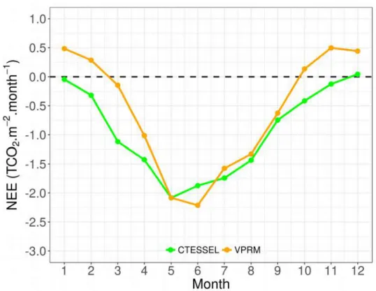
III.3.4Comparison of the biogenic CO

fluxes between CTESSEL and VPRM...90

III.3.4.1Spatial distribution of the modeled fluxes for January and July...91

III.3.4.2Comparison between the modeled and the simulated NEE...93

III.3.5Sensitivity of the concentrations to the meteorological forcing...98

III.3.6Spatial distribution of the AROME/ECMWF differences...109

III.3.7Sensitivity of the concentrations to the surface fluxes...112

III.3.8Spatial distribution of the surface flux differences...122

III.4Conclusions...126

Chapter IV: The potential of a European network for the optimization the CO

and the CH

surface

fluxes in France...129

IV.1Introduction...129

IV.2Methods...131

IV.2.1Inverse problem formalism...131

IV.2.1.1Inversion formalism...131

IV.2.1.2Inverse problem constraints...132

IV.2.1.3Regularization of the inverse problem...132

IV.2.2The solution of the inverse problem:...133

IV.2.3The inversion setup:...134

IV.2.3.1Estimation of the observations and prior variance-covariance matrices...134

IV.2.4The definition of the inverse problem...139

IV.2.4.1Control vector...139

IV.2.4.2Observation vector...141

IV.2.4.3Surface fluxes...143

IV.2.4.4Observation operator...143

IV.3Results...145

IV.3.1Inversion of the CH

fluxes...145

IV.3.1.1Weight of the CH4 atmospheric observations in the inversion...145

IV.3.1.2Comparison of observation and prior flux errors with independent empirical estimates...149

IV.3.1.3Fit of posterior concentrations to observations...153

IV.3.1.4Emission regions constrained by the inversion...156

IV.3.1.5Spatial correlation of the flux errors...159

IV.3.1.6The spatio-temporal scales resolved by the inversion...162

IV.3.1.7Optimized fluxes...165

IV.3.2Inversion of the CO

fluxes...170

IV.3.2.1Weight of the CO2 atmospheric observations in the inversion...170

IV.3.2.2Investigation of the observation and the prior flux errors...172

IV.3.2.4Flux regions constrained by the inversion...180

IV.3.2.5Spatial correlation of the anthropogenic and biogenic flux errors...184

IV.3.2.6The spatio-temporal scales resolved by the inversion...187

IV.3.2.7Optimized fluxes...192

IV.4Conclusions...200

Chapter V: Conclusions and perspectives :...203

V.1Conclusion...203

V.1.1Spike detection algorithms...204

V.1.2Evaluation of the simulated CO

and CH

concentrations...204

V.1.3Estimation of the CO

and CH

fluxes in France...206

V.2Perspectives...208

V.2.1Identification of the local contamination sources...208

V.2.2Atmospheric modeling...209

V.2.3Inverse modeling...210

Chapter VI: References...212

VI.1Appendix...225

VI.1.1Chapter II...225

VI.1.2Chapter III...234

Figures

Figure I.1 : Global radiative balance in the current climate. The numbers in bold correspond to the

estimate of each energy flux in W.m-2 (5th Assessment Report of the Intergovernmental Panel on

Climate Change 2013)...20

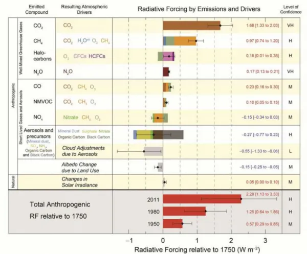
Figure I.2: Radiative forcing of the main anthropogenic (greenhouse gases, aerosol, short-lived gas)

and natural (solar radiation) factors impacting the climate in 2011 compared to 1750 (5th

Assessment Report of the IPCC 2013)...21

Figure I.3: Representation of the carbon cycle. The annual fluxes are estimated in PgC/year and

averaged over the period 2000-2009. The amount of CO2 stored in the three reservoirs is expressed

in PgC. The figure is taken from the 5th assessment report of the intergovernmental panel for the

Climate Change (IPCC 2013)...23

Figure I.4: Representation of the methane cycle. The annual fluxes are estimated in TgCH 4/year

and averaged over the period 2000-2009. The amount of CH4 stored in the three reservoirs is

expressed in TgCH4 . This figure is taken from the 5th assessment report of the intergovernmental

panel for the Climate Change (IPCC 2013)...25

Figure I.5: maps of the GLOBALVIEW, ICOS and RAMCES atmospheric station networks...27

Figure I.6: Panel (A) displays the regions on which the estimated fluxes are aggregated. Panel (B)

represents the estimated net carbon flux and the corresponding uncertainties for the sub-continental

European regions presented in panel (A). The inversion was performed using five atmospheric

transport models as described in Rivier et al., (2010). The figure is taken from Rivier et al., (2010).

...31

Figure I.7: Annual biogenic CO2 budget (GtC/yr) in Europe retrieved from the inversion results

using seven different scenarios (nBV, nBB, nBV14, nBVH, BVR, BVN, and BVRT) as described

by Kountouris et al., (2018). The inversion results are compared to previous studies labeled by Ci

(Ciais et al., 2000), Gu (Gurney et al., 2004), Ri (Rivier et al., 2010), Pe (Peylin et al,. 2013), Re

(Reuter et al,. 2014). Periods for the inverted fluxes are given below the estimated fluxes. The

figure is taken from Kountouris et al., (2018)...32

Figure I.8: The annual variations of the total CH4 emissions for the EU-28 countries derived from

five inversion systems (colored symbols) as described by Bergamaschi et al (2018). For

comparison, the CH4 anthropogenic emissions reported to United Nations Framework Convention

on Climate Change (UNFCCC, blackline, the grey range for the corresponding uncertainties), and

from EDGARv4.2FT-InGOS (black stars) are presented. The blue lines (resp. light-blue range)

show wetland CH4 emissions (resp. minimum-maximum range) retrieved from the WETCHIMP

ensemble of seven models. The figure is taken from Bergamaschi et al (2018)...33

Figure_II. 1: ICOS Stations used to evaluate the spike detection algorithm...39

Figure_II. 2: Percentages of minute data detected as spikes for CO2, CH4 and CO, every month in

2017 at 15 ICOS stations...40

Figure_II. 3: Monthly means of the CO2, CH4 and CO hourly concentration differences with and

without spikes at15 ICOS stations...40

Figure II.4: comparison between two sets of α parameter for SD method. Red color represents

detected spikes for α=1, orange data are the detected spikes for α=3. The blue area shows the data

between the first and the third quartile (q1=0.25, and q2=0.75)...50

Figure II.5: comparison between two sets of β parameter for REBS method. Red represents

detected data for β=3, orange are the detected data for β=8, applied on FKL measurement 6th of

November 2014...52

Figure II.6: AN-1 CH4 measurement at T55 building for A and A’, and AN-2 TDF building for B

and B’. Black data points are the retained measurements, red points represent the flagged using SD

method for A and B, and REBS method for A’ and B’...57

Figure II.7: AN-1 CO2 measurement at T55 building for A and A’, and AN-2 TDF building for B

and B’. Black data points are the retained measurements, red points represent the flagged using SD

method for A and B, and REBS method for A’ and B’...58

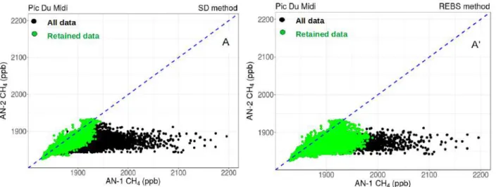
Figure II.8: plots of CH4 measurements of AN-1 against AN-2. All data are in black, and the green

points represent the retained data using SD method for A and REBS method for A’...59

Figure II.9: plots of CO2 measurements of AN-1 against AN-2. All data are in black, and the green

points represent the retained data using SD method for A and REBS method for A’...59

Figure II.10: Number of flagged CO measurements using manual method (blue), SD method (red),

and REBS method (green) for Finokalia (A) and Pic Du Midi (B) ...60

Figure II.11: Example of a spike detection using manual (A), SD (B), and REBS (C) methods

during a known biomass burning event at Finokalia...63

Figure III.1: Diagram of CHIMERE transport model. The boxes represent the different processes.

Cmod and Cobs stand for the modeled and the observed atmospheric concentrations respectively..71

Figure III.2: Normalized temporal profiles of daily, weekly and seasonal variations, applied for

power, industry,residential, processes, and traffic sectors for both CO2 and CH4. The daily

variations are presented in localtime...77

Figure III.3: Simulation domain (red box) and observation sites used in this study. The blue and

green color stand for the atmospheric measurement site (https://icos-atc.lsce.ipsl.fr/) and the

ecosystem measurement sites (https://icos-eco.fr/) respectively. Note that the atmospheric sites are

grouped into four categories according to their characteristics (e.g. topography and environment):

coastal (circle), mountain (triangle), peri-urban (square for GIF only), and tall tower (inversed

triangle)...81

Figure III.4: Panel A, stand for the spatial distribution of the difference between EDGAR and IER

inventories (EDGAR minus IER) for CO2. Panel B (resp. C) represent the cumulated percentages of

the grid cells (resp. national emissions) of the absolute difference between EDGAR and IER for the

metropolitan France. The cumulated percentages are calculated for various classes of CO2

emissions differences...86

Figure III.5: Panel A, stand for the spatial distribution of the difference between EDGAR and IER

inventories (EDGAR minus IER) for CH4. Panel B (resp. C) represent the cumulated percentages of

the grid cells (resp. national emissions) of the absolute difference between EDGAR and IER for the

metropolitan France. The cumulated percentages are calculated for various classes of CH4

emissions differences...87

Figure III.6: Temporal variation of CH4 and CO2 total anthropogenic fluxes over France at a daily

(A and D), weekly (B and E), and monthly scales (C and F). Solid and dashed line represent

respectively the totals for January and July...89

Figure III.7: Monthly totals of NEE fluxes for VPRM and CTESSEL over France...90

Figure III.8: Spatial distribution of the total Net Ecosystem Exchange (NEE) during January and

July, for VPRM (panels A and D), CTESSEL (panels B and E), and VPRM minus CTESSEL

(panels C and F). By convention, a positive sign is a source of CO2 emitted to the atmosphere...92

Figure III.9: Diurnal cycle of the simulated and the observed Net Ecosystem Exchange (NEE) for

four different sites (Barbeau, Grignon, Lamasquere, Puechabon, Figure 3), during January (panel A)

and July (B). The time is presented in UTC...95

Figure III.10: Seasonal cycle of simulated and observed Net Ecosystem Exchange (NEE) at the

four sites (Barbeau, Grignon, Lamasquere, Puechabon)...97

Figure III.11: CO2 average diurnal cycle at BIS, OPE, PUY, TRN, ERS, and GIF, for the observed

Figure III.13: CO2 average diurnal cycle at BIS, GIF, OHP, OPE, PDM, PUY, and TRN, for the

observed (black) and the simulated (red and blue for AROME and ECMWF respectivly)

concentrations during July...103

Figure III.14: CH4 average diurnal cycle at BIS, GIF, OHP, OPE, PDM, PUY, and TRN, for the

observed (black) and the simulated (red and blue for AROME and ECMWF respectivly)

concentrations during July...104

Figure III.15: CH4 daily average at BIS using the nighttime data (00:00 to 06:00) for January (A),

using the afternoon data (12:00 to 18:00) for July (B). The arrows on the top of panels A and B

stand for the wind direction simulated by the AROME (magenta) and ECMWF (cyan).Figure (C)

represent the spatial distribution of the CH4 surface fluxes retreived from EDGARv4.2 FT2010

inventory...105

Figure III.16: CO2 seasonal cycle at BIS, ERS, GIF, OHP, OPE, PDM, PUY, and TRN, for the

observed (black) and the simulated (red and blue for AROME and ECMWF) concentrations. The

monthly mean is calculated using the afternoon data (from 12:00 to 18:00) for low altitude sites and

nighttime data (from 00:00 to 06:00) at the mountain sites...107

Figure III.17: CH4 seasonal cycle at BIS, ERS, GIF, OHP, OPE, PDM, PUY, and TRN, for the

observed (black) and the simulated (red and blue for AROME and ECMWF) concentrations. The

monthly mean is calculated using the afternoon data (from 12:00 to 18:00) for low altitude sites and

nighttime data (from 00:00 to 06:00) at the mountain sites...108

Figure III.18: Spatial distribution of the CO2 monthly differences (ppm) between the CHIMERE

simulations runing with two meteorological models (AROME minus ECMWF), using the data from

12:00 to 18:00 at the first level of the model...110

Figure III.19: Spatial distribution of the CH4 monthly differences (ppb) between the CHIMERE

simulations runing with two meteorological models (AROME minus ECMWF), using the data from

12:00 to 18:00 at the first level of the model...110

Figure III.20: Spatial differences of the simulated boundary layer height (PBL in m) between the

two meteorological models (AROME minus ECMWF), using the data from 12:00 to 18:00...111

Figure III.21: CO2 average diurnal cycle at BIS, OPE, PUY, TRN, ERS, and GIF, for the observed

(black) and the simulated (green and orange for CTESSEL and VPRM respectively) concentrations

during January...115

Figure III.22: CH4 average diurnal cycle at BIS, OPE, PUY, TRN, ERS, and GIF, for the observed

(black) and the simulated (red and blue for IER and EDGAR respectively) concentrations during

January...116

Figure III.23: CO2 average diurnal cycle at BIS, OPE, PUY, TRN, ERS, and GIF, for the observed

(black) and the simulated (green and orange for CTESSEL and VPRM respectively) concentrations

during July...117

Figure III.24: CH4 average diurnal cycle at BIS, GIF, OHP, OPE, PDM, PUY, and TRN, for the

observed (black) and the simulated (red and blue for IER and EDGAR respectively) concentrations

during July...117

Figure III.25: CO2 average seasonal cycle at BIS, ERS, GIF, OHP, OPE, PDM, PUY, and TRN, for

the observed (black)and the simulated (green and orange for CTESSEL and VPRM respectivly)

concentrations. The monthly mean is calculated using the afternoon data (from 12:00 to 18:00) for

low altitude sites and nighttime data (from 00:00 to 06:00) at the mountain sites...120

Figure III.26: CH4 average seasonal cycle at BIS, ERS, GIF, OHP, OPE, PDM, PUY, and TRN, for

the observed (black) and the simulated (red and blue for IER and EDGAR respectivly)

concentrations. The monthly mean is calculated using the afternoon data (from 12:00 to 18:00) for

low altitude sites and nighttime data (from 00:00 to 06:00) at the mountain sites...121

Figure III.27: Spatial distribution of the surface level CO2 monthly differences (ppm) between the

two biogenic models (CTESSEL minus VPRM) panel ΔBio, and between the two anthropogenic

inventories (IER minus EDGAR) panel ΔAnthro, using the data from 12:00 to 18:00 at the first

level of the model...124

Figure III.28: Spatial distribution of the surface level CH4 monthly differences (ppb) between the

two anthropogenic inventories (IER minus EDGAR) panel ΔAnthro, using the data from 12:00 to

18:00 at the first level of the model...125

Figure IV.1 Statistic uncertainty in the Bayesian inversion. The inversion computes the posterior

control vector xa using the observation Y0 and the prior xb. In the classical inversion (top), xa is

estimated together with its uncertainty Pa from the observation and the prior covariance matrices (R

and B). In order to take into consideration the uncertainties in the error statistics, an ensemble of the

couples (R and B) is used to estimate an ensemble of xa and Pa, which stand for p(x|Y0,xb). The

Figure is taken from Berchet. A thesis 2014...138

Figure IV.2: Illustration of the 43 emission regions (colored area) and boundary conditions edges (4

lateral colored dashed lines + 1 top edge) used for the control vector calculation...141

Figure IV.3: Stations providing measurements of CO2 and CH4 during January (left) and July

(right) 2014. Note PDM and OHP sites (south of France) were not available for Janary, and ERS

measurements (located in Corsica) were interrupted during July. the atmospheric sites are grouped

into four categories according to their characteristics (e.g. topography and environment): coastal

(circle), mountain stations (triangle), Peri-urban (square for GIF only), and tall towers (inverse

dtriangle). The red box shows the limit of the model domain...142

Figure IV.4: CH4 hourly data at OPE (left) and PUY (right) in January 2014. The grey color

represents the available observations for each site during January. The back data point stands for the

retained data during the mid-afternoon(data between 14:00 and 18:00) for low altitude sites (OPE),

and the nighttime (data between 00:00 and 06:00) for mountain stations (PUY). The red data show

the observations rejected by the ML algorithm (see section IV.2.3.1)...146

Figure IV.5: Representation of the availability of the CH4 observed data and their contribution to

the inversion for each site. The grey line represents the available data. Black dots stand for the

retained measurements (data between 14:00 and 18:00 for low altitude sites, and data between

00:00 and 06:00 for mountain sites). The color points represent the amount of information used

each day by the inversion system (value 1 indicate that the inversion uses the equivalent of one

hourly data). These information are calculated from the diagonal terms of the sensitivity matrix HK

...148

Figure IV.6: Comparison of the CH4 observation errors calculated by the maximum of likelihood

algorithm (ML) and the absolute difference between the two transport models (ECMWF minus

AROME). The errors are presented using boxes (errors between the 25th and the 75th quantiles),

the horizontal black line for the median, and the mean as shown by the colored dots...150

Figure IV.7: Comparison of the prior flux errors calculated by the maximum of likelihood

algorithm (ML) and the absolute difference between the two anthropogenic maps (EDGAR minus

IER). The errors are presented in percentage according to the monthly fluxes for January (top) and

July (bottom)...152

Figure IV.8: Observed (black) and simulated prior (blue) and posterior (red) CH4 daily averages for

the French atmospheric sites (BIS, GIF, OPE, PUY, TRN, and ERS) during January. The shaded

areas represent the uncertainties of the observed (grey) and simulated prior (shaded blue) and

posterior (shaded red) CH4 concentrations. For each sites we calculate the root mean square error

(RMSE) and the coefficient of correlation (R2) for the prior and the posterior concentration...154

Figure IV.9: Observed (black) and simulated prior (blue) and posterior (red) CH4 daily averages for

Figure IV.10: Spatial distribution of the influence matrices, prior fluxes, the constraint on regions,

and the contribution of the stations for the inversion during January. The constraint map is

generated by convolving the influence matrix KH (presented in the figure by % over the month)

with the prior fluxes. The contribution of the station in the inversion for January is presented using

the diagonal terms of the sensitivity matrix HK. The scales of the constraints maps and the

contribution of the station were chosen arbitrary, in respect with the range of the two maps. The

map in the right (legend map) is presented as a support for number of regions...158

Figure IV.11: Spatial distribution of the influence matrices, prior fluxes, the constraint on regions,

and the contribution of the stations for the inversion during July. The constraint map is generated by

convolving the influence matrix KH (presented in the figure by % over the month) with the prior

fluxes. The contribution of the station in the inversion for July is presented using the diagonal terms

of the sensitivity matrix HK. The scales of the constraints maps and the contribution of the station

were chosen arbitrary, in respect with the range of the two maps. The map in the right (legend map)

is presented as a support for number of regions...159

Figure IV.12: Representation of the posterior error correlation between the 22 constrained regions

during January (left panel), and the 24 constrained region during July (right panel). Because of the

problem of under-constrained regions (section IV.3.1.4), regions 9, 18, 19, and 26 in January, and

regions 1 and 26 in July are not presented. The map in the bottom is displayed as a support for the

region numbers. The regions are grouped into four sectors: North-west (NW), North-east (NE),

South-east (SE), and South-west (SW) sectors, as shown in the legend map and the posterior error

correlation matrices. One sector represents the aggregation of several regions close to each others.

...161

Figure IV.13: Spatial distribution of the monthly uncertainty reduction for the constrained regions

for January (left) and July (right). The uncertainty reduction is presented percentage (%) according

to the prior flux errors...162

Figure IV.14: Panels A (January) and D (July) stand for the monthly total number of groups (y-axis)

of the control vector components independent from initial conditions (IC) and boundary conditions

(BC) for different correlation threshold (the groups may also be formed by only one components). B

(January) and E (July) represent the monthly number of groups formed by at least 2 component of

the control vector independent from IC/BC for several correlation thresholds. The larger the

correlation threshold is, the larger total number of groups is (panels A and D), and the lower number

of groups formed by at two components is (panels B and E), since small number of regions are

correlated together (see section IV.3.1.4). The mean time difference between the component of the

groups (in days) is presented for January (C) and July (F)...164

Figure IV.15: Panels A (January) and C (July) represent the monthly mean area (y-axis) covered by

the groups for each correlation threshold (x-axis). The percentage of the national emissions

constrained by the groups (independent from intitial conditions and boundary conditions) is

presented for January (B) and July (D)...165

Figure IV.16: Total prior (blue) and optimized (red) CH4 emissions over the 27 French regions

during January. The uncertainty related to the prior and optimized emissions are represented by the

error bar. The maps in the bottom can be used as a legend for the number of regions (left) and the

constrained regions (right)...168

Figure IV.17: Total prior (blue) and optimized (red) CH4 emissions over the 27 French regions

during January. The uncertainty related to the prior and optimized emissions are represented by the

error bar. The maps in the bottom can be used as a legend for the number of regions (left) and the

constrained regions (right)...169

Figure IV.18: CO2 hourly data at OPE (left) and PUY (right) during January. The grey color

represents the available observations for each site during January. The back data point stands for the

retained data during the mid-afternoon (data between 14:00 and 18:00) for low altitude sites (OPE),

and the nighttime (data between 00:00 and 06:00) for mountain stations (PUY). The red data show

the observations rejected by the ML algorithm (see section IV.2.3.1)...171

Figure IV.19: Representation of the availability of the CO2 observed data and their contribution to

the inversion for each site. The grey line represents the available data. Black dots stand for the

retained measurements (data between 14:00 and 18:00 for low altitude sites, and data between

00:00 and 06:00 for mountain sites). The color points represent the amount of information used

each day by the inversion system (value 1 indicate that the inversion uses the equivalent of one

hourly data). These information are calculated from the diagonal terms of the sensitivity matrix HK

...172

Figure IV.20: Comparison of the CO2 observation errors calculated by the maximum of likelihood

algorithm (ML, section IV.2.3.1) and the absolute difference of simulated concentration between the

two transport models (ECMWF minus AROME). The errors are presented using whiskers for errors

between the 25th and the 75th quantiles, the horizontal black line for the median, and the colored

dots for the mean observation error...174

Figure IV.21: Comparison of the prior flux errors calculated by the maximum of likelihood

algorithm (ML) and the absolute difference between the two anthropogenic maps (EDGAR minus

IER). The errors are presented in percentage of flux budgets at the monthly scale per region

forJanuary (top) and July (bottom)...175

Figure IV.22: Comparison of the prior flux errors calculated by the maximum of likelihood

algorithm (ML) and the absolute difference between the two anthropogenic maps (VPRM minus

CTESSEL). The errors are presented in percentage of flux budgets at the monthly scale per region

forJanuary (top) and July (bottom)...176

Figure IV.23: Observed (black) and simulated prior (blue) and posterior (red) CO2 daily averages

for theFrench atmospheric sites (BIS, GIF, OPE, PUY, TRN, and ERS) during January. The shaded

areasrepresent the uncertainties of the observed (grey) and simulated prior (shaded blue) and

posterior (shadedred) CO2 concentrations. For each sites we calculate the root mean square error

(RMSE) and thecoefficient of correlation (R2) for the prior and the posterior concentration...178

Figure IV.24: Observed (black) and simulated prior (blue) and posterior (red) CO2 daily averages

for theFrench atmospheric sites (BIS, GIF, OPE, PUY, TRN, OHP, and PDM) during July. The

shaded areasrepresent the uncertainties of the observed (grey) and simulated prior (shaded blue) and

posterior (shadedred) CO2 concentrations. For each sites we calculate the root mean square error

(RMSE) and thecoefficient of correlation (R2) for the prior and the posterior concentration...179

Figure IV.25: Spatial distribution of the influence matrices, prior fluxes, the constraint on regions,

and the contribution ofthe stations for the inversion in January. The constraint map is generated by

convolving the influence matrix KH(presented in the figure by % over the month) with the prior

anthropogenic emissions. The contribution of the station in the inversion forJanuary is presented

using the diagonal terms of the sensitivity matrix HK. The scales of the constraints maps and

thecontribution of the station were chosen arbitrary, in respect with the range of the two maps. The

map in the right(legend map) is presented as a support for number of regions...181

Figure IV.26: Same as figure 25 in July (anthropogenic fluxes)...182

Figure IV.27: Same as figure 25 for biogenic fluxes...183

Figure IV.28: Same as figure 27 in July (biogenic fluxes)...183

Figure IV.29: Panel A (January) and E (July) represent the posterior error correlation between the

constrained anthropogenic emission regions in France (section IV.3.2.4). Panel D (January) and H

(July) represent the posterior error correlation between the constrained biogenic flux regions in

shown in the legend map and the posterior error correlation matrices. One sector represents the

aggregation of several regions close to each others...186

Figure IV.30: Spatial distribution of the monthly uncertainty reduction for the constrained

anthropogenic emission (CO2 anthro) and biogenic fluxes (CO2 Bio) for January and July. The

uncertainty reduction is presented in percentage (%) according to the prior flux errors...187

Figure IV.31: Panels A (January) and C (July) stand for the monthly total number of groups (y-axis)

of the control vector components independent from initial conditions (IC) and boundary conditions

(BC) for different correlation threshold (the groups may also be formed by only one component). B

(January) and D (July) represent the monthly number of groups formed by at least two components

of the control vector independent from IC/BC for several correlation thresholds. The larger the

correlation threshold is, the larger total number of groups is (panels A and C), and the lower number

of groups formed by at two components is (panels B and D), since small number of regions are

correlated together (see section IV.3.2.5)...189

Figure IV.32: Panels A (January) and D (July) represent the monthly mean time difference (in days)

calculated between the component of the groups for the anthropogenic emissions. Panels B

(January) and E (July) stand for the percentage of the anthropogenic emissions constrained by the

groups formed independently from initial conditions (IC) and boundary condition (BC). Panels C

(January) and F (July) display the monthly mean area covered by the groups without IC/BC for the

anthropogenic emissions...190

Figure IV.33: Same as figure 32 for the biogenic fluxes...191

Figure IV.34: Total prior (blue) and optimized (red) anthropogenic CO2 emissions over the 27

French regions during January. The uncertainty related to the prior and optimized emissions are

represented by the error bar. The maps in the bottom show the number of regions (left) and the

constrained regions (right)...194

Figure IV.35: Same as figure 34 for July...195

Figure IV.36: Total prior (blue) and optimized (red) biogenic CO2 emissions over the 27 French

regions during January. The uncertainty related to the prior and optimized emissions are represented

by the error bar. The maps in the bottom show the number of regions (left) and the constrained

regions (right)...198

Figure IV.37: Total prior (blue) and optimized (red) biogenic CO2 emissions over the 27 French

regions during July. The uncertainty related to the prior and optimized emissions are represented by

the error bar. The maps in the bottom show the number of regions (left) and the constrained regions

(right)...199

Figure V.1: A) Count of the CO2 contaminated data by wind direction at OPE. The count is

represented by grey circles (first circle=50 data, the second=100, and the third=150 data). The

colors stand for the difference between contaminated data (Ci) and the last uncontaminated data

(Cunf), using the SD method. B) represents a Google earth image of the OPE area...209

Figure V.1: A) Count of the CO2 contaminated data by wind direction at OPE. The count is

represented by grey circles (first circle=50 data, the second=100, and the third=150 data). The

colors stand for the difference between contaminated data (Ci) and the last uncontaminated data

(Cunf), using the SD method. B) represents a Google earth image of the OPE area...211

Tables

Table II.1: Measurement sites characteristics...45

Table II.2: Sensitivity of SD method spike detection for two sets of α (α=1 and α=3), and for two

range of background data interval (σb and σt scenario) for the four stations and all species...49

Table II.3: Sensitivity of REBS spike detection method for two sets of(β =3 and β =8) for the four

stations and all species for the year 2015.Based on these sensitivity tests for the SD and REBS

parameters, and the a prior estimation of the percentages of spikes manually detected by site

managers, we apply the SD method with σb and α = 3 for CO and with σb and α = 1 for CO2 and

CH4. For the REBS method we use β = 8...51

Table II.4: percentage (rounded to one decimal) and number of contaminated data detected by SD,

REBS, and COV method overall stations (AMS, FKL, OPE and PDM) and for the three species

CO, CO2 and CH4.Generally, the methods SD and REBS automatically detect spikes. However, the

COV method requires a prior knowledge of datasets and the approximate number of data to be

filtered. Because of this limitation for automatic spike detection we have discarded the COV

method from further tests for the selection of the most reliable method for spike detection...53

Table II.5: percentages and number of contaminated data detected by SD, REBS methods for CO2

and CH4 at PDM...54

Table II.6: Classification of the number of hours in which the SD method filtered at least

one-minute data point for CO, CO2, and CH4 at the four sites. The intervals represent the differences

between filtered and the non-filtered time-series averaged at a hourly scale in (ppm) for CO2 and

(ppb) for CO, and CH4. The values in brackets represent the percentages of the impacted hours on

the whole time-series...64

Table III.1: Main characteristics of the CHIMERE configuration used in this study. (-) means that

no biogenic fluxes were used for CH4...71

Table III.2: Table linking the UNFCCC categories of emissions and the activity sectors for which

the temporal profiles are defined in the LOTOS EUROS project

http://www.eea.europa.eu/publications/EMEPCORIN-AIR5. For example the temporal factor of the

industry sector is applied to the UNFCCC category 1A1+1A2 (Energy manufacturing

transformation)...74

Table III.3: Atmospheric stations characteristics. The altitude of the site represents the altitude of

the ground above sea level at the site location, and the inlet height is the altitude of the inlet above

ground level. The type of sites are classified according to the topography. (-) means that

corresponding sites are recent and still not published...81

Table III.4: Ecosystem stations used in this study...82

Table III.5: Comparison of the rescaled annual anthropogenic emissions for metropolitan France

from IER, EDGARv4.2 and CITEPA (SECTEN format) inventories for the year 2014. In order to

make the CITEPA data easily understandable the anthropogenic emission are prepared using the

SECTEN format (SECTeurs Economiques et éNergie). (1) means that emissions are separated

according to Energy and the Economic sectors (SECTEN format)...83

Table_IV. 1: Characteristics of the surface fluxes used as prior in the inverse framework. (*) means

that the corresponding fluxes were produced using hourly temporal profils applied on the yearly

totals (Section III.2.3)...144

Table IV.2: Inversion results of total prior and optimized fluxes over France, and over the four

sectors: the North-west (NW), the North-east (NE), the South-east (SE), and the South-west (SW).

The limits of these sectors can be found in the legend map Figure IV.16...167

Table IV.3: Inversion results of total prior and optimized CO2 anthropogenic fluxes over France,

and over the four sectors: the North-west (NW), the North-east (NE), the South-east (SE), and the

South-west (SW). The limits of these sectors can be found in the legend map Figure IV.34...193

Table IV.4: Inversion results of total prior and optimized CO2 biogenic fluxes over France, and over

the four sectors: the North-west (NW), the North-east (NE), the South-east (SE), and the South-west

(SW). The limits of these sectors can be found in the legend map Figure IV.36...197

Chapter I:

Introduction

I.1

Global radiative balance:

The Earth receives an energy of 340 W.m-2 _{from shortwave solar radiation (Figure I.1). 30% of this energy is} directly reflected back to space by clouds, aerosols, and the earth surface. The remaining part of the incident shortwave radiation (185 W.m-2_{) is absorbed by the atmosphere and earth's surface. This energy will be} reemitted afterward by the earth system in longwave radiation (e.g., sensible and latent heat, and thermal energy). The latent heat (around 84 W.m-2_{) is associated to the evaporation of water at the Earth surface,} whereas the sensible heat (around 20 W.m-2_{) stands for the heat transfer by conduction between the Earth} surface and the atmosphere. In addition to these fluxes, the Earth emits infrared radiation (398 W.m-2_{), in the} form of thermal energy. 60% of the total infrared flux (239 W.m-2_{) is re-emitted directly to space, while the} remaining part is absorbed by greenhouse gases (H2O, CO2, and CH4). This later contribution (342 W.m-2) of infrared radiations to the Earth system (Figure I.1), known as the greenhouse effect, leads to the increase in global temperature.

Without the natural greenhouse effect, the mean temperature at the Earth surface would be -18° Celsius (C) instead of +15° C. This indicates that the natural greenhouse effect ensures a warming of 33°C, making life possible on Earth. In order to maintain this natural warming, the total of energy absorbed and emitted by the Earth system must be zero. However, the emission of additional greenhouse gases in the atmosphere by the human activities, causes an energy imbalance of 0.8±0.2 W.m-2 _{(Trenberth et al, 2009), which leads to the} global warming of the atmosphere.

Since 1990 the Intergovernmental Panel on Climate Change (IPCC) demonstrated that human activities have modified significantly the Earth temperature compared to the pre-industrial period (5th Assessment Report of the IPCC 2013). In fact, the enhancement of the earth radiative energy imbalance contributes to the increase

I.2

Role of the greenhouse gases in global warming

Since the industrial revolution, human activities have been injecting into the atmosphere important quantity of carbon dioxide (36183 MtCO in 2016, according to Global Carbon Atlas, www.globalcarbonatlas.org/)₂ and other greenhouse gases such as methane (CH4) and nitrous oxide (N2O). The CO2 emissions are mainly related to fossil fuel combustion for industrial, domestic and transport energy needs. CH4 is mostly linked to agricultural practices (e.g., rice growing and enteric fermentation), waste decomposition, as well as oil and gas production. Whereas, N2O is emitted mostly from agricultural activities, with the use of mineral and animal fertilizers. Other new substances such as the Chlorofluorocarbons (CFC), hydrochlorofluorocarbons (HCFC), whose origin is totally anthropogenic, are characterized by a greenhouse gas effect that may exceed thousands of times the one of CO2 (Flanner et al., 2018). All these gases alter the global energy balance leading to the additional energy trapping near the surface. Other atmospheric components, such as aerosols, have a negative radiative forcing, which may lead to the atmospheric cooling (Figure I.2)

Figure I.1 : Global radiative balance in the current climate. The numbers in bold correspond to the estimate of each energy flux in W.m-2 _{(5th Assessment Report of the Intergovernmental Panel} on Climate Change 2013)

The contribution of the main greenhouse gases to the radiative forcing is presented in figure I.2. Since the beginning of the pre-industrial era, the additional radiative forcing caused by the anthropogenic activities is estimated to 2.3 W.m-2 _{(between 1.1 to -3.0 W.m}-2_{, Myhre et al., 2013). According to the 5th Assessment} Report of the IPCC (IPCC 2013), the CO2 is responsible for the highest radiative forcing that exceeds 1.5 W.m-2 _{(Figure I.2). CO}

2 contributes by more than 50% to the additional radiative forcing produced by the greenhouse gases, whereas the CH contribution is about 20%. The impact of the other atmospheric

Figure I.2: Radiative forcing of the main anthropogenic (greenhouse gases, aerosol, short-lived gas) and natural (solar radiation) factors impacting the climate in 2011 compared to 1750 (5th

gases, we use the Global Warming Potential index (GWP). This index has been developed by Houghton and Jenkins (1990) in order to quantify the greenhouse effect of each gas compared to CO2. Greenhouse gas emissions are often calculated based on the amount of CO2 that would be required to produce a similar warming effect over a given time period. This is calculated by multiplying the amount of the emitted gas by its corresponding GWP index. The CO2 represents the reference value with a GWP index equal 1. For CH4, Etminan et al., (2016) estimated a GWP index 32 times higher than CO2 over a 100 year time period. The GWP index of N2O is estimated to 260 for the same period (Etminan et al., 2016).

I.3

Carbon budget

I.3.1 Carbon dioxide cycle

CO2 is the subject of many exchanges between land, ocean, and atmosphere. Figure I.3 represents the main carbon fluxes between the different reservoirs constituting the global carbon cycle.

The atmospheric concentrations of CO2, which was 280 ppm (parts per million by volume) during the pre-industrial era, increased to 380 ppm in 2011 (IPCC, 2013), and exceeded an average of 410 ppm across the entire month for the first time at Mauna Loa in last April. The rise of atmospheric CO2 concentrations is mainly related to the emissions by fossil fuel combustion estimated to 9.4 ± 0.5 GtC/yr (Le Quéré et al., 2017). The second largest anthropogenic source results from the land use changes, in particular, the deforestation estimated to 1.3 ± 0.7 GtC/yr (Le Quéré et al., 2017).

As shown in figure I.3, the global carbon cycle links together the atmosphere, the oceans, the land, and the fossil fuel reservoirs. The carbon fluxes are distributed, between these reservoirs, in different proportions. For example, the carbon fluxes between the atmosphere and the land are exchanged in both directions. The carbon is absorbed by the biomass due to the photosynthesis processes (123 PgC/year), and returns back to the atmosphere by surface emissions, fires, as well as plant, animal and microorganism respirations.

The fluxes represented by black arrows on the figure I.3 show the net fluxes estimated for the pre-industrial era. The red arrows represent the additional fluxes emitted on average in the decade 2000-2009 by the human activities, including fossil fuel burning, land use changes and cement production. The additional anthropogenic carbon fluxes are estimated to 9 PgC/year. Of these 9 PgC/year, about 5 are absorbed by land and oceans, and 4 remain in the atmosphere, leading to the increase of the CO2 atmospheric concentrations which is precisely monitored at background observatories (Prather et al., 2012). If the magnitude of the oceanic and terrestrial sources and sinks are relatively well known on a global scale, their contributions at the sub-continental scale remain largely uncertain.

Figure I.3: Representation of the carbon cycle. The annual fluxes are estimated in PgC/year and averaged over the period 2000-2009. The amount of CO2 stored in the three reservoirs is expressed in PgC. The figure is taken from the 5th assessment report of the intergovernmental panel for the Climate Change (IPCC 2013)

I.3.2 Methane cycle

During the pre-industrial era, the methane atmospheric concentration was about 700 ppb (parts per billion by volume), with a total emission of 215 TgCH4/year (Lelieveld et al., 2002). Since 1750, CH4 atmospheric concentrations increased by 150% (from 700 ppb) to a global mean value of 1853±2 ppb in 2016 (WMO Greenhouse Gas Bulletin N.13). The methane emissions can be separated into three types: natural, pyrogenic, leakages:

• Natural emissions are the result of fermentation reactions and methanogenesis processes of some microbes, produced from organic matter under low oxygen conditions. This category includes emissions from wetlands (e.g., peatlands, swamps, rice fields), termites, animals, landfill sites, wastewater, ruminants.

 Pyrogenic sources result from incomplete combustions, from biomass fires or fossil fuels such as domestic biofuels.

 Leakage emissions are caused by fossil fuel extraction and use (e.g., coal, natural gas, and oil industry).

The relative proportions of the different CH4 sources were estimated by Dlugokencky et al (2011) as presented in figure I.4, and recently revised by Saunois et al., (2016). The methane natural emissions were estimated to 218±47 TgCH4/year, whereas the anthropogenic emissions were estimated to 335±68 TgCH4/year. The anthropogenic activities include emissions from agriculture, waste treatment, biomass fires, transportation and fossil fuels combustion. At the global scale, the highest contribution was determined for wetlands with a total ranging between 177 and 284 TgCH4/year. The contributions of the geological sources, termites, hydrates and freshwater emissions are estimated respectively to 54±21, 12±10, 5±3, and 40±23 TgCH4/year. For the anthropogenic emissions, the most important contributions come from fossil fuels, waste management, rice and farming estimated to 95±10, 78±12, 37±3, 90±4 TgCH4/year respectively. The comparison between these sources showed the significant impact at the global scale of the wetlands, followed by the anthropogenic emissions. However, over the regional domain studied in this thesis (metropolitan France) some emissions, like the wetlands, biomass burning, rice cultivation, are much less important and can be neglected (Champeaux et al., 2005).

I.4

CO

and CH

atmospheric measurerments

Direct measurement of the greenhouse gases has begun in 1958 by the sampling of the atmospheric concentrations of CO2 at Mauna Loa (Hawai, USA) with the initiative of C. D. Keeling (Keeling, 1960). Measurement networks have been gradually expanded around the world and extended to other greenhouse gases, including the methane since 1978 (Blake et al., 1982, Dlugokencky et al., 1994), with the objective to

Figure I.4: Representation of the methane cycle. The annual fluxes are estimated in TgCH 4/year and averaged over the period 2000-2009. The amount of CH4 stored in the three reservoirs is expressed in TgCH4. This figure is taken from the 5th assessment report of the intergovernmental panel for the Climate Change (IPCC 2013)

networks distributed around the world (Figure I.5). Two types of approaches are commonly adopted for the atmospheric sampling of the greenhouse gas concentrations:

 Continuous measurements by in-situ instruments: this approach is based on direct measurements using instruments at surface sites or on mobile platforms (aircraft, ships). The main advantage of the continuous measurements relays on the ability to investigate the atmospheric variations at short term scales. The development of laser-based optical measuring instruments has allowed a strong development of measurement sites over the last 10 years.

 Flask sampling coupled with in-lab analysis: such monitoring programs are generally developed at a frequency of few samples per month, which allows the characterization of long term trends and seasonal variations at background sites. The main advantage of the flask sampling is the possibility to perform multi-species measurements with limited infrastructure in the field.

Figure I.5 distinguishes several measurement networks. Panels a) and b), retrieved from the Earth System Research Laboratory website (https://www.esrl.noaa.gov/gmd/ccgg/globalview/), show the collaborative monitoring network led by NOAA/ESRL (USA). AGAGE (Advanced Global Atmosphere Gases Experiment) is also one of the oldest networks, providing measurements of different greenhouse gases (but not CO2) since the beginning of the 1980s (Prinn et al., 2000; Cunnold et al. 2002). More recently, regional networks have also been developed, such as the RAMCES network in France presented in panel c) (Yver et al., 2011). The European Research Infrastructure network ICOS (Integrated Carbon Observation System, https://www.icos-ri.eu/icos-national-networks) aims to develop a dense and standardized monitoring network in Europe. Several data retrieved from the RAMCES and ICOS networks are used in this thesis.

The increasing number of measurement sites has made possible the development of methods dedicated to the estimation of the CO2 and CH4 surface fluxes at increasingly finer spatial scales (Bergamaschi et al., 2018, Kountouris et al., 2018).

I.5

Flux estimation approaches :

inventories are reported every year by the countries to the United Nations Framework Convention on Climate Change (UNFCCC) and form the official data for international climate policies. In France, this activity is compiled by the Centre Interprofessionnel Technique d'Etudes de la Pollution Atmosphérique (CITEPA). Emissions are classified into different sectors (agriculture, transport, energy industries, residential, manufacturing combustion, industrial processes, waste, etc…), and their estimates must follow the guidelines established by the Intergovernmental Panel on Climate Change (IPCC). Similar activities are performed more and more frequently at regional and city scales. The bottom-up approach has significant uncertainties due to the incomplete accounting of all emitting sectors, and by the large uncertainties in the emission factors and activity statistics for many source sectors.

The greenhouse gases inventories currently reported by UNFCCC do not provide a complete picture of the global emissions since not all countries report their emissions every year. For this reason, comprehensive and consistent inventories are developed in addition to the national inventories reported to UNFCCC. This is for example the case of the Emissions Database for Global Atmospheric Research (EDGAR) (Janssens-Maenhout et al., 2017), which estimate anthropogenic emissions for all world countries (e.g. EDGARv4.3.2 FT2012 inventory available at http://edgar.jrc.ec.europa.eu/), or the European inventory provided by Institute for Energy Economics and the Rational Use of Energy (IER), University Stuttgart. Such inventories also have the advantage of providing information on regular spatial grids, which can be used as an input to the atmospheric simulations.

The inventories, like EDGAR or IER, generally do not cover all natural emission processes, like for example the CO₂ exchange with the terrestrial ecosystems due to the plant and soil respiration, or the carbon uptake due to the photosynthesis. For those sectors, we may use biogeochemical models which often used remote sensing observations of the state of the vegetation and the weather. Such models are themselves validated by using direct measurement of atmospheric fluxes, which are very local and representative of an area less than 1 km2 (Schmid et al., 1994). Due to the strong spatio-temporal heterogeneities of the fluxes, the extrapolation of such measurements using biogeochemical models still faces significant uncertainties.

I.5.2 Top-down approach

The top-down approach provides an estimation of the surface fluxes using measured atmospheric concentrations, atmospheric models, and prior information of the surface fluxes. In this thesis, the

quantification of the CO2 and CH4 fluxes over France will be performed using the Bayesian top-down approach (Tarantola et al. 2005) called hereafter by the inverse modelling. The robustness of this approach depends on the quality of the transport model that mix and transport the surface fluxes to be comparable with the measured concentration. The atmospheric concentration of a given gas represents the amount of fluxes transported in the atmosphere through different processes (e.g. horizontal and vertical mixing). As shown by Peylin et al (2002), the estimation of the CO2 fluxes at the regional scale can be uncertain in case of important transport errors. Consequently, the first step before the development of any inverse modelling framework should be the evaluation of the quality of the transport model used to build our inverse system.

The top-down approaches represent thus a powerful tool to evaluate and verify the emission inventories provided by the bottom-up approach (Marquis et al., 2008). Previous studies showed significant differences between the top-down and the bottom-up GHG estimates (Bergamaschi et al., 2018, Kountouris et al., 2018, Le Quéré et al., 2015, Saunois et al., 2016). For example, the long term atmospheric measurements of sulfur hexafluoride (SF6), an industrial gas with an atmospheric lifetime of about 850 years, suggested an under-estimation of the SF6 emissions reported by countries to UNFCC by a factor of two (Levin et al., 2010). Several studies have demonstrated in recent years that atmospheric measurements of CO2 and CH4 can be used to quantify top-down continental emissions in Europe and the United States, where the monitoring networks are the densest. This was the case for example for Bergamaschi et al (2018) who estimates higher CH4 emissions for the European countries compared to the bottom-up inventories.

I.6

Estimation of the regional fluxes

I.6.1 Some techniques for flux optimization

During the last two decades, the top-down approaches, known also by flux inversion, have been largely used for the estimation of the GHG surface fluxes at the global (e.g. Enting et al., 1995; Kaminski et al., 1999a; Gurney et al., 2003; Locatelli et al., 2013), and the regional scale (e.g. Gerbig et al., 2003; Peylin et al., 2005; Lauvaux et al., 2012; Broquet et al., 2013, Berchet et al., 2014, Bergamaschi et al., 2018, and Pison et al., 2018). Several techniques have been developed with the aim to estimate the surface flux patterns at a

weekly time scale by separating between daytime and night-time data. Lauvaux et al (2012) resolved the problem using the Bayesian inversion approach for matrice solution based on an analytical framework (Tarantola, 2005). Using the same Bayesian approach, Bréon et al (2015) and Staufer et al (2016) performed a flux inversion in order to estimate the anthropogenic CO2 emissions using the atmospheric measurements at a sub-national scale in France. For this thesis, we have used a similar Bayesian approach applied to the national inventory of CO2 and CH4 emissions over France, where we are benefiting from the recent development of the atmospheric monitoring network as part of the Europeans research infrastructure ICOS.

I.6.2 Estimation of CO

fluxes

Using the Bayesian inversion framework, a compilation of three mesoscale and two global transport models, was performed in order to estimate the European CO2 fluxes from three atmospheric inversion frameworks (Rivier et al., 2010). In this work, the authors demonstrate that the European continent could be split in a CO2 sink for all western and southern European countries, and a CO2 source for the central and Eastern Europe (Figure I.6). In this study, the five inversion systems were in good agreement to estimate a sink of about -1 GtC/year for western and southern Europe, a CO2 source of less than 0.8 GtC/year for Central Europe, and less than 0.2 GtC/year for Eastern Europe (Figure I.6). In a more recent study, Kountouris et al., (2018) estimate the biogenic carbon fluxes for Europe using seven high-resolution regional inversion systems. The result of this study confirms the CO2 sink over Europe with a value that may reach -0.71 GtC/year as presented in figure I.7. The two studies estimated the annual CO2 budget in Europe with significant uncertainties, which may reach more than 50%. This indicates that our knowledge of the biospheric CO2 flux estimate in Europe remains uncertain.

The comparison between the regional inversion results of Kountouris et al (2018) and earlier studies (Ciais et al., 2000, Gurney et al., 2004, Rivier et al., 2010, Peylin et al,. 2013, Reuter et al,. 2014) confirms the high uncertainty of the European CO2 surface fluxes (Figure I.7). The estimated fluxes from Kountouris et al., (2018) range between -0.23±0.13 GtC/year and -0.38±0.17 GtC/year, and reach -0.55±0.2 GtC/year for the TransCom European region as defined in Gurney et al (2002). For the earlier studies the estimated fluxes vary between -0.3±0.8 GtC/year for the period 1985-1995 (Ciais et al., 2000) and -1.1±0.3 GtC/year for the year 2007 (Reuter et al., 2014). The significant differences between the different studies can be related to the high interannual variability of the surface fluxes as demonstrated by Broquet et al (2013). The first inverse modelling of CO2 have focused on the natural CO2 fluxes, which have much larger uncertainties than the anthropogenic CO emissions. In thoses studies it is commonly assumed that the uncertainty of fossil fuel