The WC10 central stars CPD−56° 8032 and He 2-113 -III. Wind electron temperatures and abundances

Mon. Not. R. Astron. Soc. 297, 999–1014 (1997)

The WC10 central stars CPD

Ð56° 8032 and He 2–113 –

III. Wind electron temperatures and abundances

Orsola De Marco,

P. J. Storey

and M. J. Barlow

1_{Department of Physics and Astronomy, University College London, Gower Street, London WC1E 6BT} 2_{Institut f¨ur Astronomie, ETH Zentrum, H¨aldeli-Weg 15, CH-8092 Z¨urich, Switzerland}

Accepted 1998 January 27. Received 1998 January 19; in original form 1997 September 25

A B S T R A C T

We present a direct spectroscopic measurement of the wind electron temperatures and a determination of the stellar wind abundances of the WC10 central stars of planetary nebulae CPDÐ56° 8032 and He 2–113, for which high-resolution (0.15-Å) UCLES echelle spectra have been obtained using the 3.9-m Anglo-Australian Telescope.

The intensities of dielectronic recombination lines, originating from autoionizing resonance states situated in the C2++eÐ continuum, are sensitive to the electron temperature through the populations of these states, which are close to their LTE values. The high-resolution spectra allow the intensities of fine-structure components of the dielectronic multiplets to be measured. New atomic data for the autoionization and radiative transition probabilities of the resonance states are presented, and used to derive wind electron temperatures in the two stars of 21 300 K for CPDÐ56°8032 and 16 400 K for He 2–113. One of the dielectronic lines is shown to have an autoionization width in agreement with the theoretical predictions. Wind abundances of carbon with respect to helium are determined from bound–bound recombination lines, and are found to be C/He\0.44 for CPDÐ56° 8032 and C/He\0.29 for He 2–113 (by number). The oxygen abundances are determined to be O/He\0.24 for CPDÐ56° 8032 and 0.26 for He 2–113.

The effect of optical depth on the temperature and abundance determinations is investigated by means of a Sobolev escape-probability model. We conclude that the optically thicker recombination lines can still be used for abundance determinations, provided that their upper levels are far from LTE.

Key words: atomic data – stars: AGB and post-AGB – stars: individual:

CPDÐ56° 8032 – stars: individual: He 2–113 – stars: Wolf–Rayet – planetary nebulae: general.

1 I N T R O D U C T I O N

Of all central stars of planetary nebulae (CSPNe), about 10–15 percent are of Wolf–Rayet type (WR). They have little or no hydrogen in their atmospheres, are composed mainly of helium, carbon and oxygen, and possess a fast, dense and extended stellar wind. Their spectra can mimic the spectra of massive (150 M_>) Population I WR stars of the carbon sequence (WC), despite having a completely different evolutionary history. The low-excitation WR cen-tral stars are thought to mark the beginning of the

evolu-tionary tracks of hydrogen-deficient central stars. Because of their key position, knowledge of their stellar and wind parameters is critical. Amongst the [WCL]1

stars, those in the [WC10] and [WC11] classes have not yet developed the fast winds that blend spectral features in the hotter [WC9] and [WC8] central stars. This means that most line compo-nents are resolved, greatly facilitating direct spectral line

1

The [ ] notation was introduced by van der Hucht et al. (1981) to distinguish the WR central stars of PNe from massive WR stars, and the letter ‘L’ stands for ‘late’.

analysis. CPDÐ56° 8032 and He 2–113 have been classi-fied as [WC10] (Webster & Glass 1974; De Marco, Barlow & Storey 1997, hereafter Paper I; Crowther, De Marco & Barlow 1998). To date four WR CSPNe definitely populate the WC10 class, namely CPDÐ56° 8032, He 2–113, M4-18

and IRAS 17514Ð1555 (PM 1–188). One star, K 2–16, has

a cooler spectrum and is put as the sole representative of the [WC11] class by Crowther et al. CPDÐ56° 8032 was first recognized as a cool carbon WR star by Bidelman, MacCon-nel & Bond (1968), while He 2–113 was found to be an emission-line star by Henize (1967).

In this paper we describe a method for the determination of the electron temperature in the CIIline-forming region. In a previous effort to determine the wind electron tem-perature of [WC10] stars, Barlow & Storey (1992) analysed

a spectrum of CPDÐ56° 8032 taken with the RGO

Spec-trograph on the 3.9-m Anglo-Australian Telescope (AAT) at a resolution of 0.98Å(red) and 0.50Å(blue) in first and second order. The higher resolution UCLES echelle spectra used in this paper allows much more reliable deblending of

the components of the CII dielectronic multiplets. This

paper is the third in a series aimed at developing a detailed

analysis of the [WC10] stars CPDÐ56° 8032 and He 2–113.

In Paper I we carried out an empirical nebular analysis, while in Paper II (De Marco & Crowther 1998) stellar and nebular modelling was presented. In this paper we present, along with the direct determination of the wind electron temperatures, a determination of the wind abundances, and assess the quality of the results by developing a detailed optical depth analysis and by comparing this with the wind modelling from Paper II.

Neither of the two echelle spectra is displayed here in its entirety, but they will be presented, together with complete line identifications, by De Marco et al. (in preparation).

In Section 2 we give a short summary of the observations and data reduction (a full account is given in Paper I). Section 3 explains the method by which the wind electron temperature can be inferred from low-temperature dielec-tronic recombination lines. The atomic data used in the calculations are described in Section 4. In Section 5 the fits that allowed us to determine the fluxes in the dielectronic recombination lines are explained. The wind electron

tem-peratures for the C2+ line-forming regions are finally

derived in Section 6. In Section 7 we derive the stellar wind abundances of carbon and oxygen with respect to helium. In Section 8 we consider optical depth and its effects on the fluxes of recombination lines. We summarize our results in Section 9.

2 O B S E RVAT I O N S , D ATA R E D U C T I O N A N D R E D D E N I N G

CPDÐ56° 8032 and He 2–113 were observed with the AAT

on 1993 May 14 and 15 using the 31.6 line mmÐ1 UCL

Echelle Spectrograph (UCLES) with a 1024Å1024 pixel

Tektronix CCD as detector. Four settings of the CCD were needed in order to cover the entire echellogram: two adja-cent ones in the far-red and two in the blue. Complete

wavelength coverage was obtained from 3600 to 9200Å. At

each wavelength setting we obtained 5-arcsec wide-slit spec-tra for absolute spectrophotometry and 1.5-arcsec narrow-slit spectra for maximum resolution (R\50 000). The

continuum signal-to-noise ratios ranged from 20 to 60, depending on exposure time, the brightness of the object and the system spectral response. A log of the observations, together with details of the data reduction, was presented in Paper I.

The reddening was derived (in Paper I) from the

observed nebular Ha/Hb decrement, as well as from the

ratio of the radio-free–free and Hb fluxes. We found that

E(BÐV)\0.68 for CPDÐ56° 8032 and 1.00 for He 2–

113.

3 D E T E R M I N AT I O N O F T H E W I N D E L E C T R O N T E M P E R AT U R E : M E T H O D

Many of the lines in the spectra of WC stars are excited primarily by recombination processes. Of these, some are due to the process of low-temperature dielectronic recombi-nation (Storey 1981; Nussbaumer & Storey 1984). Such lines arise from quasi-bound autoionizing states lying at energies above the ionization limit of the ion in question. These states are formed by dielectronic capture from the continuum, and decay either by radiative transitions to other states (autoionizing or bound) or by radiationless transitions back to the continuum (autoionization). The latter process usually dominates, and the population of the states is given by the Saha equation. We are concerned with dielectronic lines that arise from transitions directly from

autoionizing states. In CPDÐ56° 8032 and He 2–113 four

dielectronic multiplets have been detected arising from C+.

We assume initially that the electron temperature for the region of formation of CIIrecombination lines is constant, and that the dielectronic lines are optically thin. However, as we will see in Section 8, the assumption of optical thin-ness can be relaxed as long as we compare lines of similar optical thickness. The population of an autoionizing state can be expressed as Nu NeNi \ wu 2w₊

2

3

2

3

where Nuis the population density of the upper state, Neand

Ni are the electron and ion densities, wu and w+ are the

statistical weights of the upper (autoionizing) state and of the recombining ion ground state (C2+ 1S, w₊\1) respec-tively, Euis the energy of the autoionizing state with respect

to the C2+ 1S ground level, Teis the wind electron

tempera-ture of the CIIline-forming region, and the other quantities have their usual meaning. The factor bumeasures the

depar-ture of the population of the state from its thermodynamic equilibrium value and is given by

bu\ GA u GA u+G R u , (2) where GA

uis the autoionizing probability, and G R

uis the total

radiative decay probability.

The emissivity in each transition is given by

e\NuG R

ulhvul, (3)

where GR

ul is the transition probability to a specific lower

observed at the Earth is given by

F(lul)\

1

4pD2

h

where V is the emitting volume, and D is the distance to the source. By comparing the fluxes in lines of sufficiently

dif-ferently Eu we can determine the electron temperature

directly. By combining equations (1), (2), (3) and (4) we have F(l, Te)\Q(l, Te)Å 1 4pD2

h

2

3

2

3

where I(l) is the measured dereddened flux in the line of

wavelength l. If our stated assumptions were correct and

the flux measurements were free of error, we would obtain the same value of X(l, Te) from each of the four transitions

at the electron temperature of the emitting region. Since the data have errors, we calculate a weighted mean, ¯X(Te), from

the four transitions, making use of the uncertainties in the observed fluxes. We then vary Teto minimize

x2 \+ 4 i\1

&

'

where siis the error on X(li, Te). In this way we obtain an

estimate of the electron temperature consistent with the fluxes and errors of all four transitions. We also obtain an estimate of the error on the temperature by determining those temperatures for which x2

changes by unity from its minimum value.

4 T H E C2+++ _{AT O M I C D ATA}

The four CIImultiplets of interest are shown in the Gro-trian diagram in Fig. 1. The fine structure of the initial and final terms separates each multiplet into three components for multiplets 50, 51 and 28.01 and four components for multiplet 25, whose separations are approximately compar-able to the linewidths.

The energies relative to the ionization limit are taken from Moore (1970). For each upper level we require the

departure coefficient, bu, given by equation (2). The

autoionization and radiative lifetimes needed to calculate bu

are given in Table 1. The autoionization probabilities were

derived from a C2++eÐ scattering calculation by Davey

(1995), in which the autoionizing states appear as reso-nances in the calculated photoionization cross-section. The probabilities GA

uwere obtained by fitting these resonances to

Fano profiles. The calculation by Davey (1995) was carried out in LS coupling and neglects all relativistic energy shifts and fine-structure interactions (spin–orbit, etc.). This is a good approximation for the 3dp2_Po_and 2_Fo_{terms, but not}

for the 4fp terms, where these interactions are stronger. We have therefore carried out an atomic structure calculation

using the program SUPERSTRUCTURE (Eissner, Jones &

Nussbaumer 1974; Nussbaumer & Storey 1978), which incorporates these effects. The calculation, which includes all terms of the two electron configuration 2s2p3d and 2s2p4f, incorporates the spin–orbit interaction and the two-body fine-structure interactions described by Eissner et al. The electron radial wavefunctions are calculated in scaled Thomas–Fermi–Dirac potentials, with the scaling param-eters being determined by making the statistically weighted Figure 1. Grotrian diagram of the energy levels of the CII

autoio-nizing lines.

Table 1. Summary of the atomic data used to analyse dielectronic lines. Euis the energy of the upper state relative to the ground level of C2+_.

sum of all the term energies a minimum. The electrostatic Hamiltonian matrix was corrected empirically to ensure that the term separations match the experimental values.

From this calculation we obtained the radiative transition probabilities for the 4fp–3dp transitions given in Table 1. We also obtained the transformation matrix between LS and intermediate coupling, which enables us to derive autoioni-zation probabilities in intermediate coupling from those given by Davey (1995) for LS coupling. These are also given in Table 1. Leuenhagen & Hamann (1994) argued that selection rules forbid autoionization for doublet and quartet states of the 2s2p(3_{P)nl series. This is not the case. In LS}

coupling it is only necessary that S, L and parity be con-served in autoionization to the 2s2₍1_S)+eÐ _continuum.

Thus autoionization is allowed for the doublet series of the correct parity. In intermediate coupling only J and parity need to be conserved, and quartet levels may also auto-ionize, albeit more weakly. Leuenhagen & Hamann also expected that autoionizing levels would be too broad for the resulting lines to be observable. From Table 1 we see that the autoionization probabilities, though generally much larger than the corresponding total radiative decay proba-bilities, are not so large as to make the lines too broad to detect. The largest autoionization probability, 1.49Å1012

sÐ1for the 3dp(2

Fo

7/2) state, corresponds to a FWHM of only

210 km sÐ1(see also Sections 5.2 and 5.4).

The fluxes in the strongest components of each of the four dielectronic multiplets are obtained by carrying out a least-squares fit to the surrounding wavelength region. This fitting process is described in detail in the next section.

5 L I N E F I T T I N G

The fitting is carried out by minimizing the rms deviation of the fitted spectrum from the dereddened observed flux dis-tribution. The fitting was carried out within the package

DIPSO (Howarth & Murray 1991) using the ELF suite of

programs written by one of us (PJS). The algorithm permits the relative positions and intensities of individual lines to be constrained. The data for the wavelength constraints were

taken from Moore (1970) for CIIand from Martin,

Kauf-man & Musgrove (1993) for OII, while the relative inten-sities were constrained using LS-coupling decomposition (for OIIand for the CIItransitions from the 3dp2Poand 2Fo states) or from full intermediate coupling calculations (for the CII transitions from the 4fp 2G and 2D states), as described in the previous section.

The higher resolution achieved by the UCL echelle spec-trograph allows the velocity structure of the wind to be partially resolved (see Fig. 2). Consequently, Gaussian pro-files, which are often used for fitting when instrumental effects predominate, are not adequate. We therefore selected a single unblended line to provide a numerical profile for fitting all other lines. We chose the CII8g–4f line

at 4802Å, since in CPDÐ56° 8032 it appears as a clean,

unblended profile. The line actually comprises three fine-structure components, but their separation is negligible compared to the linewidth. It will be shown in Section 8 that the line profiles are sensitive to the optical depth in the particular transition, but that l4802 has a low optical depth, as do the dielectronic lines, and so it is a good choice as a template for fitting those lines.

In the more noisy spectrum of He 2–113, the continuum on the blue and red sides of the 4802-Åline is at a different level. A blend with other stellar wind lines could not be ascertained, however, due both to the difficulty of fitting two Gaussians of similar widths to the feature at 4802Åand to the fact that no suitable candidate line could be identified at that wavelength (see Fig. 2).

The possibility of a blend of stellar and nebular compo-nents for the same transition was excluded: although the

line at 4802Å could be fitted well with two components,

hinting at such a blend, no other CII recombination line

could be fitted satisfactorily using the same method. More-over, one would expect the effect of a nebular component to the CIIline to be more evident in the spectrum of He 2–113 (which exhibits an overall stronger nebular spectrum; Paper I), but this was not the case. In addition, one would not expect a significant abundance of C2+ions (which give the

CII recombination spectrum) in such low-excitation

neb-ulae (no [OIII]ll4959, 5007 lines are observed in the spec-trum of either nebula).

For He 2–113, the 4802-Åprofile was smoothed, and the red side was reflected on to the blue about the centre of the line. The profile obtained in this way was then used as the template for He 2–113. The shape of this line was broader than the original (see Fig. 2). As a result, all the fits to the dielectronic lines for this star are slightly too broad (Fig. 4). However, this was believed to be the best option, since no other suitable line could be found to be used as an

unblen-ded template. The unblenunblen-ded CII lines at 4267 or 6461Å

are optically thick, and their profiles are significantly

broader than that of the l4802 line (see Section 8 for a

Figure 2. The CIIline at 4802Å, which was used as a template

profile to fit all other lines (CPDÐ56° 8032 is shown at the top, He 2–113 at the bottom). Overlaid on each is the smoothed profile that was actually used in the fits.

discussion of the relationship between FWHM and optical depth).

In the next section we discuss the wavelength regions around the dielectronic multiplets in detail.

5.1 CIImultiplet 51, k5114

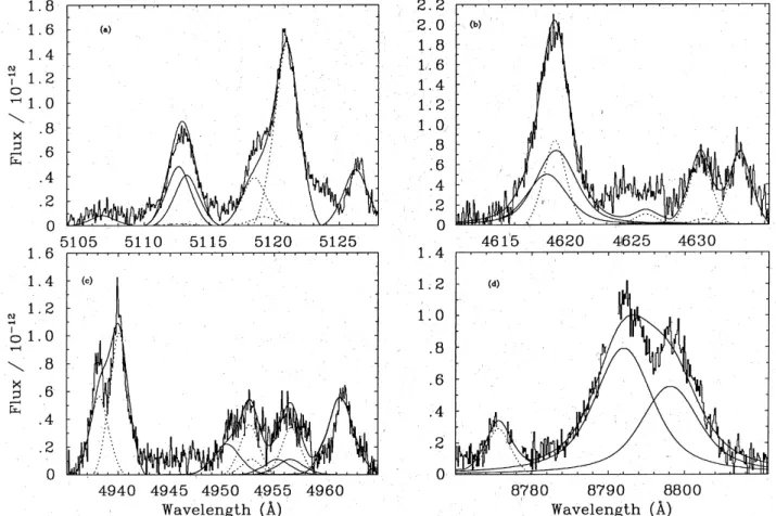
The fit to CIImultiplet 51 is shown in Figs 3(a) and 4(a).

Seven lines were identified between 5100 and 5130Å, as

shown in Table 2. The autoionizing multiplet 51 (solid line) is composed of three components, accompanied by one line of CIImultiplet 16.06 and three further lines of CIIarising from the transition array 3dp2

Po

–4fp4

D. These lines, forbid-den by LS-coupling selection rules, were iforbid-dentified when carrying out the intermediate-coupling calculations men-tioned in Section 4. There is one further unidentified line whose position and intensity were left unconstrained in the fit (component 8).

Multiplet 12 of CII is also present in this wavelength region, but its inclusion did not return a satisfactory fit and it was not retained.

5.2 CIImultiplet 50, k4619

Nine lines were recognized in the region around multiplet 50, of which eight were identified (Figs 3b and 4b, Table 3). Again, in addition to the three optically allowed 4fp2_G–3dp 2_Fo _{lines, three further 4fp} 4_G–3dp 2_Fo _{intercombination}

transitions were present, with relative intensities as given in Table 3. A systematic search for lines from high states of CII indicates, however, that the l4619 feature is also blended with the 8f–4d transition. The energy of the 8f state is not known experimentally, but can be estimated using the known positions of the 4f, 5f, 6f and 7f states. Our technique for making this estimate is described in Appendix A. The air wavelength of the 8f–4d transition is calculated to be 4620.7Å, and it is therefore completely blended with the dielectronic features of interest. An estimate of the con-tribution to the l4619 feature from the 8f–4d transition can

be made by comparison with the apparently unblended CII

8g–4f transition at l4802. We assume that the departures

from LTE for the 8g and 8f states are the same. This should be a good approximation, since heavy-particle collisions can be expected to equalize departure coefficients for states of the same n but different l. Using hydrogenic transition prob-abilities for the two transitions (Storey & Hummer 1991), we obtain a relation between the intensities which is

I(l4620.7)\1.03 I(l4802). The dereddened flux for the l4802 transition is 5.60Å10Ð12 _{erg s}Ð1 _cmÐ2 _for

CPDÐ56° 8032, and 2.48Å10Ð12_{erg s}Ð1_cmÐ2 _{for He 2–}

113. We finally make a least-squares fit to the l4619 feature, including a line of fixed intensity and corresponding to the expected flux of the 8f–4d transition. However, a good fit could not be obtained with this predicted intensity and, as can be seen from Table 3 (row 7), the fluxes for the line at

4620.7Ådiffer by about 30 per cent from their predicted

Figure 3. CPDÐ56° 8032: fits to four dielectronic multiplets of CII(a to d). Solid lines are used for the autoionizing lines, while dotted lines

values. For this reason, this dielectronic multiplet was given a higher uncertainty.

Another source of uncertainty in the determination of the flux of multiplet 50 l4621 is the level of the continuum. The local apparent continuum in this wavelength region (between 4622 and 4628 Å in Figs 3b and 4b) is about 20 per cent higher than what is estimated to be the correct con-tinuum level. Support for the correctness of our concon-tinuum placement, defined over a wide wavelength range, can be

gained by considering two weak OII lines, ll4602.11,

4609.42, belonging to the 4f 2_Fo_–3d2_{D multiplet. The}

theo-retical intensity ratio is 1.43, and the measured value using our overall continuum placement was 1.47. If the elevated continuum were used instead, the relative intensity ratio would be 2.35, in disagreement with theory. This phenome-non is also displayed by other WC10-11 stars such as K2–16, M4–18 and the WC12/R Cor Bor star V348 Sgr (Leuen-hagen, Hamann & Jeffery 1996). No bound–free process could be found to explain this local continuum enhance-ment. Another possible explanation would be the coinci-dence of many weak emission lines. In an effort to identify the lines responsible we found three lines (from the inter-Figure 4. He 2–113: fits to four dielectronic multiplets of CII(a to d). Solid lines are used for the autoionizing lines, while dotted lines are

used for the other components in the fit which arise from recombinations to bound states.

Table 2. Fitted parameters for the CIImultiplet 51. In this and the subsequent three tables, observed

wavelengths are not corrected for the heliocentric radial velocities of the stars: Ð59.4 km sÐ1 _for CPDÐ56° 8032 and Ð57.3 km sÐ1_{for He 2–113.}

mediate-coupling calculation described in Section 4 – rows 4 to 7 in Table 3) but, as can be seen from Figs 3 and 4(b), there is still surplus flux.

If the dielectronic lines are fitted using the template

pro-files derived from the 4802-Å line, the fit to the l4622

feature is too narrow. If, on the other hand, the template profile is convolved with a Lorentzian profile of a width corresponding to the lifetime of the lower state of the transi-tion, which is much shorter than the lifetime of the upper state and hence determines the width of the line, the fit is very good. This autoionization broadening is probably the explanation for the ‘unclear broadening mechanism’ encountered by Leuenhagen, Heber & Jeffery (1994) for the 4619-Å line in the star V348 Sgr (an R Coronae Borealis star that displays a spectrum not dissimilar to that of

CPDÐ56° 8032 and He 2–113). The line broadening

mech-anism is discussed further in Section 5.4.

In the spectrum of CPDÐ56° 8032 (Fig. 3b), the feature on the wavelength side is possibly due to SiIVmultiplet 6. In He 2–113 a second peak is visible (Fig. 4b). This has been attributed to NIIImultiplet 2 component l4638 (Leuenha-gen et al. 1996), but we argue that if that were the case, then we should be able to observe the principal lines of NII(e.g.,

ll4447, 3995, 5680) and NIII (e.g., ll4097, 4103 and

ll5324, 5350), and this is not the case. We fit the features

with lines whose wavelengths are left free, and the fitted line

centre wavelengths and intensities are tabulated in Table 3, rows 8 and 9.

5.3 CIImultiplet 25, k4965

Besides the autoionizing multiplet 25 (four components – see Figs 3c and 4c), we could identify three lines belonging to OIImultiplet 33. However, the fit to the region then fell noticeably below the data. We therefore introduced two unidentified lines, with free wavelengths and intensities (Table 4). This does not interfere with the derived dielec-tronic line fluxes, since the strongest dielecdielec-tronic line is almost unblended. The Earth rest frame wavelengths of the two free lines were found by the fit to be 4953.90 and

4958.27 Å for CPDÐ56° 8032, and 4954.65 and 4958.63 Å

for He 2–113. Here, as was the case for multiplet 50 (Sec-tion 5.2), a short region of elevated continuum (at 14946 Å in Figs 3c and 4c) remained unexplained.

5.4 CIImultiplet 18.01, k8794

CIImultiplet 18.01, in the far-red spectral region (Table 5), was affected by telluric lines which were removed before fitting (Figs 3c and 4d). Moreover, it came from a different echelle setting to the other dielectronic multiplets, and Table 3. Fitted parameters for CIImultiplet 50. The intensity of profile 7 is fixed at 1.03ÅI(4802) as

described in the text.

Table 4. Fitted parameters for CIImultiplet 25.

a

Intensities normalized to the CIIline l4964.73.

b

hence it might be affected by errors in the absolute flux calibration.

As was the case for the dielectronic multiplet 50 (Section 5.2), the 8794-Å triplet had to be fitted with a profile obtained by convolving the 4802-Å template with a Lor-entzian profile whose width corresponded to the predicted lifetime of the upper state of the transition (the lower level of this transition is bound, and its lifetime is much longer than the lifetime of any autoionizing level). The data pre-sented in Table 1 predict that the largest autoionizing line-width (210 km sÐ1) of the four dielectronic multiplets should be exhibited by this line. A comparison of the fit before and after this convolution was carried out and is displayed in Fig. 5. This figure clearly demonstrates the reality of autoio-nization broadening, and confirms the theoretical FWHM given in Table 1.

6 W I N D E L E C T R O N T E M P E R AT U R E S

As already described in Section 3, electron temperatures were derived by minimizing the difference between the ratios of measured and computed fluxes for the autoionizing lines. This minimization was carried out by calculating all the line theoretical intensities prior to iterating to minimize

x2

. The dereddened fluxes for the strongest dielectronic line in each multiplet are summarized in Table 6, along with the associated errors. Errors are estimated at 15 per cent for multiplets 51 and 25 of CPDÐ56° 8032, and 10 per cent for the less blended He 2–113. For multiplets 50 and 28.01, the uncertainty was determined to be about 30 per cent due to blending with the line at 4620.7 Å in the case of multiplet 50, and to being located in a different echelle setting in the case of multiplet 28.01.

If all the lines are used, and errors chosen based on the confidence in the fits, the derived electron temperatures are

18 900¹2400 K for CPDÐ56° 8032 and 17 000¹1300 K

for He 2–113. If only the two most optically thin lines are used (optical depths are calculated in Section 8), the wind electron temperature is 21 000¹2000 K for

CPDÐ56° 8032 and 16 400¹1600 K for He 2–113. To

cal-culate the parameters needed for the determination of the wind abundances, we will adopt an electron temperature of

20 000 K for CPDÐ56° 8032 and 17 000 K for He 2–113.

The electron temperature derived here for the wind of CPDÐ56° 8032 is higher than the value of 12 800 K derived by Barlow & Storey (1993), who used Gaussian fits to the flux in the entire multiplets in their lower resolution (0.5 Å) spectrum.

Table 5. Fitted parameters for CIImultiplet 28.01.

Figure 5. Comparison between fits to the 8794-Åmultiplet components before (a and b) and after (c and d) convolving the template profile with a Lorentzian of width corresponding to the autoionization lifetimes of the two upper states of the transition.

7 S T E L L A R W I N D A B U N D A N C E S F R O M R E C O M B I N AT I O N L I N E S

To determine the relative abundances of He+, He2+, C2+, C3+ _{and O}2+_{in the stellar winds, we used recombination}

lines from a number of multiplets belonging to these ions, assuming that the winds are optically thin to the chosen lines.

Abundances derived in this way provide a useful check on the abundances derived by bulk modelling of the stellar atmosphere (e.g. Hillier 1989; Hamann et al. 1992). More-over, the large amounts of computing time needed to con-struct models spanning a large spectral range makes direct methods all the more appealing. In the case of

CPDÐ56° 8032 and He 2–113, modelling has been carried

out by Leuenhagen et al. (1996), while in Paper II computa-tional modelling of both stars is reported and extensive comparisons with the work of Leuenhagen et al. are made. For these two stars it is possible to measure a substantial number of unblended lines of all the ions present, and hence to derive total abundances by summing the individual ionic contributions.

It is well known that the winds of WR stars have consider-able ionization stratification (e.g. Hillier 1988). However, Smith & Hummer (1988) have shown (in their section 7.4) that, even in a stratified wind, the elemental abundances are exactly given by the sum of the individual ionic emission measures, provided that the innermost radius from which the used lines are capable of emerging is the same for both species. This is usually the case if the lines used have similar wavelengths, since the innermost shell from which the line radiation is still capable of emerging is a function of the continuum opacity, which is in turn a slow function of wave-length. The other main source of opacity, the line opacity, is thoroughly discussed in Section 8.

Since effective recombination coefficients and collisional rates are temperature-dependent, the wind electron tem-peratures derived in the previous section were used to cal-culate the emission measures. The C2+ion is the dominant ion stage of carbon in the winds, and this method diagnoses

the temperature in the C2+ _{line formation region. We}

assumed that the OII and CII lines originate in similar

regions, together with the HeIlines (although O2+, with a higher ionization potential than C2+, might extend deeper into the wind, where the electron temperature is higher). We will also discuss the use of the CIIdielectronic lines as abundance diagnostics, along with the CIIradiative recom-bination lines.

The abundance of an ionic species is determined from

equation (5), where the expression for Q for the dielectronic lines can be found in equation (6), while for ordinary bound–bound recombination lines we obtain

Q(l, Te)\hvaeff. (9)

Integrating over the volume of emission,

I Q\

1

4pD2[Ni], (10)

where [Ni] represents the product of the ionic and electron densities integrated over the emitting volume. The ratio of the emission measures of two ionic species can thus be obtained in a straightforward manner:

[Ni] [Nj]

\Ii/Qi

Ij/Qj

. (11)

To obtain the relative abundances for a pair of elements, one takes the ratio of the total emission measure for each of the elements, after summing over all the observed ioniza-tion stages. Thus for elements X and Y, with number densi-ties NXand NY, NX NY Ðdp[N +p X ] dq[N +q Y ] . (12) In the case of He0

transitions, allowance had to be made for collisional population of the upper levels from the 23_S

metastable state. For the HeIlines at 4471.5, 5875.7, 7065.3 and 6678.1 Å, the collisional rates needed to calculate the rate of collisional to radiative recombination population (C/

R), were obtained from Kingdon & Ferland (1995). In the

Kingdon & Ferland expression for C/R, the total HeI

recombination coefficient and the line effective recombina-tion coefficient are calculated for a low (1106_cmÐ3₎

elec-tron density. However, since such coefficients appear in both the numerator and denominator, the effect of density cancels out to a first approximation. We used the collisional excitation formulation of Clegg (1987) for the HeIlines at 4713.2 and 5047.7 Å. We updated Clegg’s formulae with new values for the effective recombination coefficients of the two lines, obtained by one of us (PJS), and new colli-sional excitation rates from Sawey & Berrington (1993). A

density of 1011 _cmÐ3 _{and temperatures of 20 000 and}

17 000 K were used for CPDÐ56° 8032 and He 2–113

respectively (for the 17 000-K case we interpolated between the tabulated values).

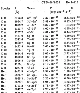
Table 6. Summary of the dereddened fluxes measured for the strongest

compo-nent of each dielectronic multiplet for CPDÐ56° 8032 and He 2–113, together with associated error estimates.

High-density (1011

cmÐ3) recombination coefficients were also available (Davey 1995) for the CIIlines at 4493 Å2(9g– 4f), 4802 Å (8g–4f), 5340 Å (7g–4f) and 6461 Å (6g–4f), which were observed unblended in the spectra of both stars. For the CIIline at 4267 Å, high-density effective recombi-nation coefficients were also obtained from Davey, although they were tabulated only for a temperature of 12 800 K. To scale them to the right temperatures, scaling factors of 1.56

(CPDÐ56° 8032) and 1.32 (He 2–113) were calculated by

comparing hydrogenic effective recombination coefficients (Storey & Hummer 1995) for a density of 1011_cmÐ3_{and for}

temperatures of 12 800, 20 000 and 17 000 K.

For the C3+_{ion, hydrogenic recombination coefficients}

from Storey & Hummer (1995) were also used. The CIII

lines used for the abundance determination originated from high transitions, and the hydrogenic approximation was considered to provide sufficient accuracy.

For the He2+_{ion, only the 4–3 l4686 line was used, and}

its recombination coefficient was taken from Storey & Hummer (1995).

For the OII ion, new OIIrecombination coefficients at low electron densities have been tabulated by Liu et al. (1995). These new intermediate-coupling recombination coefficients are expected to be more accurate than any cur-rently in the literature. Case B was assumed to prevail, in the sense that all radiative transitions to the ground term 2s2

2p3 4

So

are assumed to be optically thick. This assumption was found by Liu et al. to be necessary to obtain agreement between the O2+abundances derived from different multip-lets in the nebular spectrum of NGC 7009. In particular, the

3d–3p transition gives O2+abundances which differ by an

order of magnitude from the others, if case B is not assumed. These recombination coefficients were calculated for a density of 106

cmÐ3and not for a density of 1011

cmÐ3, more appropriate to the WC10 wind emission regions. For higher densities, the recombination coefficient increases,

making the I/Q ratios smaller and hence the derived O2+

abundances lower. For this reason we consider our O/He abundance ratios of 0.35 for both objects, to be upper limits. However, to give an indication of the effect of a higher electron density, a scaling factor was calculated by compar-ing the effective recombination coefficients for low (104

cmÐ3) and high (101_cmÐ3_{) density for C}

IItransitions with the same configuration as the OIItransitions used (3d–3p

and 4f–3d). Recombination coefficients for C2+were

cal-culated at 12 800 K by Davey (1995) for densities of 104

and 1011_cmÐ3_{. Applying these facors (1.45 for the 3d–3p}

trnsi-tion and 1.34 for the 4f–3d transitrnsi-tion), the derived O/He

ratio becomes 0.24 for CPDÐ56° 8032 and 0.25 for He 2–

113.

The observed stellar wind emission-line fluxes are pre-sented in Table 7, while the dereddened line fluxes are listed in Table 8. The errors associated with the flux measure-ments were about 10 per cent for the CIIIlines (although for the weaker 9g–4f lines at 4493 Å they might have been slightly higher) and about 15 per cent for the weaker OII and CIIIlines. The HeIlines, despite being stronger and easier to measure, always had P Cygni profiles, so that the

red side had to be projected on to the blue side about the centre of the line, with the uncertainties involved gauged at about 20 per cent. We estimate an uncertainty of 10 per cent for the flux of the HeIIl4686 line.

In selecting the OIIlines to use as diagnostics, we looked for unblended lines or blends whose components belonged to the same multiplet. Beside the lines listed in Table 7 (for which a detailed description follows) we found three other candidates, multiplet 53.03 at 4237.93 Å, multiplet 26 at 4395.97 Å and multiplet 33 at 4941.09 and 4943.02 Å. For all of these, however, the I/Q ratios were one order of magnitude higher than for the OIImultiplets groups listed in Tables 7 and 8. We therefore decided to disregard them on the grounds that if the I/Q ratio for a line is too high, it can mean that its flux was overestimated due, for instance, to blending.

We finally used three OII multiplets. Multiplet 28 has three components (4890.8, 4906.8 and 4924.5 Å). Two of these were measured, and their fluxes are given in Table 7. Multiplet 20 contains seven components, some of which are

blended together. For CPDÐ56° 8032, we measured the

flux corresponding to the blend of ll4103.0, 4105.0 and

4104.7 (three of the seven components of multiplet 20),

while for He 2–113 the weak l4103.0 component was

resolved and was not included in the measurement. These multiplet 20 fluxes are tabulated in Table 7, in the row corresponding to OII4105 Å. What is tabulated as l4277.0 in Table 7 is, in fact, the sum of the four components of OII multiplet 67.

Four of the nine CIIlines that were used are the dielec-tronic lines used in the wind electron temperature determi-nation. The remaining five lines form as a result of the ng–4f

2

The energies of the nf and ng series are known experimentally up to n\7 (f series) and n\8 (g series). See Appendix A for the energies of the higher members of these series.

Table 7. Stellar emission-line fluxes for CPDÐ56° 8032 and

He 2–113 (before dereddening). For the HeIlines, singlet (S)

(n\6 to 9) transitions already discussed, plus the 4f–3d 4267-Å transition. This line is usually thought to be much more optically thick, and not to be suitable for abundance determinations. However, we believe this not to be neces-sarily the case, and we introduce it here; its optical depth will be analysed in Section 8.

CIIIlines were chosen with upper levels as high above the ground state as possible and with orbital quantum numbers as large as possible, so as to make the hydrogenic approxi-mation, used in deriving the effective recombination coeffi-cients, as realistic as possible. We chose the lines at 5303.1 Å (multiplet 46, 5f3

Fo

–7g3

G) and at 8665.2 and 8663.6 Å (multiplet 45, 6g3_G–5f3_Fo_{). The measurement was}

slightly more difficult in the case of He 2–113 than for

CPDÐ56° 8032, due to the l8665.2, 8663.6 lines being

blended with the nebular hydrogen Paschen series line

(n\14–3, 8665.02 Å), while the l5303.1 line had a mild

P Cygni profile. Despite the difficulties encountered, it can be seen from Table 8 that the I/Q values derived from the two lines are in agreement. An error of 30 per cent is quoted, which includes a 15 per cent uncertainty in the line flux measurements, and a 15 per cent uncertainty in the effective recombination coefficients. In conclusion, for both

objects the C3+ _{abundance is found to be more than 500}

times smaller than the C2+abundance.

After the HeI lines had been corrected for collisional effects, the corrected fluxes were used to obain the emission measures listed in Table 8, as described by equations (9) and (10). The I/Q values for all the ions were then averaged using the weights for each line listed in columns 7 and 11 of Table 8. The weights are based on the confidence in the I/Q ratio, once all the sources of uncertainty were taken into consideration. The averaged I/Q values of different ioniza-tion stages of the same element were then summed, with the summed I/Q values from the carbon, oxygen and helium ions yielding the final abundance ratios listed in Table 9. The weights given to the I/Q values in Table 8 are based purely on the measurement uncertainty, and do not take into account optical depth effects.

In Table 10 we compare the stellar wind abundance results derived from our recombination line analysis with those of Leuenhagen et al. (1996), who constructed non-LTE models for these and other [WCL] stars, and with our own non-LTE wind modelling (Paper II). We find values of C/He comparable within the uncertainties, while our O/He ratios are higher than the values obtained by Leuenhagen et al., but comparable, within the uncertainties, with the values derived in Paper II.

Contrary to Leuenhagen et al. (1996), we find that both stars have no detectable hydrogen in their winds (see Papers Table 8. Dereddened fluxes and I/Q values determined for unblended stellar features. Most of the OIIlines were blends of

several components. Details of which components were used are given in the text. C/R correction factors are given for the HeI

I and II). This restores these [WCL] stars to their former status as hydrogen-free WR stars.

8 O P T I C A L D E P T H E F F E C T S

In the abundance determinations in Section 7 we have made use of lines between low-lying states of He, O and C which might reasonably be expected to have different and not insignificant optical depths. In addition, the wind tempera-ture determinations have tacitly assumed that the dielec-tronic lines are optically thin. In this section we discuss the effect of line optical depth on our conclusions.

The optical thickness of the wind in a given transition depends, inter alia, upon the population of the lower state of the transition and the oscillator strength for that transition. For a series of transitions terminating in a common lower state, the oscillator strength falls as nÐ3, where n is the principal quantum number of the upper state, while the population of the lower state decreases as its energy increases. The decline in optical thickness with increasing upper state principal quantum number is illustrated by the

ng–4f series in CII(6RnR9) which are visible in our spec-tra. These lines, which display no P Cygni structure, show a decreasing FWHM as n increases (see Table 12). This effect, which has also been described in Population I WR stars by Schulte-Ladbeck et al. (1995), is attributable to the decline in optical thickness, since the emission from the inner, low-velocity part of the wind is relatively stronger for less optically thick lines, while the emission from the outer higher velocity part is approximately unchanged, leading to

an apparent narrowing of the line. On the basis of the empirical evidence from line FWHM, the winds of the two stars are optically thick to many of the lines used in the abundance analysis. None the less, the abundances derived from the various lines of apparently different optical depths are in broad agreement, although there is a tendency for the abundances derived from the dielectronic lines to be lower

than from the CII bound–bound transitions. The optical

thickness of the CII dielectronic lines cannot be assessed empirically from their FWHM due to blending and the additional autoionization broadening that some of the lines exhibit. They certainly arise from energetically high-lying atomic states but, being 3p–3d and 3d–4f transitions, they have relatively large oscillator strengths. In addition, the wind models described in Paper II do not include the tem-perature diagnostic dielectronic lines, so we have carried out an escape-probability analysis of these and other lines to determine their optical thickness.

Table 9. Elemental abundance ratios, by number, for the

winds of CPDÐ56° 8032 and He 2–113.

Table 10. Comparison of abundances (by

number) for CPDÐ56° 8032 and He 2–113 derived here using exclusively recombination lines from bound–bound transitions, with abun-dances derived by bulk non-LTE modelling of the stellar atmosphere (Paper II) and the non-LTE study of Leuenhagen et al. (1996; LHJ).

We use the escape-probability formalism of Castor (1970) for an expanding spherically symmetric atmosphere, in which an optical depth t(z, r) is defined by

t(z, r)\pe 2 mcÅ(gf )u,lÅ (Nl/glÐNu/gu)År vovr/c Å 1 1+z2_/r2_{(d ln v/d ln rÐ1)} , (13)

where r is the distance from the centre of the star, z is the distance from the centre of the star projected in the direc-tion to the observer, f is the oscillator strength for the level,

vois the frequency at the line centre, and the velocity field

has the (assumed) form

v(r)\vl

2

Rc

r

3

g

, (14)

where v_lis the terminal velocity of the wind, Rcis the radius

of the star (defined from the centre to the base of the wind), and g, which defines the degree of acceleration of the wind, is usually taken to be 1. With this velocity law, the logarith-mic derivative of v with respect to r is Rcvl/rv(r).

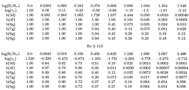
We take the physical quantities needed to define the model from the results of Paper II. For each star a grid was established of 10 points that spanned the depth of the wind. Grid points were equally spaced in log(tRoss) (where tRossis

the Rosseland optical depth). For each grid point we extracted the physical radius, the electron temperature and density, the fraction of C2+_{and He}+_{(see fig. 4 in Paper II),}

the continuum optical depth (at 5000Å) and the departure coefficients for the upper and lower levels of each transition (see Table 11). These last two quantities were obtained from the models described in Paper II, but are not explicitly given there. For the dielectronic transitions we calculated b-values from equation (2) and Table 1 for states above the ionization limit, while for lower levels the b-values were set to unity. The wind model of Paper II did not include the 9g level – its departure coefficients were set to the same values as the 8g level.

In the model, we neglect the stellar continuum and its absorption by the lines, obtaining the flux emitted in the lines as a function of radius and of velocity. We obtain

predicted relative fluxes for all the dielectronic lines of CII

and for the bound–bound transitions of CII and neutral

helium. The optical depth in the lines can also be monitored throughout the wind.

8.1 Results of the escape-probability model

In Table 12 we present a summary of the predicted fluxes (on an arbitrary scale) for a sample of lines, their calculated optical depths and their observed FWHMs. The optical depths are calculated at a point with z\0 at a radius corre-sponding to the peak of the line formation region, which

was determined to be 3.0R_* for CPDÐ56° 8032 and 2.5R_*

for He 2–113. We use the tabulated optical depth values only for comparison purposes.

We observe, first of all, that the trend in optical depths of the bound–bound lines confirms the trends outlined above, that the more optically thick lines come from lower levels, and that the optical depth falls when progressing up a series with a common lower state (4f–6g, l6450; 4f–7g, l5340; 4f– 8g l4802). Also, the relative fluxes from the model (Table 12) agree reasonably well with the observed relative fluxes (Table 12 and 8), for both bound–bound and dielectronic lines, suggesting that the low I/Q values obtained from the dielectronic lines are due to the effects of opacity and their particular atomic physics (see Section 8.2 below), rather than to uncertain measurements. Table 12 also confirms that some lines between low-lying states (e.g., l4267 4f–3d of CIIor the l5876 triplet of HeI) which give reasonable abundances have very high optical depths. It appears that the line fluxes predicted by the theory of recombination in an optically thin medium also approximately describe the emission from lines of high optical thickness, with the exception of the dielectronic lines, where relatively modest optical depths significantly affect the derived abundances. In the next section we seek to explain these observations.

8.2 A two-level atom

Consider a two-level atom in which the populations are determined solely by radiative processes, both bound–free and bound–bound (although we will neglect photoioniza-tion). The population of the upper level (N2) is given by

NeN+a2\N2G R

21b21, (15)

Table 11. Continuum opacities (tc) and departure coefficients for all the levels used, as a function of log (R/R *). The stellar radius for CPDÐ56° 8032 was 2.0 R>, while for He 2–113 it was 2.5 R>.

Table 12. Predicted normalized fluxes compared with

observa-tions, optical depths and observed FWHM for a sample of CIIand

HeI lines used in the derivation of abundances (T stands for

triplet).

†rp\3.0R

* for CPDÐ56° 8032. †rp\2.5R

where GR

21is an Einstein A-coefficient, a2is a recombination

coefficient, and b21is the single-flight escape probability for

photons in the transition, which decreases as the optical depth increases. The emissivity in the transition is just

N2G R

21b21hv\NeN+a2hv, which is the same as in the optically

thin case, no matter how great the optical depth in the line. As the optical depth increases, the population of the upper state rises so that the flux in the line is preserved. The abundance derived from such a transition using optically thin recombination theory will be independent of optical depth.

Consider now an ideal dielectronic line where the two states are embedded in the continuum, their populations are given by the Saha equation and are independent of the optical depth. The emissivity N2G

R

21b21hv will fall as the

opti-cal depth increases due to the fall in the escape probability, and the abundance derived from the transition will fall as the optical depth rises.

In practice, all states are coupled to each other and the continuum by collisional processes, so the purely radiative

case described above is never realized in practice, but the

l4267 4f–3d transition in CII might be expected to be a reasonable approximation. Both states are low-lying, so that collisional processes are relatively unimportant and, as in the model two-level atom, there is no alternative decay route from the 4f state once the transition becomes optically thick.

To illustrate these effects for a transition uhl, we define an effective recombination coefficient apulby

NeN+apul\NuG R

ulbulhv, (16)

so that ap is a measure of the emissivity in a particular transition allowing for the effects of optical depth. In Fig. 6 we show the behaviour of this quantity as a function of radius in the wind of CPDÐ56° 8032. In each plot, the horizontal line segment shows the value of the effective recombination coefficient for that particular transition, taken from optically thin recombination theory at the tem-perature of maximum emission in the wind. The length of the segment represents the width of the line-forming region,

Figure 6. Effective recombination coefficients in the optically thin case (line segments), allowing for optical depth effects as defined in

equation (16) (curves) for selected lines of CIIand HeI. The vertical lines mark the peak of the emission region for the line, while the width

of the horizontal segments approximately shows the FWHM of the emission region. Both for HeIlines and for the CIIline at 4267 Å the emission region extends further towards the surface of the star than for the CIIlines in the ng–4f series or the dielectronic lines at 4619, 4965

as indicated by fig. 4(e) in Paper II. These are the values that were used to determine the abundances in Table 8. The vertical line shows the approximate radius of maximum emission in the recombination lines. This is taken to be at 3R

* for the peak of the CIIline-forming region, and at 5R* for the peak of the HeIline-forming region. We note that the values of ap at the radius of maximum emission generally lie within about a factor of 3 of the optically thin theory, even though the optical depths in the lines range from about 0.5 to 241. We note also that the values of ap for the three dielectronic lines ll4619, 4965, 5114 are all smaller than the corresponding optically thin values, as expected.

We have not included the recombination lines of OIIin this analysis, but some general points can be made by com-paring OIIwith CII. Due to the 3P parentage of the OII configurations, a particular valence electron configuration of OIIresults in many more states than the corresponding CIIconfiguration. For example, the two OIIlines of multip-let 28 listed in Table 8 correspond to transitions to the 3p(4

So

3/2) state. This state, with a statistical weight of 4, will

have a population approximately 4/54 of the whole (3

P)3p configuration. If all other factors were equal (elemental abundance, distribution in the wind, oscillator strengths and energies of states), the optical depth of the OIIlines would be lower than that of the corresponding CIItransitions by

the same factor. We conclude the OII lines used in the

abundance analysis are likely to have low optical depths and be correspondingly more reliable as abundance indicators, although other problems with these lines have been dis-cussed above.

We would like to underline that the above arguments are only qualitative in nature. Only a complete modelling of the whole envelope can give us any assurance of a correct treat-ment of the opacity. However, from this limited exercise we conclude that low-lying bound–bound transitions can be combined with optically thin recombination theory to obtain indicative abundances. As a result, we prefer to use bound–bound rather than dielectronic transitions for our abundance determination.

As far as the wind electron temperature is concerned, we see from Fig. 7 that the escape probabilities for the ll5114,

4965 lines are very similar throughout the wind (while the escape probability for the CIIl4619 line is much lower), implying that the two lines will be equally attenuated by the wind and their ratio therefore preserved. This gives renewed confidence in using these first two lines to deter-mine the wind electron temperature.

9 S U M M A RY

We have demonstrated the use of low-temperature dielec-tronic recombination lines for the determination of the wind electron temperature of [WC10] central stars of PNe. For CPDÐ56° 8032 we obtain 21 700¹2000 K, while for

He 2–113 we determined 16 400¹1600 K. This is the first

direct spectroscopic determination of such a quantity in a WR star. Stellar wind abundances have also been derived for carbon and oxygen relative to helium. We derived C/ He\0.44 and 0.29 for CPDÐ56° 8032 and He 2–113 respectively, while for oxygen, an upper limit of O/He\0.35 was obtained for both stars and, after correcting recombina-tion coefficients for the high density of the wind, values of

0.24 and 0.26 were obtained for CPDÐ56° 8032 and He 2–

113 respectively. The oxygen lines used all arise from bound–bound transitions. Moreover, the opacity of such lines is lower, due to the different atomic structure of the

OII ion. Carbon abundances are derived using bound–

bound transitions, not the dielectronic recombination lines, since these systematically underestimate the abundance due to optical depth effects. This is due to their upper levels being in LTE with the continuum and not being able to compensate for optical depth by increasing their upper level populations.

Optical depth effects are not thought to influence the electron temperature determination, since the escape prob-abilities of the two most optically thin dielectronic lines are almost identical throughout the wind.

A C K N O W L E D G M E N T S

OD acknowledges the Perren Fund for providing support during the completion of her PhD.

A P P E N D I X A : T H E E N E R G I E S O F T H E 2 s2_{n f A N D 2 s}2_{n g S TAT E S O F C}+++

For the 2s2

nf series of C+, energies are measured for nR7,

while for the 2s2

ng series measurements exist up to n\8

(Moore 1970). The quantum defect m is defined by

Inl\

ÐZ2

RC

(nÐm2₎ , (A1)

where Inlis the ionization potential of state with principal

quantum number n and orbital quantum number l, Z is the

effective charge (Z\2 for C+_{), and}

RC\

Rl

1+me/Amu

is the Rydberg constant for carbon, where R_l\109 737.3,

me is the electron mass, mu is the atomic mass unit, and

A\12 is the atomic mass number.

For a one-channel problem, the quantum defect is related to the reactance matrix of quantum defect theory by (Seaton 1983),

R\tan(pm). (A2)

The reactance matrix for the 2s2

nf2

Fo

series has poles at the energies of the C+2s2p(3_Po_{)nd states. Considering only the}

lowest of these poles, we fit the reactance matrix to a

func-tion of the energy variable e\Ð1/(nÐm)2

,

R\a+be+ c

(eÐe0)

, (A3)

where e0\0.007 52 corresponds to the position of the

3dp(2_Fo

) state. Values of R and hence m can then be obtained for higher members of the 2s2

nf series. The

result-ing energies are given in Table A1 relative to the ground state of C+.

For the 2s2

ng series a different procedure is used. The

quantum defects for this series can only be perturbed by states of the 2s2p(3

Po

)nf series, whose lowest member n\4 lies at sufficiently high energy that this effect can be neg-lected. We therefore analyse the quantum defects of the 2s2_{ng states in terms of the dipole polarizability, a}

d. The

quantum defect can be expressed in terms of the polariz-ability by ad\ 2m Z2 n3 P(nl) , (A4) where P(nl)\ (3n 2_Ðl2_Ðl) 2n5_(lÐ1 2)l(l+ 1 2)(l+1)(l+ 3 2) . (A5)

From the experimental energies for the 5g and 6g states

we deduce ad\3.9. Term energies for the higher members

of the ng series can then be inferred from the above two equations, and the results are given in Table A1.

Table A1. Energies for states 2s2

nf and 2s2 ng deduced by quantum defect extrapolation.

R EFER ENCES

Barlow M. J., Storey P. J., 1993, in Weinberger R., Acker A., eds, Proc. IAU Symp. 155, Planetary Nebulae. Kluwer, Dordrecht, p. 92

Bidelman W. P., MacConnell D. J., Bond H. E., 1968, IAU Circ. 2089

Castor J. I., 1970, MNRAS, 149, 111 Clegg R. E. S., 1987, MNRAS, 229, 31

Crowther P. A., De Marco O., Barlow M. J., 1998, 296, 367 Davey A. R., 1995, PhD thesis, Univ. London

De Marco O., Crowther P. A., 1998, MNRAS, 296, 419 (Paper II)

De Marco O., Barlow M. J., Storey P. J., 1997, MNRAS, 292, 86 (Paper I)

Eissner W., Jones M., Nussbaumer H., 1974, Computer Phys. Com-mun., 8, 270

Hamann W.-R., Leuenhagen U., Koesterke L., Wessolowski U., 1992, A&A, 255, 200

Henize K. G., 1967, ApJS, 14, 125 Hillier D. J., 1988, ApJ, 327, 822 Hillier D. J., 1989, ApJ, 347, 392

Howarth I. D., Murray J., 1991, PPARC Starlink User Note No. 50.13

Kingdon J. B., Ferland G. J., 1995, ApJ, 442, 741 Leuenhagen U., Hamann W.-R., 1994, A&A, 283, 567 Leuenhagen U., Heber U., Jeffery C. S., 1994, A&AS, 103, 445 Leuenhagen U., Hamann W.-R., Jeffery C. S., 1996, A&A, 312,

167

Liu X.-W., Storey P. J., Barlow M. J., Clegg R. E. S., 1995, MNRAS, 272, 369

Martin W. C., Kaufman V., Musgrove A., 1993, J. Phys. Chem. Ref. Data, 22, No. 5, 1179

Moore C. E., 1970, Selected Tables of Atomic Spectra, Nat. Stan. Ref. Data Ser. Nat. Bur. Stand. (U.S.), 3, Sec. 3

Nussbaumer H., Storey P. J., 1978, A&A, 64, 139 Nussbaumer H., Storey P. J., 1983, A&AS, 56, 293

Sawey P. M. J., Berrington K. A., 1993, Atomic Data and Nuclear Data Tables, 55, 81

Schulte-Ladbeck R. E., Eenes P. R. J., Davis K., 1995, ApJ, 454, 917

Seaton M. J., 1983, Rep. Prog. Phys., 46, 167 Smith L. F., Hummer D. G., 1988, MNRAS, 230, 511 Storey P. J., 1981, MNRAS, 195, 27

Storey P. J., Hummer D. G., 1991, Computer Phys. Commun., 66, 129

Storey P. J., Hummer D. G., 1995, MNRAS, 272, 41

van der Hucht K. A., Conti P. S., Lundstrom I., Stenholm B., 1981, Space Sci. Rev., 28, 227