Aerodynamic Optimization of a Solar Powered Race Vehicle
by
Peteris K. Augenbergs
Submitted to the Department of Mechanical Engineering in Partial Fulfillment of the Requirements for the Degree of
Bachelor of Science
at the
Massachusetts Institute of Technology December 2005
C 2005 Peteris K. Augenbergs All rights reserved
The author hereby grants to MIT permission to reproduce and to distribute publicly paper and electronic copies of this thesis document in whole or in part in any medium now
known or hereafter created.
Signature
of Author...
...
...
Department of Mechanical Engineering December 14, 2005
Certified by
...
...i
J. Kim VandiverDean for Undergraduate Research
Accepted by ... ...
John H. Lienhard V Chairman of the Undergraduate Thesis Committee
Aerodynamic Optimization of a Solar Powered Race Vehicle by
Peteris K. Augenbergs
Submitted to the Department of Mechanical Engineering on December 14, 2005 in Partial Fulfillment of the Requirements for the Degree of Bachelor of Science
ABSTRACT
Aerodynamic optimization was performed on Tesseract, the MIT Solar Electric Vehicle Team's 2003-2005 solar car using Wind Tunnel 8 at Jacobs/Sverdrup Drivability Test Facility in Allen Park, MI. These tests include angle of attack and ride height
optimization, as well as vehicle-level details such as wheel fairing length, surface finish, sealing, and rear-view mirrors. These tests achieved a net reduction in drag, an increase in stability due to lift force reduction, and valuable knowledge of boundary layer conditions which will be used in future designs.
Thesis Supervisor: J. Kim Vandiver Title: Dean for Undergraduate Research
Introduction
Aerodynamic drag is the single largest power sink on a solar car, accounting for approximately 70% of the total power consumption. This necessitates significant effort in the aerodynamic design and optimization of a solar car. The 2005 North American Solar Challenge is the longest solar car race in the world, spanning 2500 miles on public roads from Austin, TX to Calgary, AB. In order to be competitive with the best in the field, every single system of the car must be optimized for efficiency. This paper outlines the aerodynamic optimization techniques we used on Tesseract, the MIT entry to the North American Solar Challenge.
Background
The rules for the North American Solar Challenge allow maximum dimensions for single seat solar cars of 1.8 by 5 meters in plan view, with a maximum height of 1.6 meters. Other design constraints laid out by the rules are a minimum eye height of 70
centimeters, 100 degrees of vision to either side in the front, and 30 degrees to either side in back. The rules also specify that the vehicles must have a minimum of 3 wheels in contact with the ground at all times. These rules give a rough shape for a solar car, within which the teams have unlimited freedom for aerodynamic design and
optimization.
Given the maximum planview area of 9 square meters, this allows about 9 kilowatts (KW) of energy at solar noon in good conditions available to work with. The
photovoltaic cells on the market range from 10%-30% in efficiency. Amorphous silicon terrestrial grade cells are on the low end, and the best multi-junction Gallium Arsenide space grade cells are on the high end. The top solar car teams use space-grade cells that
have slight defects, which gives them an efficiency of 20-25%. The MIT Solar Electric Vehicle Team (SEVT) was able to obtain a lot of triple-junction cells with an average efficiency of 25.5%. This puts an upper bound on power available at noon of 2.3 KW.
With so little power available, and the goal to maximize average race speed, it becomes necessary to develop a model for power consumption of an efficient electric vehicle, and to create a power budget to choose what is most important to optimize. The 5 things that consume power on the car are rolling resistance, aerodynamic drag, electrical/motor efficiency, acceleration, and hill climbing. The power required for each of these can be derived from basic physics, or some empirical measurements and calculations.
PTotal = Peo + PIoing + Pccration + Phills (1)
F= Fv
(2)
Using Equation 2 with the defined forces for aerodynamic drag, rolling resistance, and acceleration: 1 Per = CdA pv (3) 2 P ,oiing = C,,mgv (4) Paceeratio = vma (5)
P,, = mgvd
(6)
Using the defined efficiency from electrical energy to mechanical energy for the motor and controller,
Plectrical - (7)
7lmotor
Substituting Equations 3 through 7 into Equation 1,
plVctr(cal=
pV
2CdA+ m(
C,g+
a+gdh
(8)
]?motorWhere P is power in Watts, F is force in Newtons, v is the car velocity in meters per second,, p is the density of the fluid in kilograms per cubic meter, g is the acceleration due to gravity, a is the car's acceleration along the road, and dh/dx is the grade of the road.
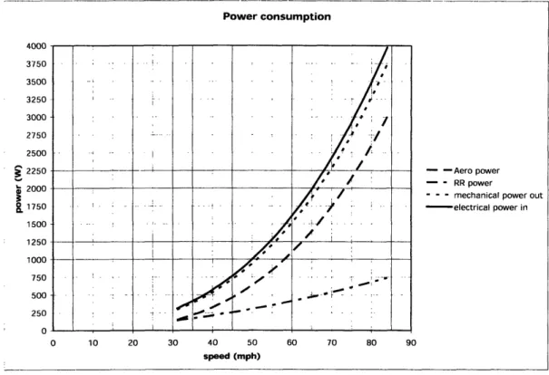
The values for these coefficients and quantities for the 2003 MIT solar car can be found it Table 1. A plot of each power versus velocity, as well as the total electrical power versus velocity quickly shows that aerodynamic drag accounts for about 70% of the power consumption of a typical high-performance solar car at highway speeds. See Figure 1.
Power consumption 3750 3500 3250 3000 2750 2500 j 2250 ° 1750 1500 1250 1000 750 500 250 0 - - Aero power - - RR power
- - - mechanical power out
electrical power in
0 10 20 30 40 50 60 70 80 90
speed (mph)
Figure 1. Power consumption of aerodynamic drag, rolling resistance, and motor losses, and total power as a function of vehicle speed.
With aerodynamic drag consuming the majority of the vehicle's power, it quickly becomes apparent that it is the single most important system of the car to optimize. For
streamlined bodies like a solar car, the drag coefficient best scales with wetted area instead of the automotive industry standard frontal area. (Tamai 11) The trick here is that with a thin, flat car like most solar cars, the solar power available scales with the planview area, which is approximately half the wetted area. Assuming that CdA and
solar power both scale linearly with planview area, using the solar array efficiency and Equation 3, the solar power increases about 210 W/sq. m., at the cost of about 136 W in aerodynamic drag at 60 mph. This sets the optimum array size at the max dimensions prescribed by the rules.
Given budget constraints at the beginning of the 2005 project, the MIT SEVT chose to reuse the main body and solar array from the 2003 car that finished 3rd in the World Solar
Challenge in Australia. These budget constraints prevented the team from modifying the foil shape for the main body, but allowed wheel fairing redesign, and optimization of the ride height, and angle of attack. The body was designed with a neutral angle of attack and 30 cm ride height, but the design was only verified with two-dimensional computational fluid dynamics using XFOIL and AIRSET. This design validation neglected the variance from the centerline foil across the section of the car, as well as the flow due to the wheels and wheel fairings.
The primary goal of this study was primarily to optimize the aerodynamic lift and drag performance using full-scale wind tunnel techniques at the Jacobs/Sverdrup Drivability Test Facility Wind Tunnel 8 in Allen Park, MI. This optimization study was to directly benefit the MIT SEVT's performance in the North American Solar Challenge in July 2005. The secondary goal was a design validation to learn if the car was performing as designed and if not, to determine the underlying cause. This information will be used directly in designing the next MIT solar car.
Methods
Ford Motor Company graciously donated two 8-hour shifts of wind tunnel time at DTF WT8. In the process of developing a test plan for the two shifts, I consulted with Mark Drela in the Aero/Astro department and Goro Tamai, an alumnus of SEVT. The
designed test plan was dynamic; future tests were based on results of previous tests. The tests with the largest co-dependence were divided between day 1 and day 2, which
allowed for more thorough analysis and also for the construction of mockups for testing on day 2. The final test matrix is in Appendix A.
The car was installed on the load cell pads and the suspension was strapped down to hold the vehicle in place. Because of our 3-wheel design, the folks at Sverdrup made a spreader bar to distribute the load of the center rear wheel to the two rear load cell pads. After the chassis was fixed to the test platform, we attached the solar array and measured the distance to the tunnel floor at the nose, center, and tail of the car. From this, we could back out the angle of attack of the body, as well as the ride height. To adjust parameters like angle of attack and ride height, I machined some chassis spacers to replace the coil-over shocks on the car. By creating a set of bars with various center-to-center distances between eyes, we could precisely control the car's attitude and height from the wind tunnel floor. After optimization, these parameters could be controlled with suspension preload or even ballast if necessary to ensure optimal aerodynamic performance.
After the initial setup, we performed a shakedown run at 70 mph at max yaw to ensure the car was secure and stable in the tunnel. On the first try, one of the straps holding down a front wheel came loose, and the wheel actually lifted off the ground several
inches, necessitating an emergency stop of the tunnel. For each test configuration, we set the car up like we wanted, and then went back to the control room and specified the speed and yaw angles we wanted for that particular setup. It took about a minute per data point to get the measurements to converge, so each test setup, signified by a row in the test
The data we received from Sverdrup is divided into runs, which equate to test setups from our actual test plan. Most are yaw sweeps, while others are single points or sets of speed tests. The installation procedure from day 1 and day 2 were different, so the drag data can't be directly compared. On day 1, we shimmed the front wheels up from the ground to level the car due to the rear fixture to hold the rear center wheel on the rear pads. After day 1, we decided we wanted a nose-down attitude, so we installed the car on the 2nd day
with the tires on the ground in the front. Before installing the car on day 2, we tested the drag of just the rear fixture, which was .0047 sq. m. From this test, and one car setup on each of the two days, we estimate the drag area of the front spacers to be .0141 sq. m.
The first shift consisted entirely of angle of attack and ride height optimization. The test setups can be found Appendix A, the test matrix. On the second shift, we tested -.9 degrees and -.6 degrees to further fine tune the lift and drag, and found that -.9 was best, so we used that attitude for the remainder of our tests.
After choosing the optimal attitude and ride height, we slowed the tunnel down to 35 mph so we could stand in the flow stream, and used a smoke wand for flow visualization and a stethoscope to find the laminar-turbulent transition on the top and bottom. The smoke wand allowed us to detect any flow separation and vorticity due to lift. There was no separation on any part of the car, and the only vortices we found were at steep yaw angles. The laminar boundary layer sounds like a high-pitched "whoosh" sound, while a turbulent boundary layer sounds like a rumbling sound. (Lissaman 28) The transition
zone sounds like a linear fade between the two sounds. At zero yaw, the belly transitions 27" from the leading edge, and on the top it transitions right at the array step. Nearer the corners, the flow transitions further back due to a less steep nose.
We added a tall rear fairing because with the current ride and angle, there is 5.5" of wheel sticking out the bottom. This flapped a lot, and hurt the drag, so it was inconclusive. We added a long rear fairing, and saw the drag go up slightly, and the lift go up significantly due to the flow straightening on the belly. The rear fairing addition likely didn't help the drag because the flow is already turbulent at the way back of the car.
We returned the rear to the original configuration, and added longer rear half fairings, and saw a drag decrease across the board. We then moved the tips out 1.5" and saw the drag go down more, and then to 3" and saw it go back up. 1.5" out was approximately 24" from the centerline, so we used that for the rest of our tests.
Next, we taped the cracks between the main and half fairings on the front, and the Lexan plate, belly, and main fairing. This simulates one piece fairings without figure-eight holes, like waterloo, queens or Michigan. The drag went down 5%, so it may be worth designing new fairings. The max drag also was at 5 degrees yaw instead of 10 degrees, which suggests one-piece fairings sail better. The main problem was probably the discs, because in high yaw, you could see the discs pull away from the fairing and hear air being sucked out.
We shrink-wrapped the array back to the canopy, and then reexamined the transition, and found it was in the same spot at the centerline, and was further back nearer the corners. In yaw, the drag no longer went up from 0-10 degrees, which suggests the cross flow would kill any laminar we did get with the array bare. The shrink-wrap only helped the zero-yaw drag by 1%, so it is the shape more than anything else with this car.
We then taped everything to get an absolute minimum drag number, which were the holes around the tires. This put the drag area at .100 sq. m. This was the same as Honda dream, and is probably among the best. After the minimum drag case, we added a single mirror to see if it was measurable, and it added .0016 sq. m. of drag area. This requires 18.5 W at 60 mph, so we have to have a working camera system.
We returned car to race trim, which removed all the tape around the fairings, and we untapped the canopy. This is considered running condition, and the straight-line drag area was .1 13 sq. m. This seems high based on power consumption of the old car with old fairings drag area estimate at .10-. 11, which also lumped in battery inefficiency. It will be interesting to get our power consumption numbers as soon as the car is drivable.
For our last tests, we removed the rear half fairings and measured drag, and then were reinstalled them, and removed the rear fairing. With no rear fairing, the drag area topped .15 sq m.
Results
The data set that Sverdrup provided us with is quite expansive, with many other details that we didn't really need. The main parameters we looked at were lift and drag
coefficients versus yaw and speed. We extracted these from the data set for analysis separately. Figure 2 plots the drag area versus yaw for the various angle of attack setups we tried on day 1. The interesting with this plot is that the drag increases from zero to 15 degrees yaw, which is quite uncommon. GM Sunraycer, Spirit of Biel II and III, and Midnight Sun IV all have a negative slope from zero to 30 degrees yaw. Honda Dream 96 is the only car with published wind tunnel data that had this positive slope
characteristic. (Lissaman 17) (Tamai 142, 144) (Ozawa 348) On our first shift, we found that around -1 degrees and 12" off the ground was the best setup. The car produces significant lift in a crosswind, and many of our setups even lifted with zero yaw. For example, our initial test produced 175 pounds of lift at 30 degrees yaw.
CDA YAW SWEEP, LEVEL, DRAG, fixture drag removed
-- 0.1 o 0.34-- 1.090.34-- 1.09-- 1.55-- R1.55--1, 1.131.55-- 1.13-- R-,5, 9-. -35 -30 -25 -20 -15 -10 -5 0 5 10 15 20 25 30 35 YAW ANGLE i I I
Figure 2. Drag Area versus yaw angle at different angles of attack.
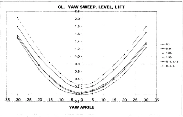
Figure 3 is a plot of the lift coefficient versus yaw angle for the same setups from figure 2. This set of tests was primarily focused on getting the car stable in a crosswind, since it was very unstable in 2003. By tilting the nose down, we reduced the lift and induced drag. The setup we chose to run with was zero-lift at zero-yaw. We established this success criterion from the GM Sunraycer case history wind tunnel tests for what the General Motors team established as a "safe" amount of lift in an ultra lightweight vehicle like ours. (Lissaman 22) They were comfortable with a lift area of 1.2 sq. m. With our chosen running configuration, our lift area was 1.16 sq. m.
CL, YAW SWEEP, LEVEL, LIFT
Of ... __.._ ..-..._... .. .. _---- -- . ... ..
,,*x~~~~
~
2.0
, \e -.- 0.1 "--0.34- 1.09-- 1.551.09-- 1.55--- 1.55---R-1, 1.13--. 5, 9-.i -3, ,,,,-,,,2,,,5,,,,,,,,,,,,-20,,,,,,,,,,, - -20,,0,,,,,,,,, ,-,,5,,-15 ,,15,,,,,,,,,, -10,,,,,, 51 20 25 30 3,,5 - . ... ... ... .... .... ... ...5. ... ... ... ... ..2 ...5 .... ... ... ... ... . ... ... ...30 ... ...5 YAW ANGLEFigure 3. Lift Coefficient versus yaw angle for various angles of attack.
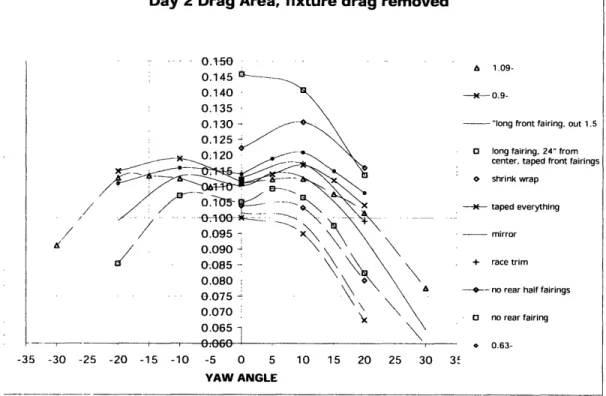
Figure 4 shows the drag area from the various setups from day 2. The main issues of importance from these tests were that sealing holes around the wheels and wheel fairings,
f i I ;; I : i i I
-and lengthening would reduce the head-on -and crosswind drag greatly. The positive drag slope I mentioned before disappears in the best-sealed, shrink-wrapped test setup.
Day 2 Drag Area, fixture drag removed
.. , 4
.A 1 n_
---
0.9---- "long front fairing. out 1.5
O long fairing, 24" from
center, taped front fairings
0 shrink wrap
X taped everything
mirror
+ race trim
0 -no rear half fairings 0 no rear fairing
-35 -30 -25 -20 -15 -10 -5 0 5 10 15 20 25 30 3'
YAW ANGLE
Figure 4. Drag area versus yaw angle for various test configurations.
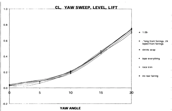
Figure 5 plots the lift coefficient versus yaw angle for the same test configurations as Figure 4. Note that details like fairing sealing, shrink-wrap, and mirrors don't affect the car's lift, only the main-body orientation can significantly change the lift coefficient.
. ./
---- ---
1.09-a ,"long front fairings, 24 taped front fairings
x Shrink wrap
v tape everything
+ race trim
· no rear fairing
YAW ANGLE
Figure 5. Lift Coefficient versus yaw angle at various test configurations.
Analysis
CdA vs. speed
80 90
Figure 6. CdA versus speed.
1 .0 0.8 0.6 0.4 0.2 0.0 -0.2 0.1200 0.1000 E 0.0800 O 0.0600 0.0400 0.0200 0.0000 30 40 50 60 Wind speed (mph) 70 n nn _ . U. 1IUU . .. ... ... ... ... ....
Figure 6 shows that there is little velocity dependence on the drag coefficient. It is customary to use a Reynolds number calculation for comparison, but by showing that these dimensions are best according to the rules, quoting a CdA is likely the best comparison amongst solar cars. Comparing our car's minimum drag at zero yaw, we matched that of Honda Dream '96, and was 30% better than the original GM Sunraycer. (Ozawa 349) (Lissaman 34)
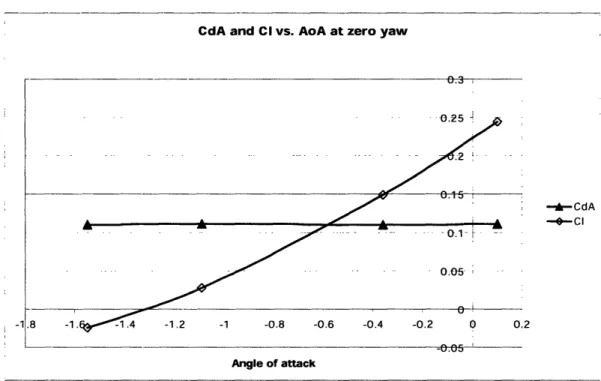
CdA and CI vs. AoA at zero yaw
-- CdA
0 Cl
Angle of attack
Figure 7. Lift and drag coefficients versus angle of attack.
Figure 7 shows lift and drag coefficients versus angle of attack, one of the primary criteria we chose to optimize. The drag coefficient changes very little with angle of attack at zero yaw, whereas the lift coefficient changes almost linearly. This allowed us to tune the vehicle's lift while leaving the zero-yaw drag untouched. There was some slight dependence of drag coefficient on angle of attack at a yaw, as shown in Figure 2.
I
The drag area plots are quite interesting, they are double humped, with a local minimum at zero yaw. The increase in drag from zero to 10 degrees yaw is likely due to internal flow around the front wheels. The Lexan plates around the wheel fairings don't quite seal very well, and in a crosswind, the side of the fairing can force air up inside the main body. After 10 degrees yaw, the slope is negative and the drag drops off. This is common with most modern solar cars, and is due to a crosswind drag reduction from the wheel fairings. In a crosswind, the foil-shaped fairings have an angle of attack, and therefore produce lift. This lift force can be resolved into the vehicle's coordinate system, which produces a large lateral component on the tire, and a forward component which helps to reduce the overall drag of the vehicle. University of Waterloo uses this feature greatly, with much larger wheel fairings that can actually change their camber based on the crosswind angle. (Thompson)
The parabolic shape of the lift coefficient vs. yaw plot is due to a flow-straightening effect of the wheels and wheel fairings. This was verified with the smoke wand tests at 20 degrees yaw. Across the top surface, the smoke followed the free stream direction, while across the bottom surface, the smoke followed the car's longitudinal axis. This is because the section of the car is a different lifting foil, and the straightened flow prevents a balancing force from being produced on the bottom side of the car. GM used strakes on the top of the car to attempt to correct this problem. (Lissaman 17-23) (Tamai 132-135)
Conclusion
All together, we reduced lift and drag by finding an optimal angle of attack, and then we found the best fairing setup possible, which further reduced drag. The main body drag is likely 3% lower than the configuration in WSC '03, and much safer due to less lift. The fairing study also suggests that the next car should implement a redesign the front fairings for another 5% possible improvement. Also, the transition data suggests we should recess the array to avoid a forward facing step that forces transition, and we should design for laminar flow over the array, because the panel surface is smooth enough except for the initial step.
References
Ozawa, Hiroyuki, Et. Al. "Development of aerodynamics for a solar race car." JSAE Review 19 (1998) 343-349.
Tamai, Goro. The Leading Edge: Aerodynamic Design of Ultra-streamlined Land Vehicles. Cambridge: Robert Bentley, 1999.
Lissaman, Peter, Et. Al. GM Sunravcer Case History. Lecture 2-2. Warrendale: Society of Automotive Engineers, 1990.
Drela, Mark. Personal Conversation. Thompson, Greg. Personal Conversation.
Appendix A - Test Matrix
Data filename DDDFQC 24Mar05 RunOl DDDFQC 24Mar05 RunO2 DDDFQC 24Mar05 RunO3 DDDFQC 24Mar05 RunO4 DDDFQC 24Mar05 Run05 DDDFQC 24Mar05 RunO6 DDDFQC 24Mar05 RunO7 DDDFQC 25MAR05 RUN01 DDDFQC 25MAR05 RUN02 DDDFQC 25MAR05 RUN03 DDDFQC 25MAR05 RUN04 DDDFQC 25MAR05 RUN05 DDDFQC 25MAR05 RUN06 DDDFQC 25MAR05 RUN07 DDDFQC 25MAR05 RUN08 DDDFQC 25MAR05 RUN09 DDDFQC 25MAR05 RUN10 DDDFQC 25MAR05 RUN11 DDDFQC 25MAR05 RUN12 DDDFQC 25MAR05 RUN13 DDDFQC 25MAR05 RUN14 DDDFQC 25MAR05 RUN15 DDDFQC 25MAR05 RUN16 Flow speed (mph) 60 60 60 60 60 60 60 60 60 60 30 60 60 60 60 60 60 60 60 60 60 60 60 Angle of attack (deg.) 0.128 0.128 -0.36 -1.09 -1.55 -1.13 -0.89 N/A -0.93 -0.63 -0.93 -0.93 -0.93 -0.93 -0.93 -0.93 -0.93 -0.93 -0.93 -0.93 -0.93 -0.93 -0.93 Ride Height (in.) 12.5 12.5 12.5 12.25 11.625 11.25 11.375 N/A 11.875 12.5 11.875 11.875 11.875 11.875 11.875 11.875 11.875 11.875 11.875 11.875 11.875 11.875 11.875 Yaw Angles (deg.) 0, +/-5, 10,15, 20, 30 0, +/-5,10,15, 20, 30 0, +/-5, 10, 15, 20, 30 0, +/-5, 10, 15, 20, 30 0, +/-5, 10, 15, 20, 30 0, +/-5, 10, 15, 20, 30 0, 5,10,15, 20, 30 0 0, 5, 10, 15, 20, -10, -20 0, 5, 10, 15, 20, -10, -20 0, 5, 10, 20 0 0, 5, 10, 15, 20, 30,-10, -20 0,5,10,15,20, 30, -10, -20 0, 5,10,15, 20, 30, -10, -20 0, 5,10,15, 20, 30, -10, -20 0, 5,10,15, 20, 30,-10, -20 0, 10, 20 0,10, 20 0, 10, 20 0,10, 20 0,10, 20 0,10, 20 other parametersboundary layer blower on
only rear wheel fixture installed in tunnel
comparable to day 1 run 4
test for Reynolds number dependence
tall rear fairing
long rear fairing
long rear half fairings on front wheels
long rear half fairings with tips out 1.5"
long rear half fairings with tips out
3"
long rear half fairings with tips 24" out from centerline
shrink-wrapped array back to canopy
same as above with holes around the tires taped
added a single mirror
race trim
removed rear half fairings added rear half fairings, removed rear fairing Shift Number 1 1 1 1 1 1 2 2 2 2 2 2 2 2 2 2 2 2 2 2 2 2 Run number 1 2 3 4 5 6 7 1 2 3 4 5 6 7 8 9 10 11 12 13 14 15 16 - _ - . . _ .. _ _I _