Assessing the relationship between macro-faunal burrowing activity and mudflat geomorphology from UAV-based Structure-from-Motion photogrammetry

HAL Id: hal-03021798

https://hal.archives-ouvertes.fr/hal-03021798

Submitted on 24 Nov 2020

HAL is a multi-disciplinary open access

archive for the deposit and dissemination of

sci-entific research documents, whether they are

pub-lished or not. The documents may come from

teaching and research institutions in France or

abroad, or from public or private research centers.

L’archive ouverte pluridisciplinaire HAL, est

destinée au dépôt et à la diffusion de documents

scientifiques de niveau recherche, publiés ou non,

émanant des établissements d’enseignement et de

recherche français ou étrangers, des laboratoires

publics ou privés.

burrowing activity and mudflat geomorphology from

UAV-based Structure-from-Motion photogrammetry

Guillaume Brunier, Emma Michaud, Jules Fleury, Edward Anthony, Sylvain

Morvan, Antoine Gardel

To cite this version:

Guillaume Brunier, Emma Michaud, Jules Fleury, Edward Anthony, Sylvain Morvan, et al.. Assessing

the relationship between macro-faunal burrowing activity and mudflat geomorphology from

UAV-based Structure-from-Motion photogrammetry. Remote Sensing of Environment, Elsevier, 2020, 241,

pp.111717. �10.1016/j.rse.2020.111717�. �hal-03021798�

Assessing the relationship between macro-faunal burrowing activity and

mudflat geomorphology from UAV-based Structure-from-Motion

photogrammetry

Article  in  Remote Sensing of Environment · May 2020 DOI: 10.1016/j.rse.2020.111717 CITATIONS 0 READS 156 6 authors, including:

Some of the authors of this publication are also working on these related projects:

Geomorphic evolution of the Makran coastView project

Gof-Boulders "Geomorphological control on offshore and onshore boulders transport along a wave dominated coast"View project Guillaume Brunier

24PUBLICATIONS   409CITATIONS   

SEE PROFILE

Emma Michaud

French National Centre for Scientific Research

32PUBLICATIONS   839CITATIONS   

SEE PROFILE

Jules Thomas Fleury

Aix-Marseille Université

70PUBLICATIONS   835CITATIONS   

SEE PROFILE

Edward Anthony

Centre Européen de Recherche et d’Enseignement des Géosciences de l’Environn…

327PUBLICATIONS   6,150CITATIONS   

SEE PROFILE

UNCORRECTED

PROOF

Remote Sensing of Environment

Assessing the relationship between macro-faunal burrowing activity and mudflat

geomorphology from UAV-based Structure-from-Motion photogrammetry

GuillaumeBrunier

_{, EmmaMichaud}

_{, JulesFleury}

_{, Edward J.Anthony}

_{, SylvainMorvan}

_,

AntoineGardel

a_{CNRS, Univ Brest, IRD, Ifremer, LEMAR, F-29280 Plouzane, France}

b_{UM 34 CEREGE, Aix Marseille University, CNRS, IRD, INRA, Collège de France, Aix-en-Provence, France}

c_{Laboratoire Ecologie, Evolution et Interactions des Systèmes Amazoniens (LEEISA), CNRS, Univ Guyane, Ifremer, 275 route de Montabo, 97334 Cayenne, French Guiana}

A R T I C L E I N F O

A B S T R A C T

Characterisation of the ecosystem functioning of mudflats requires insight on the morphology and facies of these coastal features, but also on biological processes that influence mudflat geomorphology, such as crab bioturba-tion and the formabioturba-tion of benthic biofilms, as well as their heterogeneity at cm or less scales. Insight into this fine scale of ecosystem functioning is also important as far as minimizing errors in upscaling are concerned. The re-alisation of high-resolution ground surveys of these mudflats without perturbing their surface is a real challenge. Here, we address this challenge using UAV-supported photogrammetry based on the Structure-from-Motion (SfM) workflow. We produced a Digital Surface Model (DSM) and an orthophotograph at 1 cm and 0.5 cm pixel reso-lutions, respectively, of a mudflat in French Guiana, and mapped and classed into different size ranges intricate morphological features, including crab burrow apertures, tidal drainage creeks and depressions. We also deter-mined subtle facies and elevation changes and slopes, and the footprint of different degrees of benthic biofilm development. The results generated at this scale of photogrammetric analysis also enabled us to relate macrofau-nal crab burrowing activity to various parameters, including mudflat elevation, spatial distribution and sizes of creeks and depressions, benthic biofilm distribution, and flooding duration. SfM photogrammetry offers interest-ing new perspectives in fine-scale characterisation of the geomorphology, benthic activity and degree of biofilm development of dynamic muddy intertidal environments that are generally difficult of access. The main short-comings highlighted in this study are a drift of accuracy of the DSM outside areas of ground control points and the deployment of which perturb the mudflat morphology and biology, the water-logged or very wet surfaces which generate reconstruction artefacts through the sun glint effect, and the time-consuming task of manual in-terpretation of extraction of features such as crab burrow apertures. On-going developments in UAV positioning integrating RTK/PPK GPS solutions for image-georeferencing and precise orientation with high-quality inertial measurement units will limit the difficulties inherent to ground control points, while conduction of surveys dur-ing homogeneous cloudy conditions could reduce the sun-glint effect. Manual extraction of image features could be automated in the future through the use of deep-learning algorithms.

1. Introduction

Biogeomorphology is the study of interactions between geomorphic processes and biota (Naylor et al., 2002). In coastal systems, whereas some organisms enhance sediment erosion (e.g., molluscs), others con-tribute to sediment accumulation and coastal protection (e.g., benthic microalgae, mangroves, salt marshes, coral and worm reefs). For in-stance, benthic microalgae (e.g., diatoms) occur in regularly-spaced patterns consisting of elevated hummocks alternating with

water-logged hollows, enhancing sediment cohesion and stabilisation (Van De Koppel et al., 2001; Weerman et al., 2010). However, destabili-sation of cohesive sediments may be promoted by macrofaunal biotur-bation activities (e.g., sediment mixing, burrowing and irrigation pat-terns) including microphytobenthos consumption, which directly affects sediment porosity and permeability (Orvain et al., 2004; Rhoads and Young, 1970; Widdows et al., 1998). In some cases, crab bio-turbation enhances saltpan formation and tidal creek extension, thus driving the local geomorphic patterns (Escapa et al., 2007). Where grazing on microphytobenthos by benthic macro-invertebrates is

⁎_{Corresponding author at: Laboratoire des Sciences de l'Environnement Marin (LEMAR), UMR 6539 (UBO/CNRS/IRD/Ifremer), Institut Universitaire Européen de la Mer, rue Dumont}

d'Urville, 29280 Plouzané, France.

E-mail address: guillaume_brunier@hotmail.fr (G. Brunier) https://doi.org/10.1016/j.rse.2020.111717

Received 1 November 2019; Received in revised form 4 Febraury 2020; Accepted 8 Febraury 2020 Available online xxx

UNCORRECTED

PROOF

variability and that of the associated sediment structural properties are generated at scales of up to several metres that are large enough to affect landscapes (Pratt et al., 2015; Sommer, 2000; Weerman et al., 2011). Ideally, however, a biogeomorphic system should be seen as a two-way interaction system wherein geomorphic processes and land-forms affect the distribution of biota, and conversely, biota modify geo-morphic processes and landforms (Stallins, 2006).

In this two-way interaction system, geomorphic patterns are not lin-ear due to the high variability of the distribution of benthic organisms, which is attributed to the ‘patchiness’ effect (Grünbaum, 2012). Such spatial heterogeneity occurs naturally in ecosystems and is maintained by spatio-temporal variations in a range of physical conditions in areas subjected to the impacts of benthic activity. Crab communities and their bioturbation intensity, for instance, vary as a function of tidal range, vegetation structure, microhabitat, and seasonality (Aschenbroich et al., 2016; Cannicci et al., 2018; Escapa et al., 2007; Li et al., 2018). The spatial scales of patchiness in the variables being measured are often not known before sampling.

Such patchiness and heterogeneity of the environment can, when underestimated, lead to significant errors in extrapolations aimed at upscaling. Because heterogeneity of the environment usually increases with scale, extrapolations that do not incorporate this heterogeneity are subject to inaccuracy. Increasing the number of replicates in a large site

does not necessarily make up for within-location variability, which can be more important than inter-site variability (Morrisey et al., 1992). The characterisation of the functioning of an ecosystem and of biogeo-morphic interactions, therefore, necessarily requires a good knowledge of small and medium-scale processes in order to minimise errors in up-scaling. Such processes are, however, difficult to assess in highly dy-namic sedimentary environments subject to recurrent disturbances. This is notably the case on wave-exposed coasts subject to large supplies of mud, as in certain tropical environments such as deltaic mangroves and mudflats (Brunier et al., 2019).

The French Guiana coast (Fig. 1) in South America is part of the longest muddy coast in the world (1500 km) and is strongly influ-enced by mud banks migrating NW from the mouths of the Amazon to those of the Orinoco. Rapid colonisation of these mud banks, com-monly over several tens of km2_{a year, by mangroves, and bank} consol-idation (termed the bank phase), are generally followed by rapid bank erosion (the inter-bank phase) a few years later (Anthony et al., 2010). The ensuing spatially and temporally varying shoreline changes reflect complex interactions between hydrodynamic, morphodynamic, rheolog-ical and biologrheolog-ical processes. The welding onshore of a mud bank in-volves the formation of mud bars and mudflats that are colonised by mangroves, generating an environment rapidly impacted by benthic ac-tivity. These muddy deposits and their colonizing mangroves dissipate wave energy, enabling further progressive muddy coastal accretion. Ap

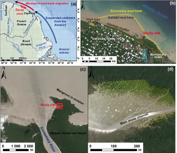
Fig. 1. Regional context of study site: (a) western sector of the Amazon mud belt from the mouths of the Amazon (Brazil) to Suriname; (b) mud bank at the Sinnamary river mouth seen

on a Landsat 8 OLI image dated September 2015, one month prior to the field survey; (c, d) location of the study site on the east side of the river mouth in the inner part of the mud bank fronted by young and mature mangrove forests. Images are from Pleiade MS (© CNES, 2015) and Astrium Services/PLEIADES (17/09/2015) - not for commercial use); the brighter sharp-focus area superimposed on the background Pleiade image in (d) is a large-scale orthophotograph produced from a UAV survey in the course of the field experiment. It shows the dense network of mudflat creeks and depressions, and progressive mangrove colonisation.

UNCORRECTED

PROOF

inter-tidal substrate is difficult to access in the field and characterised by cen-timetre-scale spatial habitat and biogeomorphic variability (Anthony et al., 2008, 2014; Proisy et al., 2009; Aschenbroich et al., 2016, 2017). These two aspects limit the possibilities of characterisation of benthic variables, even when high-resolution and accurate surface-map-ping techniques such as RTK-DGPS, terrestrial LiDAR (TLS), or a total station are used.

Remote-sensing methods such as multispectral or hyperspectral map-ping from satellite or aircraft images, constitute, on the contrary, an excellent tool for characterizing biogeomorphic variability and predic-tion of microphytobenthos and macrobenthos distribupredic-tions (Adolph et al., 2017; Kazemipour et al., 2012; Méléder et al., 2003; van der Wal et al., 2008, 2010). These methods, the advantages of which lie in the remotely-sensed data acquisition, encompass a large range of techniques that are ideally applicable at various spatial and tempo-ral scales, and costs. In addition to classical optical and radar satellite images, spatial and temporal ecosystem characterisation is now being routinely carried out using airborne LiDAR (Okyay et al., 2019) and photogrammetry (Anderson et al., 2019), the latter from a variety of platforms such as unmanned aerial vehicles (UAV), microlight aircraft, kites and poles. Breakthroughs in the handling, managing and visual-isation of large point clouds generated by these modern remote-sens-ing techniques have opened up new perspectives in characterizremote-sens-ing the biogeomorphology of ecosystems, notably enabling the generation of maps of various types (vegetation cover, bed-surface characteristics, topography, etc.), digital elevation models (DEMs), or digital surface models (DSMs) that include, in addition to terrain elevation, miscella-neous surface information such as vegetation, buildings and infrastruc-ture. However, each of these techniques has operational and quality constraints in terms of cost and reproducibility, coverage, point den-sity and accuracy (Passalacqua et al., 2015). Barring the question of cost, the only two techniques applicable to muddy coastal environments and their commonly variable fine-scale topographic and benthic vari-ability are LiDAR and airborne photogrammetry. Airborne LiDAR has set the standard for surveying mudflat landscapes at decimetre- to me-tre-scale resolutions. The method allows for rigorous mapping of mud-flat morphometry, including, for instance, channel geometry and bed erosion through laser penetration into the water column (Brzank et al., 2008a, 2008b; Okyay et al., 2019). Airborne LiDAR is, however, costly, can be of limited applicability in highly turbid waters, and re-peated surveys are not adapted for small areas of muddy environments and their characterisation at a very fine scale that aims at bringing out micro-topographic and benthic variability (Proisy et al., 2009). Zhao et al. (2019) used a terrestrial laser scanner embarked on a hover-craft and attained the resolution needed for monitoring micro-geomor-phology and bioturbation processes on a mudflat, but this survey proce-dure is highly time-consuming, extremely limited in its spatial coverage, and yields less accurate results. Photogrammetry is an old remote sens-ing technique notably used in the past to produce topographic informa-tion and orthophotographs. Hitherto an elaborate and tedious method, it has evolved with the development of computer-assisted techniques, notably the so-called Structure-from-Motion (SfM) workflow (Westoby et al., 2012) combined with the use of lightweight and flexible carriers such as UAVs, microlight aircraft, helicopters or kites (Bryson et al., 2013; Tonkin et al., 2014; Brunier et al., 2016a). SfM photogram-metry uses standard cameras for photography and bundle-block adjust-ment algorithms that align pictures together and produce a three-di-mension (3D) point cloud in a relative or absolute 3D reference (James and Robson, 2012, 2014), enabling the production of high-resolu-tion models and derived products such as DSMs and orthophotographs. These new developments have led to the emergence of SfM photogram-metry as a low-cost, reproducible and high-resolution alternative to lasergrammetry techniques or traditional topographic survey tech

niques (Anderson et al., 2019). Up to now, photogrammetry has, with very exceptions, hardly been used in muddy water-saturated environ-ments with unstable substrates and that are generally difficult of access. Recent applications have concerned temperate (Jaud et al., 2016) and tropical (Brunier et al., 2016b) mudflats, and temperate saltmarshes (Doughty and Cavanaugh, 2019; Kalacska et al., 2017).

The aim of this study is to characterise, at a very fine resolution using photogrammetric techniques, the biogeomorphic processes on a tropi-cal intertidal mudflat in French Guiana. SfM photogrammetry, based on UAV surveys, was used to highlight the biogeomorphic relationships be-tween the apparently uniform and monotonous topography of a rapidly changing mudflat and its biological imprints, notably benthic biofilms and bioturbation activities associated with crab burrows.

2. Materials and methods 2.1. Study area

The field experiment was carried out between 29 September and 3 October 2015, in the course of spring tides at low tides, over an inter-tidal area of 1 ha on the Sinnamary mud bank at the mouth of the Sin-namary estuary (Fig. 1) where pioneer mangrove colonisation started early in 2015. The study site shows three levels of mud deposits: (1) fresh water-saturated mud during low tide and exhibiting a very smooth surface, (2) consolidated mud drained by variably sized creeks at low tide and characterised by numerous depressions, and (3) bare consoli-dated mud that may be colonised by mangroves in places. Colonisation typically results in the establishment of a fringe of young mangroves.

The Sinnamary estuary is a macro-tidal, semidiurnal type with spring and neap ranges of 2.1 ± 0.3 m and 1.3 ± 0.3 m, respectively, and spring and neap high-tide water levels of 3.2 m and 2.8 m, respectively, above local hydrographical vertical datum.

2.2. UAV-based field survey and SfM photogrammetry workflow 2.2.1. Field surveys

In order to observe in detail the biogeomorphology of the pioneer mangrove area and its spatial variability, the operational protocol based on aerial photography was complemented by field measurements of the spatial locations and elevations of ground control points (GCPs) and ground truth points (GTPs) (Table 1 & Fig. 2). A UAV DJI F550 hexacopter was used with a Ricoh GR camera mounted on a gimbal. The flight duration was 12 min and the area coverage per flight was

Table 1

Summary of experimental settings.

UAV model DJI F550

Camera

Model RICOH GR

Resolution 20MP

Focal 18.3 mm (fixed)

Flight

Height above ground 18 m

GSD 4.6 mm

Flight duration 12 min

Coverage 3 ha Number of pictures 265 GCP settings Number 26 Elevation accuracy 0.03 m Method RTK-DGPS

UNCORRECTED

PROOF

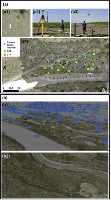
Fig. 2. Drone-based SfM photogrammetry work-flow stages: (a) field operations conducted

prior to the aerial photographic survey: (a1) dropping off of GCPs and GTPs and (a2) their georeferencing at the centimetre-scale using RTK-DGPS; (a3) aerial survey settings of the UAV system used: DJI F550 model with embarked Ricoh GR professional compact camera; (a4) GCPs, GTPs and camera centre location layout for this survey. (b) SfM photogram-metry using Agisoft Photoscan program involving a two-step aerial triangulation: (b1) 3D view of the position and orientation of pictures in the scene with the sparse point cloud; (b2) dense-point cloud generation using dense stereo multi-view reconstruction. 1.2 ha. The Ricoh GR is a high-end compact lightweight (243 g) camera well suited for drone deployments. It has an APS-C sensor and a sharp quality inbuilt lens with a fixed focal length of 18.3 mm and various customisable functions such as a shooting interval meter. The camera settings for the flight were a focus set to infinite, a high shutter speed of 1/2500 s to avoid image motion-blur due to UAV speed, a low ISO value for image quality, and an aperture of f/4.5 to f/8 to limit diffrac-tion and increase image contrast in view of the local brightness condi-tions. The camera shooting interval was triggered at 1 s, and pictures were recorded in RAW format and then converted to JPEG format with-out compression for further processing. For reconstructing the 3D mud-flat geometry at very high resolution and obtaining a sub-centimetre

resolution for orthophotographs, a flight plan was defined at a very close range of 18 m above the ground. This flight height was chosen as it al-lowed for a very fine pixel Ground Size Dimension (GSD) of 4.6 mm with respect to camera focal length and sensor dimension. Water sur-faces in small depressions and creeks create local topographic artefacts due to sun glint. To operate stereo-image matching, standard frontlap and sidelap ratios of respectively 90 and 60% were considered. 265 pho-tographs were taken during each flight. The survey flight plan was de-signed using DJI Ground Station Professional program. Although the UAV path covers the mudflat homogeneously, the camera trigger at 1 s interval saturates the camera recording process during some part of the flight, resulting in several, but spatially limited, gaps in pho-tography. Prior to the flight, 26 GCP and GTP targets each made of 0.5 × 0.5 m plywood board with an easily discernible black-and-white checker-board pattern were dropped off on the mudflat. Their positions were measured using a Trimble © R8 RTK-DGPS with the base antenna fixed on a stable horizontal board. The GCPs were used, first, to enable absolute referencing of the produced 3D model, second, to estimate ex-trinsic and inex-trinsic parameters of the camera in the photogrammetric workflow, and, third, to assess the horizontal and vertical accuracies of subsequently generated DSMs. The GTPs were also used in a comple-mentary assessment of these accuracies. Deployment of the GCPs and GTPs was tricky over the unstable muddy terrain. As a result, these were essentially deployed over only a part of the mudflat area between two main creeks (Fig. 2).

The topographic survey was operated in the projected Coordinate Reference System (CRS) Universal Transverse Mercator (UTM) zone 22 North Hemisphere, related to the Geodetic Network of French Guiana 1995 datum (RGFG 1995 in French; EPSG: 2172). The Earth Gravita-tional Model 2008 (EGM 2008) was used as elevation datum.

2.2.2. SfM photogrammetry and orthophotograph/DSM production A standard SfM photogrammetry pipeline (Lucieer et al., 2014; Turner et al., 2014), using Agisoft © Photoscan Professional program version 1.2.6 (Table 2 & Fig. 2), was used to build the 3D model and export the end-products. After selection of the non-redundant and good-quality pictures, we initiated the aerial triangulation in a first step named “image alignment” which consisted in: (1) extraction of the key points on each image using a Scale Invariant Feature Transform-like (SIFT) algorithm (Lowe, 2004; Turner et al., 2014); (2) finding all matching tie points in image pairs; (3) processing the self-calibration starting from a basic camera model using the Exchangeable image file format (Exif) information and refining it using the tie points; (4) cal-culating the relative orientation of cameras using bundle-blocks adjust-ment. This step created a first 3-D sparse tie-point cloud that was then filtered from outliers using a thresholding re-projection error at 1 pixel, and then from manual deletion of erroneous tie points from their posi

Table 2

Setting and quality assessment of SfM photogrammetric products. SfM photogrammetry: processing results

Number of cloud points 123 × 10^6 points

Dense cloud density 11,600 points/m2

Mesh face number 24 × 10^6

DSM resolution 1 cm/pixel

Orthophotograph resolution 0.5 cm/pixel

Number of GCPs used 14

Number of GTPs used 12

Geometric accuracy for Orthophotograph and DSM

Tie-point reprojection error 0.6 pixel

GCP-reprojection error 0.4 pixel

RMSE of horizontal accuracy 0.022 m

UNCORRECTED

PROOF

the GCPs in each image allowed an “optimisation” procedure which con-sisted in a refinement of the camera calibration model and of the spa-tial position and orientation of the cameras, based on photogrammetric measurements of the projections of the GCPs in the images. The centres of 14 of the 26 targets were then picked up on the photographs and used as GCPs. By virtue of these GCPs, the 3-D scene geometry was integrated into the CRS of the study area before being optimised. The average re-projection error of tie points after this step was 0.6 pixels. From the estimated GCP locations on the model, compared to the measured ones, the programme estimated the mean residual of the 3D model at 0.02 m (Table 2). The final 3-D geometry scene, named “dense point cloud”, was created using the dense multiview stereo reconstruction algorithm (Furukawa and Ponce, 2010) with a high quality setting in the pro-gramme, meaning half-resolution downscaling of each image. The point cloud density was close to the range generally obtained with terrestrial LiDAR. A polygonal 3-D model, named mesh, was built from 3-D trian-gulation applied to the dense point cloud in order to produce oblique textured scene views. The dense 3D point cloud was filtered for outliers, and then interpolated to create a gridded DSM that reproduced all ob-jects present on the photographs (such as vegetation, human artefacts), along with an orthophotomosaic, at resolutions of 1 cm and 0.5 cm per pixel, respectively. Twelve GTPs were used to assess the quality of the 3D model geometry. More detailed information on SfM-photogrammet-ric processing can be found in Brunier et al. (2016a), James and Robson (2012, 2014), Jaud et al. (2016), Lucieer et al. (2014), and Turner et al. (2014).

2.3. Biogeomorphic analysis 2.3.1. Mudflat geomorphic units

Geomorphic units were identified and classified from orthophoto-graph, DSM, and derived products (Fig. 3). Steep and planar areas were extracted using surface roughness calculation based on the stan-dard deviation of elevation over 15 × 15 neighbouring cells in each DSM. This index represented the variability of DSM cell elevation rela-tive to neighbouring cells: when the standard deviation increased, the elevation changes also increased. Cells with a standard deviation of el-evation above 0.02 m were used to delimit steep sloping surfaces (Fig.

3c). Morphological limits based on these steep surfaces were digitised in combination with orthophotographs and contours at an interval of 0.02 m in the case of smooth surfaces, thus enabling the identification of various geomorphic units (Fig. 3d). This workflow was conducted with the Geographic Information System program ESRI ArcGIS desktop v 10.2.

2.3.2. Tidal flooding duration and number of flooding occurrences The flooding duration was calculated in hours during mean spring and neap tides as a function of substrate elevation. The tide water level was calculated with an interval of 15 min. From conversion of tide wa-ter level to local vertical datum (here NGG 77), DSM pixels below the water level were selected by thresholding, using the GIS program. This operation resulted in a binary image where each pixel is considered as flooded or not for each input tide water level. The binary images of the flooded surface were then summed up pixel per pixel to calculate the number of flooding occurrences. These occurrences were multiplied by tide water level interval, here 15 min, to obtain the flooding duration. The Sinnamary estuary is not equipped with a tide gauge. To obtain a tidal record, the intertidal water level records obtained in situ from a pressure gauge were compared to those of the tide model of the Salva-tion Islands, about 50 km offshore SE of the estuary. Comparing the two curves we observed that the high tide peak of Salvation Islands was 17 to 20 min earlier than that from the local measurements. Using the ele-vation of the pressure gauge at 0.45 m NGG77, the recorded water levels were corrected in NGG vertical datum, and an offset of −2.19 ± 0.07 m was calculated to correct the simulated water levels at the Salvation Is-lands relative to our position. This enabled the estimation of the mean spring and neap tide level observations in local vertical datum NGG77 with respective values of 1.1 m and −1.14 m for spring tide high and low tide levels, and 0.5 m and −0.64 m for high and low neap tide lev-els. These tide ranges and a mean cycle duration of 12 h15 were used as inputs in the following formula (Eq. (1)) in order to generate water level tables, with a 15-minute time step:

where h is the calculated water level (m), A the tide range (m), T the cycle period (hours), φ the tidal phase and H the initial height (m).

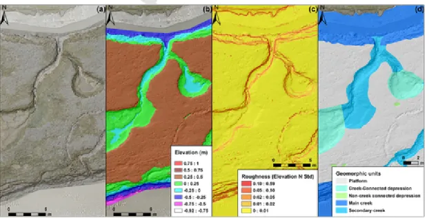
Fig. 3. Methodology for the contouring of geomorphic units from a very high-resolution DSM: (a) orthophotograph with hillshade of DSM background; (b) DSM showing sediment

ele-vation over a segment of the study area highlighting the presence of creeks, platform and depressions; (c) raster of surface roughness determined from standard deviation of eleele-vation calculated for each DSM cell with reference to its 15 × 15 neighbours, highlighting clearly surfaces with steep slopes; (d) geomorphic units photo-interpreted from the elevation standard deviations, DSM and orthophotograph.

UNCORRECTED

PROOF

duration over the generated DSM topography during mean spring and neap tides.

2.3.3. Surface sediment colour from orthophotographs

A supervised classification of the visible colour of surficial mudflat areas was realised from the orthophotgraph in order to assign to each pixel its appropriate and homogeneous colour classes. The Orfeo Tool-box package and its graphical interface MonteVerdi, developed by the French National Centre for Space Studies (CNES), were used for this operation. Four classes of surface facies, each of which corresponds to an intensity of biofilm development on the mudflat, were identified on the orthophotographs (Fig. 4): facies 1 (F1) - dark green surfaces at-tributed to well-developed benthic biofilm; facies 2 (F2) - light green surfaces corresponding to moderately developed biofilm; facies 3 (F3) -ochre surfaces corresponding to soft mud with poorly developed biofilm; and facies 4 (F4) - grey surfaces corresponding to bare dry and wet mud without biofilm or with small patchy biofilm. Before processing the classification, water surfaces were masked since they were highly turbid and thus induced confusion with bare mud surfaces. Continu-ous mangrove stands, which can be confused with F1 and F2 facies because of their canopy colour, were also masked by manual digitisa-tion and removed from the analysis. However, the locadigitisa-tions of individ-ual mangrove trees, and small sparse patches of mangroves, as distinct from continuous stands, were included in the figures in order to give a visual idea of the stage of mangrove colonisation of the mudflat. The colour-reconnaissance was made from a single Red-Green-Blue (RGB)

image, and using the machine-learning “random forest” algorithm which is known to be rapid and efficient with high-resolution datasets (Inglada et al., 2015), and easy to tune compared to other more dif-ficult methods such as Support Vector Machine (SVM). The complete workflow is as follows: (1) computation of sample statistics; (2) selec-tion of samples in order to have a homogeneous sample distribuselec-tion per class; (3) extraction of sample measurements; (4) computation of im-age statistics; (5) training of a machine-learning classifier using selected samples (random forest algorithm) configured with a maximum of 100 trees, 10 features on each node, and a minimum of 10 samples per node; (6) running of the image classification; (7) cleaning-up of the classifica-tion image; (8) validaclassifica-tion of the classificaclassifica-tion model. The spatial distri-bution of the four colour classes was analysed in association with the geomorphic units, elevation, slope range, tidal flooding duration, and proximity to creeks and depressions. The information derived was built into an orthometric grid of points covering the area of interest. The grid points were spaced at an interval of 0.025 m, which is larger than that of the orthophotograph resolution (0.005 m), in order to reduce calcu-lation time, and then for each node the surface class and topographic information were extracted.

2.3.4. Spatial analysis of crab burrow aperture network

An important biogenic imprint on the surface of the mudflat and pi-oneer mangroves reflecting significant bioturbation is that of the nu-merous burrow apertures of fiddler crabs of the Uca gender (Aschen-broich et al., 2016). Burrowing fiddler crabs create sub-surface gal-leries below surface apertures of various sizes. Using the 0.5 cm resolu

Fig. 4. Classification of surface facies based on their dominant colour on the orthophotograph: (a) extraction of the main facies chosen visually (dark green, light green, ochre, grey), and

used to process RGB colour classification using QGIS's Orfeo Tool Box; (b) an example of results from the colour supervised classification. (For interpretation of the references to colour in this figure legend, the reader is referred to the web version of this article.)

UNCORRECTED

PROOF

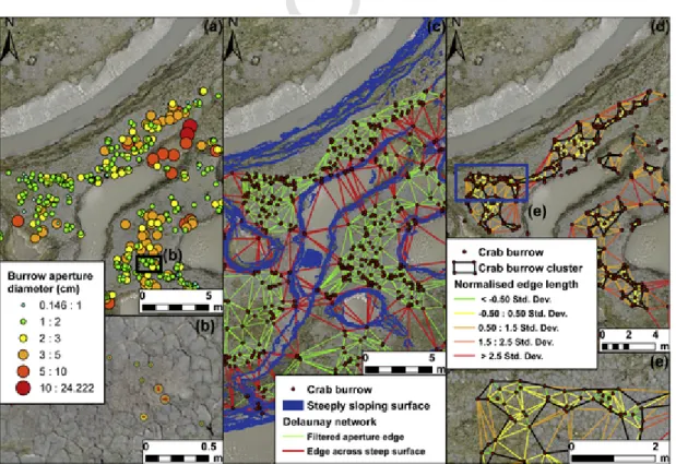
de-termined using GIS. Aperture locations and diameters were first digi-tised by photo-interpretation, and indexed into 3 size classes according to their diameter: small (S), with a diameter < 2 cm, medium (M), from 2 to 5 cm, and large (L) > 5 cm (Fig. 5). For each aperture, we ex-tracted, automatically, elevation, slope, and geomorphic unit (see Fig. 3d for units). To assess the spatial distribution of aperture size classes, the distance between neighbouring apertures was calculated using De-launay triangulation spatial functions that build irregular triangular net-works (TIN) from discrete points in a plane where each edge connects an aperture location with its closest neighbours. Edges between apertures were filtered in order to extract significant and reliable connections. The TIN was, in the first place, constrained to the area of interest using a mask. Within this area of interest, abnormal edges connecting two aper-tures distant > 10 m or crossing steep surface feaaper-tures (such as creek banks) and water-logged creeks were removed. Based on the assumption that the active ‘space’ of an individual fiddler crab rarely exceeds 1 m2 and on the fact that such crabs do not cross the creeks because of sub-strate instability and the steep bank creeks (Zeil and Hemmi, 2006), pixels representing steep slopes were used to create polygon layers (Fig. 3c). Edges intersecting these polygons were removed. Finally, the se-lected edges were grouped into six classes: a small aperture connecting with another small aperture, a small with a medium-sized one, a small with a large, a medium-sized with a medium-sized, a medium-sized with a large, and a large with a large. Edge distance was calculated to analyse the clustering and the dispersal of the aperture size classes using classi-cal index parameters such as variance and standard deviation. For this, each aperture was assumed to be an individual one within the spatial cluster according to the variability of edge distances: with a standard de-viation of edge distance < 0.5, which corresponds to 0.87 m, the edges were considered clustered. This enabled selection of edges and apertures of a same cluster.

3. Results 3.1. DSM quality

The very high resolution of the point acquisition comes out in a sin-gle point cloud with 11,600 points per m2_{. The mesh model was} deci-mated to 24 million faces, allowing for the construction of the DSM at 1-cm cell resolution. The general accuracy of the 3D model reached a high precision with re-projection errors, expressed in photo pixels, of 0.6 and 0.4 pixel for tie points and GCPs locations respectively. The eleva-tion comparison between GCPs and GTPs and the DSM yielded a Root Mean Square Error (RMSE) of 3 cm with 2 cm for planar error and 2 cm for elevation, a magnitude equivalent to the uncertainty of our measure-ments using RTK-GPS (Table 2). Due to the lack of evenly distributed GCPs, the borders of the DSM were affected by a deformation termed the “bowl effect” in the literature (Brunier et al., 2016a; Ouédraogo et al., 2014). To obviate this problem as well as the slight discrepan-cies in the UAV flight paths, the DSM was cropped and the analysis was limited to the area of the mudflat covered by the GCPs.

3.2. Mudflat geomorphology and flooding duration

Five geomophic units were identified and their percentage cover-age of the mapped area calculated: (1) a mud platform, characterised by a plane surface (54.8% of the mapped area), (2) main creeks with 0.7 m-high banks and bottom widths > 3 m (22.5%), (3) secondary creeks with bottom widths < 3 m (8%), (4) depressions connected to the secondary creek network (13.6%), and (5) unconnected or incipi-ent depressions (1.1%) (Fig. 6). The largest and deepest depressions are connected to the secondary creek network. Hence the use of the cri-terion of connectivity with the hydrographic network for distinguish-ing two types of depressions. The platform is the dominant mudflat unit, and forms a sub-horizontal surface lying at an average elevation of

Fig. 5. Analysis of the spatial distribution of the burrow apertures: (a) example of burrow aperture distribution over the mudflat; (b) burrows classified according to aperture size; (c)

Delaunay triangulation network of apertures enabling calculation of proximity statistics between aperture classes and identification of community clusters as a function of inter-cluster distance and local morphology; (d) and (e) filtered edge network classified on the basis of the standard deviation of edge length values normalised relative to the longest edge.

UNCORRECTED

PROOF

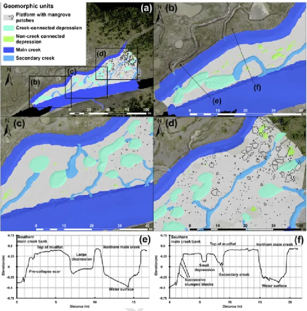
Fig. 6. Mudflat geomorphology: (a) area of interest with the five geomorphic classes: platform in light grey with individual mangrove trees or patches of mangroves, connected pools in

cyan, unconnected pools in light green, secondary creeks in light blue and main creeks in dark blue; (b–d) parts of mudflat enclosed by main creek channels from the narrowest in the SW to the largest in the NE; (e–f) Topographic profiles (see locations in panel b), illustrating the diversity of morphology and processes occurring over this mudflat (the term water surface corresponds to an area where the channel bottom has not been mapped). (For interpretation of the references to colour in this figure legend, the reader is referred to the web version of this article.)

0.4 m (Fig. 6) with a very gentle variation from 0.35 m at the SW limit of the study area to 0.5 m at the NE limit close to the young mangrove forest. This represented a mild slope ratio of 0.15%. The hydrographic network was composed of two main creeks fringing the platform in the N and S, the latter representing the main flood tidal entry pathway. El-evations ranged from 0.4 m in the main N channel to 0.3 m in the main S one, yielding a slope ratio of 0.5%. The platform exhibited a dense network of desiccation mud cracks, and was dissected by an additional 15 secondary creeks ranging in depth from 10 cm to 50 cm. 76 depres-sions were identified, 66 of which were located in the narrow SW and central parts of the platform between the two main creeks. The 14 de-tected larger and deeper depressions (3 to 4 m wide and 0.2 to 0.4 m deep) represented 18.5% of the total, and were connected directly to the creek network or inter-connected by small creeks. These depressions commonly exhibited abrupt banks and sometimes gently sloping ramps where they were connected to the banks of secondary creeks. 62 un-connected depressions (0.4 to 1 m wide, and 5 to 15 cm deep), rep-resenting 81.5% of the observations, were mainly located in the SW and centrals part of the platform. Steep banks and collapse features lin

ing the creeks and larger depressions, such as longitudinal scars and slumped blocks, highlighted active destabilisation of the mudflat.

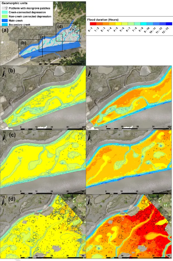
The flooding duration over the mudflat (Fig. 7) varied significantly, as expected, depending on spring or neap tides and elevation. Flooding duration of the platform during high spring tides ranged from 4 to 5 h, except in the most elevated areas colonised by mangroves (this higher elevation has been reported by Anthony et al. (2008) to reflect more active mangrove-induced sedimentation), which were flooded for only 3 to 4 h. Creeks and depressions were flooded over 5 to 8 h depending on depth. Platform flooding was more variable during neap tides: durations ranged from <1 to 3 h in the eastern sector depending on elevation, 3 to 5 h in the central sector rich in creeks and depressions, and 2 to 4 h over the rest of the platform. Creeks and depressions were flooded 4 to 8 h depending on depth and connectivity.

As observed on the orthophotograph, creeks and depression toms were not completely drained and dry during low tide. Creek bot-toms were in fact characterised by residual flow due to drainage of the mudflat. Non-creek-connected depressions remained water-logged dur-ing low tide, except for a number of small depressions that were drained through evaporation. The creek-connected depressions were usually

UNCORRECTED

PROOF

Fig. 7. Flood duration over the mudflat during spring and neap tides: (a) overview of mudflat geomorphology; parts of the mudflat (b–d) where flooding durations in hours for mean

spring (left panels) and neap tides (right panels) were mapped.

drained by outflow. As a result, large creek-connected depressions with bottom elevations close to or below creek bottom elevation were well drained. Large creek-connected depressions with bottom elevations lower than those of creek bottoms were only partially drained by out-flow and thus remained partially water-logged during low tide.

UNCORRECTED

PROOF

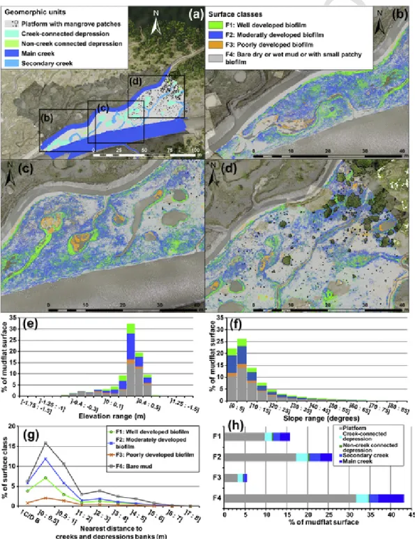
The map of surface colour classes (Fig. 8) depicts the distribution of biofilm facies and mangroves. At the scale of the study area, the facies units represent 15.8% for F1, 25.9% for F2, 5.5% for F3, 43.2% for F4 and 7.5% for water-logged areas (depressions and creeks) (Fig. 8).

F1 was abundant at an elevation of −0.2 to 0.5 m with no slope range preference (Fig. 8), and a flooding duration of 4 to 7 h during spring tides, and 2 to 7 h during neap tides (Fig. 7). This facies was lo-cated mainly within a distance of 1 m from creek and depression banks

or non-creek-connected depressions (Fig. 8). These characteristics sug-gest that this colour class was strongly related to humidity, in conti-nuity with creek and depression banks and bottoms. A diffuse distri-bution also appeared over the platform in the proximity of small and unconnected depressions in the SW sector or where local elevation de-creases occurred, such as in incipient creeks. F2 dominated over the mudflat, and was abundant between −0.2 to 0.5 m without a preferen-tial slope range, and with a same tidal range duration range as F1. F2 was especially prominent in the SW and central sectors of the mudflat where bare mud surfaces were rare. As in the case of F1, F2 was located within 1 m from creeks and depressions. F3 was the least represented

Fig. 8. Surface coverage by facies units: (a) overview of mudflat geomorphology; (b-d) parts of the area of interest with mapped surface facies classes. F1: highly developed biofilm, F2:

moderately developed biofilm, F3: poorly developed biofilm, F4: bare dry or wet mud, or with small patchy biofilm. The graphs show the distribution of facies classes in % of the area of interest: (e) elevation; (f) slope; (g) nearest distance to creek and depression banks; (h) geomorphic units.

UNCORRECTED

PROOF

established on the relatively mildly sloping (0 to 15°) bottoms of depres-sions and creeks. F3 was also located mainly within 1 m of creeks and depressions. Tidal flooding duration above F3 surfaces ranged from 4 to 8 h during spring tides and 2 to 10 h during neap tides. F4 was the most represented colour facies, and exhibited variable elevation, slope, and flooding duration ranges over the mudflat. The mangrove stand in the study site was mainly composed of young pioneer specimens with sparse saplings and small-diameter canopy size (<1 m) trees in the cen-tral and eastern parts of the platform, and trees with a >1 m-wide canopy size in the eastern border of the site. The pioneer saplings were

associated with a mudflat elevation ranging from +0.3 to +0.75 m. Large patches of F2 occurred around these saplings.

3.4. Spatial distribution of burrow apertures

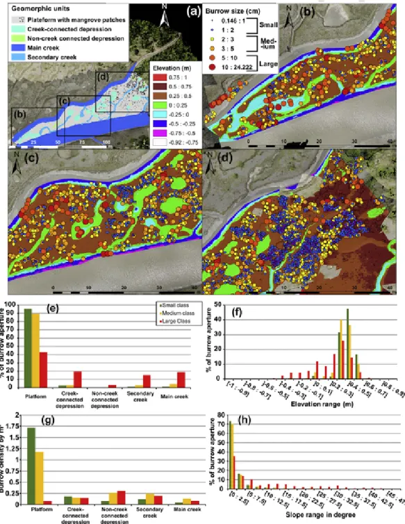
The three size classes of burrow apertures were visible throughout the study area but with variable abundance (Fig. 9). Small, medium and large size classes represented 55%, 39% and 6%, respectively, of the total number (i.e., 4459). The abundance of the S and M classes in-creased from SW to NE where the mudflat has a larger platform sur-face, is more elevated, and less incised by creeks and depressions. More than 90% of S and M class apertures were located on the platform, with

Fig. 9. Spatial distribution of crab burrow apertures for each size class (S: small; M: medium; L: large) over the study area: (a) overview of the area of interest; elevation (m) defined in

terms of three main zones: SW (b), central (c), and NE (d); burrow aperture sizes are in cm for each size class; (e) number of apertures (expressed in %) as a function of geomorphic units; (f) elevation range; (g) burrow density per m2_{for each geomorphic unit; and (h) mean surface slope.}

UNCORRECTED

PROOF

do not portray the heterogeneous distribution of these burrows. L class apertures were, in contrast, much more abundant on steep slopes (up to 30°) and on low-elevation features such as collapsing banks or bottoms of depressions. A large concentration of L apertures (60%) was associ-ated with connected creek banks, while unconnected depressions had a low proportion (5%). The L class density on these geomorphic units ranged from 0.15 to 0.3 apertures per m2_.

A more detailed scrutiny shows that >35% of apertures belonging to the S and M classes were located mostly over the nearly flat inner platform surface at an elevation of 0.3 to 0.5 m (Fig. 9) where slopes were >5°, whereas L class apertures occurred at elevations ranging from −0.4 m to 0.6 m, with a slight maximum around 0.3–0.4 m, and had a wide range of slopes of up to 35°.

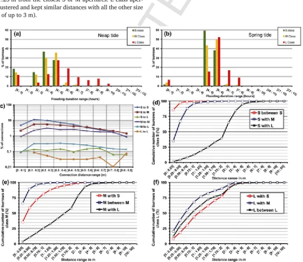
Differences in elevation induce variability in flooding duration of the crab burrows as a function of their location (Fig. 10). During neap tides, S and M burrow apertures were located where flooding duration was shortest (0 to 4 h). Only L class apertures were found in areas flooded >6 h. During spring tides, 90% of S and M apertures were located in areas flooded for 4–5 h, whereas L class apertures were found in areas with flooding durations of 4 to 8 h.

Fig. 10 depicts the spatial relationships between burrow aperture size classes from Delaunay connection edges used to define aperture spa-tial clusters. S and M apertures were nearest to each other and most clustered: 100% of the apertures in each of these classes were distant to each other by <75 cm and 1 m, respectively. Regarding the L class, they appeared as isolated features less related to other aperture classes, with 50% located >1.25 m from the closest S or M apertures. L class aper-tures were not clustered and kept similar distances with all the other size classes (distance of up to 3 m).

Using the tie distance between apertures yielded by Delaunay trian-gulation (Fig. 5), the structure of relationships between aperture size classes was assessed in terms of community clusters (Fig. 10). The dom-inant ties were S-connected with a 0.6 m maximum tie connection. The ties connecting the S class to M apertures are less abundant than the pre-vious tie relations. The tie relations with the L class are less represented than the others in community clusters.

Following Delaunay triangulation, we defined 194 burrow aperture community clusters over the study site (Fig. 11). The area of these clus-ters was very variable, ranging from 1.6 cm2_{for the smallest ones to 96} m2_{for the largest one. In this part of the workflow, averaged area and} derived statistic indexes were not used due to outliers such as very large clusters located in the E sector of the mudflat. In order to segment clus-ters as a function of their extension, three classes were defined using the minimum cluster area, the median, the third quartile and the maximum area: Class 1 - Small-sized clusters (S, minimum of 1.6 cm2_{to the median} of 0.1334 m2_{), Class 2 - Medium-sized clusters (M, from the median to} the third quartile of 0.5751 m2_{), and the Class 3 - Large-sized clusters (L,} from third quartile to maximum). In the 192 clusters determined, class 1 represented 50%, class 2 25% and class 3 25%. The burrow apertures composing these clusters were located mostly on the mudflat platform at a mean elevation range of 0.3 to 0.6 m and slope range of 0 to 15°.

The spatial distribution of S-sized clusters showed that they were mostly located in the SW part of the study site where the mud platform was narrow. These clusters included 2 to 10 burrow apertures. 90% of them included 2 to 5 apertures. These clusters were located at low ele-vations (<0.2 m) for around 20% of them, and 37% on steep surfaces

Fig. 10. Descriptive statistical indexes of burrow aperture environment and proximity: (a) percentage of burrow apertures as a function of flooding duration (hours) during neap tides; (b)

percentage of burrow apertures as a function of flooding duration (hours) during spring tides; (c-f) proximity indexes between burrow apertures for the different aperture classes created from the Delaunay triangulation.

UNCORRECTED

UNCORRECTED

PROOF

Fig. 11. Mapping of classes of burrow aperture community clusters (Small, area < 13.34 dm2_{; Medium, area > 13.34 dm}2_{< 57.51 dm}2_{; Large, area > 57.51 dm}2_{) and summary of their}

environmental characteristics: (a) overview of mudflat geomorphology; (b-d) parts of the area of interest with mapped surface facies classes and locations of the three different classes of burrow aperture community cluster; descriptive statistical indexes were calculated within each cluster as: (e) number of burrow apertures within clusters; (f) average elevation in m; and (g) average slope in degrees; average area (in %) of facies F1 to F4, summarizing the environmental parameters typically encountered for: (h) Small; (i) Medium; and (j) Large clusters. (>10° inclination). The average ratio of surface colour represented 9.1%

for F1, 25.9% for F2, 6.7% for F3, and 54.8% for F4.

Like the previous cluster class, the M-sized clusters were located in the SW and central parts of the study site. The number of apertures in each cluster ranged from 2 to 20, 70% of them having a range of 5 to 10. 80% of these clusters were located at elevations up of to 0.3 m and 96% on the platforms with a <15° inclination. The average ratio of surface colours represented 9.7% for F1, 32.8% for F2, 8.3% for F3, and 47.6% for F4.

The L-sized cluster classes were mostly located in the central and E parts of the study site where the platform exhibited large spaces between creeks and the depression network. This network clearly explains the fragmented distribution of these clusters. 68% of these clusters included a number of burrow apertures ranging from 10 to 50 and 16% from 50 to 200. Two very large and continuous clusters located on the E border of the study site included 500 to 1500 burrow apertures each. The aver-age ratio of surface colours represented 5.6% for F1, 25.4% for F2, 5.4% for F3, and 58.7% for F4.

4. Discussion

The discussion will focus on two themes: (a) the advantages offered by SfM photogrammetry for monitoring mudflat biogeomorphology, and (b) the contribution of the technique to a better understanding of mud-flat biogeomorphic processes.

4.1. Technical advantages and limits of UAV-based SfM photogrammetry for monitoring mudflat biogeomorphology and processes

SfM photogrammetry, especially based on UAV implementation, ap-pears as a ground-breaking technique for coastal studies in various fields related to the earth sciences (Brunier et al., 2016a; Casella et al., 2014; Gonçalves and Henriques, 2015; Jaud et al., 2016; Ander-son et al., 2019). UAVs offer cost advantages and survey adaptabil-ity and repeatabiladaptabil-ity that are lacking when manned airplanes are used for photogrammetric surveying. Coastal environmental studies can ben-efit fully from UAV-based photogrammetry by considering: (1) the large range of camera solutions available as payload and (2) the specific ca-pability of UAV platforms to fly at very low altitude, especially for stud-ies such as that reported here, which require very high-resolution re-mote sensing. The geomorphology of mudflats is particularly difficult to map using classic field survey methods (Anthony et al., 2008). UAV-based remote sensing further matches pretty well with the opera-tional aims of inter-disciplinary studies combining geomorphology and biology that require a spatial approach in deciphering visible processes, such as bioturbation, with accuracy and at a high resolution. The main shortcomings of the method highlighted in our study are: the drift of accuracy of the DSM outside the GCP coverage area, the need for nu-merous GCPs that are susceptible to perturb the mudflat morphology and biology, the water-logged or very wet surfaces which generated re-construction artefacts, and the time-consuming task of manual interpre-tation of surface feature extraction from orthophotographs, DSMs and derived products. Dropping-off GCPs is a serious issue in this type of study. GCPs are still needed for SfM photogrammetry but the GCP cov-erage bounds the accuracy of a DSM to a limited area, in this case to the mudflat area between two main creeks. Moreover, operator de-ployment of GCPs creates disturbances that include collapsing/obliter-ation of geomorphic features and burrow apertures, or footprints on the biofilm, not to mention the time-consuming and exhausting nature

of walking over a very unstable substrate. Recent developments in UAV positioning integrating RTK/PPK GPS solutions for image-georeferenc-ing and precise orientation with high-quality inertial measurement units can limit GCP problems in future studies by reducing the number of GCPs and by increasing the area of centimetre-range accuracy survey (Forlani et al., 2018; Taddia et al., 2019; Zhang et al., 2019). Surface moisture and the presence of water are also a serious issue for SfM photogrammetry on mudflats, especially when these are com-posed of fresh intertidal deposits. These conditions generate sun glint and relatively homogeneous textures which hinder, or induce bias in, the detection of tie points and alter dense picture correlation during photogrammetric processing. This creates artefacts such as over-esti-mated elevations or outliers. In such circumstances, one way of mitigat-ing these problems could consist in conductmitigat-ing surveys durmitigat-ing homoge-neous cloudy conditions in order to reduce the sun-glint effect. In our study, water-logged areas formed creeks and depressions. These were generally very narrow features that we excluded from the analysis. An-other issue, which is now relatively well resolved by the SfM photogram-metry workflow, is camera calibration. In the case of our survey, the GCP layout enabled Agisoft Photoscan modelling of intrinsic and extrin-sic camera parameters from the generic model. Integrated in most com-mercial and professional program solutions, auto-calibration processes enable the use of consumer-grade cameras.

Burrow aperture diameter mapping, which is one of the most im-portant outcomes of this study, was realised using manual extraction of features. This was a time-consuming task, especially without the help of an automatic aperture extraction method based on the shadow cast by an aperture. This could be done using deep-learning algorithms ap-plied to image features such as convolutional neural network (CNNs) algorithms (Hung et al., 2014; Vetrivel et al., 2018; Zeggada et al., 2017). The sediment colours facies, which corresponded here to the degree and the type of micro-algal development, were delimited on or-thophotographs. In order to avoid class confusion, supervised classifica-tion was limited to a number of colour classes, here four. The recent development of miniaturised global shutter matrix multispectral cam-eras or push-broom hyperspectral camcam-eras can help in the classification of mudflat surfaces based on spectral signatures and vegetation indexes such as the normalised difference vegetation index, and in the quantifi-cation of micro-algal development in terms of biomass. A combination of a sensor with very high spatial resolution in the visible spectrum and a sensor with a lower spatial resolution but more spectral bands should draw benefit from the advantages offered by both. Some of this equip-ment is now becoming available for UAV operations, but the quality is still inferior to that offered by manned aircraft which can embark heavy hyperspectral cameras (Launeau et al., 2018). Future work on mud-flat biogeomorphology needs to consider the possibility of embarking at least a multispectral camera in addition to the implementation of a clas-sical SfM photogrammetric survey with a standard RGB camera. 4.2. Contribution of SfM photogrammetry to the understanding of biogeomorphic processes on a tropical mudflat

The durations of the flooding tide over the mudflat associated with substrate elevation are key variables in the spatial structuring of thic activities (e.g., distribution of crab burrows and locations of ben-thic biofilms). Areas of lower elevation are flooded for longer periods, whatever the fortnightly tidal stage, and this influences the develop-ment of biofilms. As the substrate becomes more elevated, the shorter

UNCORRECTED

PROOF

crabs which prefer stabilised and drier sediments (Bertness and Miller, 1984). Our study has established, for the first time, the elevation thresh-old (0.25 m, equal to 4 to 5 h and 3 to 4 h of flooding for spring and neap tides respectively) at which these small mangrove crabs start bur-rowing. Aschenbroich et al. (2016) found that the crab community in pioneer mangroves in the study area was exclusively composed of Uca maracoani spp., the development of which is encouraged by contin-uous exposure to sunlight, and of juveniles of Uca spp. or Goniopsis cru-entata, thus indicating that pioneer mangrove environments may favour recruitment for juveniles. We also showed that the colour intensity of benthic biofilms strongly decreased in elevated substrates, notably plat-forms which exhibit the most abundant burrow apertures. This is espe-cially the case in the NE sector of the study area where the density of small and medium-sized apertures was higher than in the S sector. As-chenbroich et al. (2016) found a low Chl-a and high Phaeo:Chl-a ra-tio on the platform surface, reflecting impoverishment in labile organic matter due to grazing by U. cumulanta on the platform. The weak colour intensity of benthic biofilms on the generated orthophotographs was thus clearly attributable to the fiddler crabs feeding on the microphy-tobenthos (Ribeiro and Iribarne, 2011), and our UAV-based method has enabled 2-D mapping of biofilm distribution (F1 to F3) in relation to burrow aperture distribution at different substrate elevations, and dis-crimination by crabs foraging on biofilms based on the suitability or not of the latter for consumption.

Our study also showed that larger burrow apertures associated with bigger individuals are mostly established along channels or depressions, where substrate elevation decreases, but where steep edge slopes are still characterised by a dense biofilm, mainly visible as the dark green Facies 1. This may suggest that bigger crabs avoid this biofilm be-cause it may contain components that are not suitable for foraging (e.g., cyanophycae) or that such apertures do not belong to fiddler crabs because the steep microenvironment is too unstable for these crabs. Under these conditions, the preservation of these biofilms contributes to substrate stabilisation (Debenay et al., 2007; Lundkvist et al., 2007; Widdows et al., 2000). The significant logarithmic relation-ships between the percentage of burrow apertures and the mean slope brings out the absence of small and medium-sized apertures when such slopes are strongly inclined. Above an inclination of 10° the number of medium-sized and small apertures diminishes, whereas larger aper-tures can still subsist over slopes of up to 30° on the edges of channels and depressions. This suggests that the clustering patterns for small and medium-sized apertures are different from those of large apertures. The tie distance between apertures showed a strong proximity between small and medium-sized apertures (< 75 cm) whereas large apertures seem to be disconnected with the smallest ones (> 3 m). These results confirm the idea that crabs living in small and medium-sized burrows are bur-row-centred grazers in dense fiddler crab colonies, with an active space rarely exceeding 1 m2_{(Zeil and Hemmi, 2006), whereas individuals} inhabiting large burrows have a larger territory, implying competition for space rather than for food.

The high density of small and medium-sized burrow apertures on the platform is associated with more important sediment reworking, through excavation and grazing (pelletisation), by the small burrowers than that associated with the larger burrowers along channels and de-pressions (Aschenbroich et al., 2016), as suggested by the absence of excavation mounds and the presence of an intact biofilm. Such sed-iment reworking likely enhances substrate erosion, thus favouring the formation of incipient channels and depressions, as observed in salt marshes by Escapa et al. (2004, 2008) and Minkoff et al. (2006). The 2D mapping of crab burrow apertures yields a general overview of their spatial heterogeneity which is driven by the presence of geomor

phic habitats (platform, depressions and creeks). While the study of As-chenbroich et al. (2016) revealed strong spatial heterogeneity in pi-oneer mangroves because of the lack of replications (due to the diffi-cult field conditions), the UAV-based method employed in our study en-ables the visualisation and quantification of this spatial heterogeneity at a high resolution, thus providing new perspectives for the study of bio-geomorphic processes and ecosystem functioning at larger scales in dy-namic coastal environments.

5. Conclusion

The morphology of a mudflat surface and a number of its microben-thic characteristics have been mapped, and various morphometric as-pects quantified using SfM-based photogrammetry with input data from a UAV flying at low altitude. The technique combines the reproducibil-ity of traditional topographic surveys using RTK-DGPS or a total station and the high survey-point density and accuracy of LiDAR, but at much lower cost than the latter. The very fine scale of resolution brings out the significant potential of this method in the biogeomorphic character-isation of difficult and unstable environments such as a rapidly evolving mudflat. In addition to the fine scale of analysis, the method is non-in-trusive and of low-cost, fundamental advantages that favour repeated surveys to monitor patterns of mudflat evolution at various timescales (semi-diurnal tide, daily, neap-spring, seasonal). SfM photogrammetry thus not only can contribute to characterizing substrate geomorphol-ogy at the cm-scale but also to a better understanding of mudflat sur-face ecology and patchiness at this same fine scale. The method has en-abled precise quantification and determination of the spatial and tem-poral distribution of small-scale benthic aspects such as substrate fea-tures, notably developing networks of tide-water evacuation channels, their banks, and water-logged depressions that entail topographic diver-sity under pioneer mangroves, stages of biofilm development, and the sizes of crab burrow apertures. This quantitative approach is, in turn, a useful tool that should facilitate a better understanding of patterns of de-velopment of the mudflat substrate, and the role of bioturbation in sedi-ment mixing, biogeochemical cycles and the developsedi-ment and evolution of benthic food webs. Such fine-scale data can also be incorporated into data-fusion systems comprising data from other remote-sensing systems more adapted to larger-scale biogeomorphic applications (satellite im-ages and aerial photographs, multispectral and hyperspectral imagery, LiDAR and, of course, more conventional manned airborne photogram-metry), to address issues of spatial characterisation of the benthos and benthic ecological patchiness, and reliable sampling and upscaling. CRediT authorship contribution statement

Guillaume Brunier: Conceptualization, Methodology, Investigation, Formal analysis, Data curation, Writing - original draft, Writing - review & editing, Visualization. Emma Michaud: Conceptualization, Method-ology, Investigation, Formal analysis, Writing - original draft, Writing - review & editing, Supervision, Project administration, Funding ac-quisition. Jules Fleury: Conceptualization, Methodology, Investigation, Formal analysis, Data curation, Writing - original draft, Writing - re-view & editing. Edward J. Anthony: Formal analysis, Writing - origi-nal draft, Writing - review & editing, Funding acquisition. Sylvain Mor-van: Methodology, Investigation. Antoine Gardel: Methodology, Writ-ing - review & editWrit-ing, FundWrit-ing acquisition.

Declaration of competing interest

The authors declare that they have no known competing financial in-terests or personal relationships that could have appeared to influence the work reported in this paper.