Climatic reconstruction for the Younger Dryas/Early Holocene transition and the Little Ice Age based on paleo-extents of Argentière glacier (French Alps)

HAL Id: hal-03102778

https://hal.archives-ouvertes.fr/hal-03102778

HAL is a multi-disciplinary open access

archive for the deposit and dissemination of sci-entific research documents, whether they are pub-lished or not. The documents may come from teaching and research institutions in France or abroad, or from public or private research centers.

L’archive ouverte pluridisciplinaire HAL, est destinée au dépôt et à la diffusion de documents scientifiques de niveau recherche, publiés ou non, émanant des établissements d’enseignement et de recherche français ou étrangers, des laboratoires publics ou privés.

Climatic reconstruction for the Younger Dryas/Early

Holocene transition and the Little Ice Age based on

paleo-extents of Argentière glacier (French Alps)

Marie Protin, Irene Schimmelpfennig, Jean-louis Mugnier, Ludovic Ravanel,

Melaine Le Roy, Philip Deline, Vincent Favier, Jean-François Buoncristiani,

Team Aster, Didier Bourlès, et al.

To cite this version:

Marie Protin, Irene Schimmelpfennig, Jean-louis Mugnier, Ludovic Ravanel, Melaine Le Roy, et al.. Climatic reconstruction for the Younger Dryas/Early Holocene transition and the Little Ice Age based on paleo-extents of Argentière glacier (French Alps). Quaternary Science Reviews, Elsevier, 2019, 221, pp.105863. �10.1016/j.quascirev.2019.105863�. �hal-03102778�

Climatic reconstruction for the Younger Dryas/Early Holocene

1

transition and the Little Ice Age based on paleo-extents of

2

Argentière glacier (French Alps)

3

4

Marie Protina, Irene Schimmelpfenniga, Jean-Louis Mugnierb, Ludovic Ravanelc, Melaine Le 5

Royc, Philip Delinec, Vincent Favierd, Jean-François Buoncristianie, ASTER Teama 6

7

a

Aix-Marseille Univ, CNRS, IRD, INRA, Coll France, CEREGE, Aix-en-Provence, 13545, 8 France 9 b , CNRS, ISTerre, Chambéry, 10 73000, France 11 c , CNRS, EDYTEM, Chambéry, 12 73000, France 13 d

Université Grenoble Alpes, CNRS, IRD, Grenoble INP, IGE, Grenoble, France 14

e

Biogéosciences, UMR 6282 CNRS, Université Bourgogne Franche-Comté, 6 Boulevard 15

Gabriel, Dijon, 21000, France 16

17

, Karim Keddadouche) 18

19

Correspondence to: Marie Protin (protin@cerege.fr)

20

21

Abstract

22

Investigation of Holocene extents of mountain glaciers along with the related naturally-driven 23

climate conditions helps improve our understanding of glacier sensitivity to ongoing climate 24

change. Here, we present the first Holocene glacial chronology in the Mont-Blanc massif 25

(Argentière glacier) in the French Alps, based on 25 in situ-produced cosmogenic 10Be dates 26

of moraines and glacial bedrocks. The obtained ages from mapped sequences of moraines at 27

three locations reveal that the glacier was retreating from its Lateglacial extent and oscillating 28

several times between ~11.7 ka and ~10.4 ka, i.e. during the Younger Dryas/Early Holocene 29

(YD/EH) transition, before substantially retreating at ~10.4 ka. Climate conditions 30

corresponding to the past extents of Argentière glacier during the YD/EH transition (~ 11 ka) 31

and the Little Ice Age (LIA) were modelled with two different approaches: by determining 32

summer temperature differences from reconstructed ELA-rises and by using a Positive 33

Degree Day (PDD) mass-balance model coupled with a dynamic ice flow model. The ELA-34

rise reconstructions yield a possible range of summer temperatures for the YD/EH transition 35

that were cooler by between 3.0 and 4.8°C compared to the year 2008, depending on the 36

choice of the ELA sensitivity to summer temperature. The results from the PDD model 37

indicate temperatures cooler by ~3.6 to 5.5°C during the YD/EH transition than during the 38

1979-2002 period. For the LIA, our findings highlight that the role of local precipitation 39

changes, superimposed on the dominant temperature signal, is important in the detailed 40

evolution of the glacier. Overall, this study highlights the challenge that remains in accurately 41

inferring paleoclimate conditions from past glacier extents. 42

43

Keywords

44

Holocene; Glaciation; Western Europe; Cosmogenic nuclides; Glacier fluctuations; French 45

Alps; Moraine dating; Paleoclimate reconstruction; PDD modeling 46

47

1. Introduction

Investigating natural climate changes during the Holocene is relevant for assessing the impact 49

of the current climate changes, because Holocene climate variations were similar in amplitude 50

to the ones that are historically observed and predicted for the next few decades (e.g. Marcott 51

et al., 2013). Mountain glaciers are known to be sensitive climate change indicators 52

(Oerlemans, 2005), as their dynamics in the mid-latitudes, e.g. in the European Alps, depend 53

both on summer temperature and winter precipitation variations. They thus represent a highly 54

useful proxy for Holocene climate reconstructions. The ongoing trend of global glacier 55

retreat, which started after the end of the Little Ice Age (LIA), in the middle of the 19th 56

century, is well recorded with instrumental measurements (Leclercq et al., 2014). Evidence of 57

pre-instrumental glacier fluctuations are recorded by glacial landforms, which provide the 58

opportunity to reconstruct past glacier chronologies and examine glacier-climate interactions 59

over a longer period. In particular, moraine deposits give valuable information about past 60

glacier extents and dating them using in situ cosmogenic nuclides allows us to put glacier 61

variations into a spatio-chronological framework. Over the past few years, a growing number 62

of studies in the Alps have reported advanced glacier positions during the Late Glacial and 63

Holocene relying on in situ-produced cosmogenic beryllium-10 (10Be) moraine dating (e.g. 64

Moran et al., 2016; Schimmelpfennig et al., 2014; Schindelwig et al., 2012). In several of 65

these studies, the corresponding equilibrium line altitudes (ELA) were estimated (e.g. Baroni 66

et al., 2017; Hofmann et al., 2019; Le Roy et al., 2017). As the ELA directly depends on the 67

climate, in particular on atmospheric temperature and precipitation, reconstruction of past 68

ELAs provides the opportunity to estimate paleoclimate conditions. Atmospheric temperature 69

variations can be inferred using the adiabatic lapse rate or an ELA sensibility to atmospheric 70

temperature, as has previously been done in the Alps by Hofmann et al. (2019), Le Roy et al. 71

(2017) and Moran et al. (2016). However, this approach assumes that the impact of 72

precipitation on the glacier behavior is negligible or that the precipitation amount did not 73

change through time, potentially leading to a bias in the deduced temperature variations. In 74

the Alps, only few studies have attempted so far to infer precipitation changes from past 75

glacier extents (e.g. Keeler, 2015; Kerschner and Ivy-Ochs, 2007), as disentangling the 76

detailed contributions of both precipitation and temperature changes to glacier fluctuations is 77

still difficult (Solomina et al., 2016). 78

In this study, we explore the frontal and lateral moraines, as well as roches moutonnées 79

located beyond the limits of the LIA extent of Argentière glacier with the objective to present 80

the first alpine Holocene glacier chronology based on 10Be dating in the Mont-Blanc massif. 81

Potential climatic conditions corresponding to past extents of Argentière glacier are 82

determined using two different approaches, including a PDD mass-balance model, which 83

allows considering both precipitation and temperature variations. 84

85

2. Study site, geomorphologic setting and previous work on the past fluctuations of

86

Argentière glacier

87

45°55’N 6°57’ ) h h-western side of the Mont Blanc 88

massif, is the second largest glacier in the French Alps (Figure 1). In 2008, it covered a 89

surface of ~14 km2 with a length of almost 10 km and an altitude range spanning 3530 m to 90

1550 m a.s.l. (Six and Vincent, 2014; Vincent et al., 2009). Since 2009, the tongue (7 % of the 91

glacier area) is disconnected from the main glacier body and remains fed by an icefall located 92

at ~2200 m a.s.l. This tongue is covered by debris since at least the middle of the 20th century 93

(aerial photography from IGN, https://remonterletemps.ign.fr), while it was uncovered in the 94

middle of the 19th century according to pictorial documents from the LIA (Fontaine, 2015). 95

The ELA has been measured at ~2890 m a.s.l. between 1995 and 2011 (Six and Vincent, 96

2014). The mean annual temperature and precipitation were 6.5°C and 1238 mm in Chamonix 97

- Le Bouchet, the nearest weather station located at 1042 m a.s.l. for the time period 1961-98

1990 (Météo France) and are estimated at 1.8°C and 1783 mm at ~2000 m a.s.l. next to 99

Argentière glacier for the time period 1979-2002 (Joly et al., 2018 and personal 100

communication of D. Joly). Snow accumulation on the glacier at 3000 m a.s.l. is known to be 101

3 times larger than valley precipitation due to the orographic effect on precipitation, impact of 102

the wind and of avalanches, as the glacier is surrounded by steep slopes (Six and Vincent, 103

2014). Climatic data began to be collected in the Alpine region in the year 1760 (temperature 104

measurements) and in the year 1800 (precipitation) and are compiled in the HISTALP project 105

(http://www.zamg.ac.at/histalp/; Auer et al., 2007). 106

107

Figure 1 : General overview of the study area. (a) Location of the Mont Blanc massif (red

108

dot) in the Alps (red dotted line). (b) Landsat 8 image of the Mont Blanc massif from April

109

2005, with the 2008 extent of glaciers in blue. French glaciers: Gardent et al. (2014); Swiss

110

glaciers: Fischer et al. (2014); Italian glaciers: Smiraglia et al. (2015). Argentière glacier is

111

highlighted in dark blue. Red dotted lines represent countries borders. Red square represents

the location of Figure 2 and white squares represent the sampling locations, shown in Figure

113

7.

114

The Argentière glacier catchment is mainly formed by granite from the late Hercynian along 115

with Variscan metamorphic rocks (Bussy et al., 2000). Numerous preserved moraine ridges 116

and moraine remnants are visible in the catchment, close to the glacier, and downstream in the 117

Arve valley providing evidence of the past fluctuations of Argentière glacier (Figure 2). 118

While it’ h h LI w -known (Bless, 1984; Payot, 1884; Vincent et al., 119

2009), few chronological data constrain its Holocene fluctuations prior to the 17th century 120

(Bless, 1984; Le Roy, 2012). During the Last Glacial Maximum (LGM), the valleys around 121

the Mont Blanc massif were glacierized, and the glacier surface reached an altitude of 2400 m 122

a.s.l. at the location of Argentière glacier, as reconstructed from the trimline positions in the 123

region of the Mont Blanc massif (Figure 2, Coutterand and Buoncristiani, 2006). During the 124

Late-Glacial, glaciers located on the western flank of the Mont-Blanc massif were still 125

connected as one glacier named Arve glacier, extending in the Arve valley over a distance of 126

30 km, where numerous and mostly lateral moraine relicts attest to multiple glacier 127

fluctuations during that period (Coutterand and Nicoud, 2005). At one point during the retreat 128

from the large Late-Glacial glacier extents, Argentière glacier disconnected from its neighbors 129

Mer de Glace and Tour Glacier, which is revealed by two latero-frontal moraines sets near La 130

Joux et near Le Planet in the Arve valley (Figure 2). Due to the lack of direct dating methods,

131

20th century studies on past glacier fluctuations were often based on the comparison of ELA 132

depressions, geomorphic moraine characteristics, pollen analyses or limiting radiocarbon 133

dates to correlate moraines within regionally defined relative glacier chronologies like the 134

“ ” f h w y . . Maisch, 1981). Such relative dating 135

was applied to the extent of Le Tour and Argentière glaciers and several interpretations 136

suggest that these moraines were deposited during the Late-Glacial or Early Holocene (Jaillet 137

and Ballandras, 1999; Lucéna and Ballandras, 1999; Bless, 1984), although there is no 138

indication for an univocal correlation to the classical Swiss alpine nomenclature. Further 139

evidence of Argentière glacier variations during the Holocene are provided by Bless (1984) 140

and Le Roy (2012). Radiocarbon dating of subfossil organic material found in stratigraphic 141

position in the right-lateral composite moraine (yellow dot on Figure 2) gave evidence of five 142

glacier advances between ~4 ka and 1.2 ka, i.e. during the so-called Neoglacial, a period when 143

the climatic conditions became more suitable for glacial advances (Bless, 1984). In the same 144

moraine profile, dating of detrital wood embedded-in-till 30 years later, indicates an advance 145

during the 9th century, similar in elevation to the LIA maxima (Le Roy, 2012). Finally, 146

Argentière glacier reached its LIA frontal maximum extent during the 17th century, according 147

to several written reports about the destruction or menace of villages by the advancing glacier 148

(Bless, 1984). 149

150

Figure 2 : Geomorphic map of the study area with individual sample locations on the 5 m

151

IGN DEM RGE ALTI. The 2008 extent of Argentière and nearby glaciers are represented in

blue (Gardent et al., 2014). Geomorphologic features were mapped based on Bless (1984)

153

and Le Roy (2012), DEM interpretation and field observations. Dashed lines represent

154

undated moraines, their ages are presumed from their position relative to moraines of known

155

ages; grey lines are moraines attributed to nearby glaciers.

156 157 3. Methodology 158 3.1. Moraine mapping 159

The geomorphologic map presented in Figure 2 was produced using Geographic Information 160

System (GIS). It is based on field observations along with interpretation of recent aerial 161

images (from the IGN, 50 cm resolution) and LIDAR digital elevation models (DEM), with 162

resolution of 1 m (Arve valley) and 2 m (Argentière catchment). The map in Figure 2 also 163

includes moraines that were mapped in earlier studies (Le Roy, 2012; Bless, 1984). 164

3.2. Sampling and cosmogenic 10Be ages

165

All samples were obtained using a cordless angle grinder, chisel and hammer (Figure 3). 166

Boulder samples were collected from the top of boulders embedded in the crests or on the 167

slopes of selected moraines and bedrock samples were preferentially taken from sloping 168

surfaces to minimize the risk of cover by vegetation, sediment or snow (Figure 3). We only 169

sampled surfaces with minimal signs of erosion, exhibiting glacial striation when possible, 170

and moraine boulders that were big enough (>1 m) to avoid the risk of exhumation. In total, 171

20 moraine boulders and 5 bedrock samples were collected. Topographic shielding was 172

determined in the field using a clinometer. 173

The chemical procedure for 10Be extraction from the rock was conducted at CEREGE (Aix-174

en-Provence, France). Samples were crushed and sieved to the 250-500 µm fraction. Quartz 175

was isolated from other grains first by magnetic separation, then either by repeated leaching 176

in a H2SiF6/HCl mixture or by froth flotation, and finally by at least three sequential leaching

177

steps in concentrated HF to remove remaining feldspar grains and atmospheric 10Be. About 178

0.1 g of a 3025 ± 9 ppm in-house 9Be carrier solution (Merchel et al., 2008) was added to the 179

purified quartz before its complete dissolution in concentrated HF. Beryllium was extracted 180

and purified by separation on anion and cation columns and by successive alkaline 181

precipitations of Be(OH)2, and the samples were then oxidized for one hour at 700°C. The

182

final BeO oxides were mixed with Nb powder and loaded into nickel cathodes for AMS 183

measurements. The 10Be/9Be ratios of all samples were measured at the French national AMS 184

facility ASTER (Arnold et al., 2010) and calibrated against in-house standard STD-11 with an 185

assigned 10Be/9Be ratio of (1.191 ± 0.013) x 10-11 (Braucher et al., 2015) using the 10Be half-186

life of (1.387 ± 0.0012) x 106 years (Chmeleff et al., 2010; Korschinek et al., 2010). 187

Analytical uncertainties due to AMS measurement include ASTER counting statistics and 188

stability (~0.5 %; Arnold et al. (2010)) and blank correction. Correction for the chemical 189

blanks, whose 10Be/9Be ratios range between (3.21 ± 0.50) x 10-15 and (4.87 ± 0.63) x 10-15, 190

were performed by subtracting their numbers of atoms 10Be from those of the samples 191

calculated from the 10Be/9Be ratios (Table 1). 192

193

Figure 3 : Photographs of sample sites at Argentière glacier. Example of (a) moraine boulder

194

(ARG-16-7), (b) inter-morainic bedrock surface and (c) roche moutonnée (ARG-15-6) along

195

with (d) roche moutonnée surface (ARG-15-5) sample from Lognan area. View of dated

196

moraines (e) L2 and (f) L3 (framed by the dashed line) located in the left-lateral Lognan area.

197

Surface exposure ages were calculated with the CREp online calculator (Martin et al., 2017) 198

applying the Lal-Stone time corrected scaling scheme, the ERA40 Atmosphere model and the 199

Atmospheric 10Be-based VDM for geomagnetic database (see Martin et al. (2017) and 200

f h ). h “ ” 10

Be production rate of 4.11 ± 0.10 atoms 10Be/g 201

established by Claude et al. (2014) was retained here as it is the only available regional 202

production rate. In addition, it yields results very similar to the NENA production rate (Balco 203

et al., 2009), which has often been used in previous studies in the Alps and has a value of 4.10 204

± 0.17 atoms 10Be/g when recalculated in CREp with the above parameters. We note that the 205

“ ” (Young et al., 2013; 4.12 ± 0.25 atoms 10

Be/g according to CREp), 206

also used for several alpine studies, would lead to ages younger by ~ 0.25 %. Calculated 207

exposure ages are presented in Table 1. We did not correct the ages for snow cover effects or 208

surface erosion, as these effects were minimized by sampling boulders least likely to have 209

been snow covered and with minimal signs of erosion. Applying a high snow cover correction 210

corresponding to 50 cm of snow for 6 months, as used in Chenet et al. (2016), would lead to 211

y ≤ 8 % and assuming an erosion rate of 1 mm.kyr-1

(André, 2002) would lead to 212

ages older by only 1%. Nonetheless, the presented ages should be considered minimum 213

exposure ages. 214

3.3. Glacier reconstruction and paleoclimatic modelling

215

Two approaches were used to infer paleoclimatic conditions from the extents of Argentière 216

glacier. Both approaches are based on the simplified assumption that the glacier is in 217

equilibrium with the climate conditions during the respective present-day reference periods 218

detailed below. 219

3.3.1. GIS-based ELA reconstruction and paleo-temperature determination

220

In the first approach, 3D glacier surface reconstructions were generated for different glacier 221

extents in the past using the ArcGIS toolbox GlaRe (Pellitero et al., 2016) based on the 222

mapping of the moraines presented in Figure 2. The topography of the bedrock beneath of 223

Argentière glacier used for the reconstruction was determined by subtracting the ice thickness 224

(Rabatel et al., 2018) from the 25 m IGN DEM BD Alti. ELA calculations were then done 225

using the ArcGIS toolbox developed by Pellitero et al. (2015) according to the Area-Altitude 226

Balance Ratio (AABR) with a balance ratio of 1.59 and the Accumulation Area Ratio (AAR) 227

method with a ratio of 0.67, both values representative for the Alps (Pellitero et al., 2015; 228

Rea, 2009). While the AAR methods is simply based on the ratio between the surface of the 229

accumulation area and the surface of the entire glacier, the AABR method take into account 230

the hypsometry of the glacier (Osmaston, 2005) and the mass balance gradient (Benn and 231

Lehmkuhl, 2000) and is therefore considered more reliable to approximate ELAs (Lukas, 232

2007; Pellitero et al., 2015). However, the AAR method has most often been used in the Alps 233

(e.g. Hofmann et al., 2019; Le Roy et al., 2017; Moran et al., 2016). Thus, for the 234

paleoclimatic discussion we prefer the results inferred from the ELAs calculated with the 235

AABR method and the results from the AAR method are only used for the sake of 236

comparison with other Alpine sites. We adjusted the shear stress value along the flowlines in 237

the ArcGIS toolbox GlaRe (Pellitero et al., 2016) by comparing the ELA calculated for the 238

2008 extent of Argentière glacier to the mean ELA measured in the field between 1995 and 239

2011 (∼2890 m, Six and Vincent, 2014). The best estimate are found for a shear stress value 240

of 150 kPa and an automatic shape factor. The calculated ELAs for the 2008 extent are 2866 241

m using the AABR method and 2801 m using the AAR method. These two values are close, 242

yet inferior, to the measured ELA. It has to be noted that in 2008 the glacier was not in 243

steady-state, therefore the measured ELA does not reflect an equilibrium position unlike the 244

calculated values, which hinders us from accurately fitting both and might explain the 245

difference between them. 246

The difference of the resulting paleo-ELAs between two periods allows for determination of 247

the associated variation in atmospheric temperature (T) by using a constant ELA sensitivity to 248

atmospheric temperature (S) and assuming the same precipitation as today, following the 249

q Δ = Δ L / . The ELA sensitivity to summer temperature is nonetheless difficult 250

to estimate and two values are used in this paper: 115 m°C-1, which is relevant for French 251

Alpine glaciers (Rabatel et al., 2013); and 72 m°C-1, which was empirically quantified for 252

Argentière glacier by Six and Vincent (2014) and takes into account the local effects of 253

temperature and all meteorological parameters that influenced the snow and ice ablation. 254

255

Figure 4 : Climatic data of Argentière glacier between 1979 and 2002 at ∼ 2000 m a.s.l.. Blue

256

bars represent the cumulated monthly precipitation, the blue and red curves represent

257

respectively the minimum and maximum monthly temperatures. 1 to 12 represents the months

258

January to December.

259

3.3.2 PDD modelling

260

In the second approach, combinations of precipitation and temperature variations and ELAs 261

for different glacier extents were determined by using a PDD mass-balance model coupled 262

with a dynamic ice flow model, described in Blard et al. (2007). This model has previously 263

been used for glaciers in the central pacific by Blard et al. (2007), in the Andes by Jomelli et 264

al. (2011) and in Greenland by Biette et al. (2018). The topography of the watershed of 265

Argentière glacier used for the modeling is the same used for the GIS-based reconstructions 266

(see section 3.3.1.). The model was calibrated using the mass-balance data from 1979 to 2002 267

(considered here as the present-day reference period) collected at Argentière glacier by the 268

GlacioClim Network (https://glacioclim.osug.fr) from extensive field measurements on 10 269

markers distributed along the glacier (5 in the ablation area and 5 in the accumulation area) 270

and local monthly values of temperature and precipitation for the same period (personal 271

communication of D. Joly), inferred at 2000 m a.s.l. in the Argentière catchment from a 272

downscaling method based on a geomatic spatial model (Joly et al., 2018). Figure 4 depicts 273

the monthly values of temperature and precipitation of Argentière glacier averaged from 1979 274

to 2002 as used in the model. This interval is nearly twice as long as the 10-14 years response 275

time of the glacier front position to a mass balance change (Vincent et al., 2009) and is long 276

enough to fade out the inter-annual variability. In addition, the glacier length at the beginning 277

of this period is very similar to that at the end, as it includes an advance of the glacier 278

followed by an equal retreat (Figure 5). This consolidates the assumption that the glacier was 279

roughly in equilibrium with the mean climatic condition during this period. This period is put 280

into a broader context and compared to the variations of Argentière glacier since 1800 in 281

Figure 5. The atmospheric lapse rate of temperature and precipitation are fixed at 0.65°C/m 282

and 80mm/100m/year, respectively. This precipitation lapse rate matches best the field data 283

taking into the range of the precipitation lapse rate between precipitation in the valley and at 284

high altitude in the MMB of 52mm/100m/years (Corbel, 1963) as well as the variable ratio 285

between valley precipitation and winter accumulation on Argentière glacier (Six and Vincent, 286

2014) equivalent to a lapse rate of ∼95mm/100m/years. 287

288

Figure 5 : (a) Annual temperature anomalies (reference period 1979-2002); (b) annual

289

precipitation in the west part of the Alps from the HISTALP time series (Auer et al., 2007)

290

and (c) front variation of the Argentière glacier - the origin of the axis is arbitrary

(1818-291

1880: Payot, 1884 in Fontaine, 2015; 1850: Bless (1984); 1880-2000: Francou and Vincent,

292

2007; > 2000: Vincent et al., 2009. Red and blue curves represent 10-years running means.

293

Period of reference of the climatic data of Argentière glacier (1979-2002) used as input in the

294

PDD model is highlighted in green. Periods considered for extracting the temperature values

295

for the 1820 and 1850 glacier extents, accounting for the glacier’s response time, are

296

highlighted in purple and pink, respectively. The extracted mean temperatures are depicted by

297

white horizontal lines.

298

Figure 6 shows the correlation between observed and calculated mass balance of Argentière 299

glacier. This best fit (R2 = 0.97) was obtained using the least mean square optimization on the 300

determination of the melting factor (MF) used in the PDD model, whose values are MFsnow =

301

2.3 mm w.e. °C-1 d-1 and MFice = 5.1 mm w.e. °C-1 d-1. These values are close to the ones

defined in Réveillet et al. (2017) for Argentière glacier: MFsnow = 3.5 mm w.e. °C-1 d-1 and

303

MFice = 5.5 mm w.e. °C-1 d-1. Using these parameters and the climatic inputs presented in

304

Figure 4, the calculated ELA is 2940 m a.s.l., whereas Argentière glacier ELA measurements 305

using satellite images during the years 1984 to 2002 ranged between 2623 and 2861 m a.s.l. 306

(Rabatel et al., 2013). Furthermore, the length of the modeled glacier is between 600 and 300 307

m shorter than that of Argentière glacier between 1990 and 2001. As the lower part of the 308

Argentière glacier is covered by debris from before the middle of the 20th century, and termini 309

of debris-covered glaciers, like the Miage glacier in the Mont Blanc massif (Smiraglia et al., 310

2010), are often less responsive to climatic variability than non-covered glaciers (Scherler et 311

al., 2011), this might be the reason why the model predicts a shorter length. Nonetheless, due 312

to the excellent agreement between calculated and measured mass balance (Figure 6), we 313

consider that the above calibration of the model is suited for modeling the past extents of the 314

glacier. For each investigated extent, the model considers all potential combinations of 315

precipitation and temperature conditions that lead to a match of the front of the modeled 316

paleo-glacier with the position of the corresponding frontal moraine mapped in the field. 317

ELAs correspond to the altitudes where the glacier mass balance is zero. For each glacier 318

extent, ELAs vary over a range of more than 100 m, due to the large range of assumed 319

precipitation conditions (between 0 and 2 times that of the reference period). 320

321

Figure 6: (a) Comparison between observed mass balance (1979-2002; Glacioclim Network)

322

on the Argentière glacier (blue dotes) and mass balance calculated by the PDD model (red

323

curve). (b) Comparison between the modelled glacier extent for the reference period of

1979-324

2002 (red dotted line), the 2001 extent (blue dotted line; Le Roy, 2012) and the 2008 extent

325

(blue area; Gardent et al., 2014).

326

327

4. Results

328

4.1. Description of the geomorphological evidence

329

Figure 2 presents a moraine map of the Argentière catchment. The frontal moraines located 330

around 1.5-2 km downstream of the present glacier front (purple moraines in Figure 2) have 331

been assigned by Bless (1984) to four LIA advances between the 17th century and 1850 based 332

on analysis of historical written documents and paintings combined with lichenometry dating. 333

On both lateral sides, the LIA advances are represented by massive composite moraines of up 334

80 h h ≥ 1 k h. e between the ~1850 frontal 335

moraine and the current front, representing the generally gradual retreat of the glacier since 336

the end of the LIA (pink moraines in Figure 2). Immediately to the north, slightly outboard of 337

the right-lateral LIA composite moraine, four short ridges of so far unknown age are 338

preserved (orange moraines in Figure 2). This area, hereafter calle “Crèmerie”, is covered by 339

a dense conifer forest, but the morphology of the ridges is noticeable on the DEM and attested 340

by a few disseminated moraine boulders. 341

Further upstream near the present-day Argentière glacier icefall, multiple ridges of lateral 342

moraines are preserved. On the left-lateral side, in the “Lognan” h 343

prominent moraine, ~15 m-high and 700 m-long is attributed to the LIA (Figure 2). Only a 344

few tens of meters outboard, two dissected main ridges and several subridges lie tight together 345

(among them L2 and L3 in Figure 2), and another dissected ridge is preserved about 150-200 346

m further outboard (L1 in Figure 2). According to their positions, these ridges are pre-LIA 347

moraine relicts but were undated until now. They display a smoother morphology than the 348

massive LIA moraine, but are located around the same altitude, and exhibit several boulders 349

suitable for sampling. At their upstream (southern) ends, these moraines abut against a steep 350

and up to a 150 m-high bedrock outcrop, which testifies to past glacial cover owing to 351

numerous roches moutonnées (Figure 3). This roche moutonnée area lies between the current 352

terminus of Rognons glacier and the left-lateral bank of Argentière glacier and is framed by 353

two moraines deposited by Rognons glacier during its retreat. A similar moraine sequence 354

pattern is observed on the north-eastern bank of the glacier. Moraines located further to the 355

west of the pre-LIA deposits in the Lognan area (grey moraines on Figure 2) are not 356

considered as moraines built by Argentière glacier. They were most likely deposited by the 357

Lognan glacier, a smaller nearby glacier. This is suggested by their composition of gneiss 358

boulders, transported from the Lognan glacier catchment, whereas the boulders embedded in 359

the sampled moraines are granitic according to the main lithology of the Argentière glacier 360

catchment. 361

Downstream in the Arve valley near La Joux, relicts of a latero-frontal moraine set are 362

preserved (dark blue moraines in Figure 2). These moraines, smooth and covered by conifer 363

trees, were studied and mapped in detail by Bless (1984) and Lucéna and Ballandras (1999) 364

“L h ff II” “L J x” (Lucéna and Ballandras, 1999), corresponding to 365

J1 and J2 moraines respectively in Figure 2. Furthermore, remnant of at least one other 366

moraine is located between J1 and J2. Some boulders are embedded in these moraines. A set 367

of lateral ridges are observed along the right-lateral valley flanks on the NW side of the 368

Argentière glacier catchment, especially south of Le Planet. North of these moraines, another 369

set of latero-frontal moraine relicts deposited by the neighbor Tour Glacier are visible near Le 370

Planet (Figure 2).

371

4.2. Moraine and bedrock exposure ages

372

All 10Be exposure ages are listed in Table 1 and depicted in Figure 7. In the text, individual 373

exposure ages are presented with their 1 analytical errors; in addition, Table 1 shows the 1

374

external errors, including the 10Be production rate error. Before calculating the mean ages of 375

the glacial landforms, each age population was subject to a 2 test (2 ) to identify any 376

potential outliers. The landform ages correspond to the arithmetic means of the sample ages 377

and the uncertainties to their standard deviations (in the text and figures for internal 378

comparison); Table 1 also shows the errors that include the 10Be production rate errors. 379

Probability plots of all boulder and moraine mean ages are illustrated in Figure 8. 380

Five samples from La Joux area yield ages between 13.2 ± 0.4 ka (LJX-17-5), corresponding 381

to an isolated boulder in front of the outmost moraine (J1), and 9.7 ± 0.3 ka (LJX-17-4), 382

which is the only age from J1 moraine. The mean age for the J2 moraine is 10.9 ± 0.9 ka (n = 383

2), after discarding sample LJX-17-1 (51.9 ± 2.7 ka) as an outlier. This latter boulder surface 384

was most likely affected by isotope inheritance from earlier periods of exposure to cosmic 385

radiation. Ages for the J1 and J2 frontal moraines are not in stratigraphic order, but the J1 age 386

relies upon only one sample, which might have been underestimated due to surface cover by 387

vegetation, erosion or anthropogenic impact, as the La Joux area is located in an area covered 388

by forest, close to a village. 389

Sample name Latitude (dd) Longitude (dd) Altitude (masl) Thickness (mm) Shielding factor Quartz weight (g) Carrier (mg 9Be) Associated blank 10_Be/9_Be x10-14 [10Be] (x 104 at.g-1) 10_{Be age} (ka) 1 analytical error (ka) 1 external error (ka) LOGNAN AREA MORAINE SAMPLE L1 11.66 ± 0.70 (0.76) ARG-16-9 45.96670 6.96065 2252 26 0.939 26.18 0.2979 30Jan17 35.8 ± 1.7 26.8 ± 1.3 12.21 0.58 0.64

ARG-16-10 (O) 45.96680 6.96056 2246 32 0.939 27.08 0.2996 30Jan17 29.9 ± 2.0 21.8 ± 1.5 10.10 0.64 0.68

ARG-16-11 45.96691 6.96050 2239 25 0.950 28.16 0.3008 30Jan17 33.0 ± 1.4 23.3 ± 1.0 10.63 0.42 0.48 ARG-16-12 45.96704 6.96041 2235 40 0.949 28.08 0.3062 30Jan17 35.8 ± 2.1 25.8 ± 1.5 11.88 0.68 0.73 ARG-16-13 45.96744 6.96031 2216 38 0.959 27.79 0.3012 30Jan17 36.1 ± 1.7 25.8 ± 1.2 11.93 0.55 0.61 L2 10.44 ± 0.19 (0.32) ARG-16-1 45.96575 6.96317 2287 20 0.970 27.84 0.2996 30Jan17 33.6 ± 2.2 23.8 ± 1.6 10.28 0.66 0.70 ARG-16-2 45.96575 6.96320 2274 50 0.970 27.55 0.2995 30Jan17 32.5 ± 2.1 23.3 ± 1.5 10.39 0.65 0.69 ARG-15-11 45.96551 6.96333 2265 45 0.969 12.75 0.3063 9Mai16 15.27 ± 0.47 23.87 ± 0.77 10.65 0.32 0.40 L3 10.41 ± 0.37 (0.45) ARG-16-3 45.96641 6.96312 2255 27 0.973 26.99 0.2993 30Jan17 32.9 ± 1.1 24.03 ± 0.79 10.61 0.33 0.41 ARG-16-4 45.96648 6.96289 2247 35 0.98 26.44 0.2993 30Jan17 31.7 ± 1.0 23.66 ± 0.77 10.52 0.32 0.40 ARG-15-12 45.96686 6.963 2235 22 0.974 18.27 0.3058 9Mai16 22.3 ± 0.7 24.41 ± 0.77 10.87 0.33 0.40

ARG-16-5 (O) 45.96703 6.96292 2234 20 0.971 27.98 0.3019 30Jan17 55.8 ± 5.0 39.9 ± 3.6 17.42 1.49 1.55 ARG-16-6 45.96736 6.96278 2216 50 0.971 28.00 0.3001 30Jan17 30.60 ± 0.95 21.60 ± 0.68 10.04 0.30 0.38 ARG-16-7 45.9679 6.96246 2189 30 0.971 28.63 0.3005 30Jan17 31.1 ± 1.1 21.50 ± 0.77 10.01 0.34 0.41 BEDROCK SAMPLE ARG-15-5 45.96075 6.96705 2502 30 0.978 18.49 0.312 9Mai16 26.56 ± 0.96 29.6 ± 1.1 11.02 0.37 0.45 ARG-15-6 45.96123 6.96753 2465 20 0.977 9.37 0.3083 9Mai16 15.41 ± 0.57 33.2 ± 1.2 12.50 0.45 0.54 ARG-15-7 45.96181 6.96773 2427 35 0.974 8.09 0.3047 9Mai16 11.42 ± 0.41 27.9 ± 1.0 11.02 0.38 0.46 ARG-16-8 45.96650 6.96061 2384 25 0.485 13.25 0.2965 3Avril17 8.93 ± 0.46 12.86 ± 0.70 10.44 0.53 0.58 ARG-16-14 45.96727 6.96208 2252 28 0.969 20.20 0.2985 3Avril17 22.94 ± 0.96 22.3 ± 1.0 9.97 0.40 0.46 CREMERIE AREA C1 ARG-17-1 (D) 45.98111 6.93959 1396 22 0.954 19.71 0.3009 3Avril17 1.79 ± 0.21 1.36 ± 0.22 1.16 0.19 0.21 ARG-17-2 45.98112 6.93975 1399 28 0.952 19.76 0.2903 3Avril17 1.55 ± 0.15 1.07 ± 0.16 0.90 0.14 0.14 ARG-17-3 (D) 45.98099 6.93985 1403 22 0.954 20.54 0.2817 3Avril17 1.65 ± 0.28 1.07 ± 0.26 0.89 0.23 0.23 C2 ARG-17-4 (D) 45.98070 6.93989 1407 36 0.960 20.16 0.2983 3Avril17 2.8 ± 3.3 2.32 ± 0.33 2.04 0.31 0.31 ARG-17-5 (D) 45.98046 6.94044 1408 28 0.956 20.47 0.2515 3Avril17 4.98 ± 0.47 3.64 ± 0.39 3.24 0.34 0.35 LA JOUX AREA

J2 10.93 ± 0.86 (0.90) LJX-17-1 (O) 45.96437 6.90778 1214 24 0.955 12.01 0.2993 15Jan18 33.2 ± 1.6 54.7 ± 2.6 51.93 2.67 2.98 LJX-17-2 45.96380 6.90743 1216 32 0.955 15.45 0.3091 15Jan18 8.28 ± 0.52 10.61 ± 0.69 10.32 0.64 0.68 LJX-17-3 45.96318 6.90777 1213 41 0.955 23.66 0.3067 15Jan18 13.99 ± 0.53 11.82 ± 0.46 11.53 0.43 0.51 J1 LJX-17-4 45.96231 6.90604 1215 28 0.955 20.23 0.3007 15Jan18 10.41 ± 0.32 9.99 ± 0.32 9.70 0.30 0.38 LJX-17-5 45.96139 6.90607 1209 48 0.955 21.63 0.3083 15Jan18 14.41 ± 0.45 13.4 ± 4.3 13.17 0.41 0.52 Carrier 10_Be/9_{Be x10}-14 10_Be

BLANKS (mg 9Be) (x 104 at)

9Mai16 0.3068 0.321 ± 0.046 6.6 ± 1.0 30Jan17 0.3002 0.452 ± 0.057 9.1 ± 1.2 3Avril17 0.2788 0.487 ± 0.073 9.1 ± 1.4 15Jan18 0.3075 0.348 ± 0.050 7.2 ± 1.0

Table 1: Sample [A] and blanks [B] details, analytical data related to 10Be measurements and surface exposure ages. Outliers (O) were

determined based on 2 test (2 ). Mean landform ages are also indicated with standard deviations and total uncertainties in parentheses. Samples from the Crèmerie area have been discarded (D) as the current were <1µA and blank corrections >50%.

391

Figure 7: Individual 10Be exposure ages (white boxes) and mean 10Be ages (colored boxes) of

392

glacial landforms (moraines and glacially polished bedrock) in the study areas of the

393

Argentière glacier (a) La Joux, (b) Crèmerie, and (c) Lognan. Red dots represent bedrock

394

samples and green dots boulder samples. Outliers, rejected based on 2 statistics, are in italic

395

grey font. Errors of individual ages correspond to the analytical error only. Mean ages are

396

arithmetic means and standard deviation.

397

In the Lognan area, the three bedrock samples taken from roches moutonnées slope between 398

Rognons glacier and Argentière glacier yield ages of 11.0 ± 0.4 (ARG-15-7), 12.5 ± 0.5 399

(ARG-15-6) and 11.0 ± 0.4 ka (ARG-15-5). From the moraine sequence located directly to 400

the north, we dated three moraines (L1-L3), two of which lie very close together (L2, L3; 401

Figure 7) The outmost one (L1) yields five boulder ages between 12.2 ± 0.6 and 10.6 ± 0.4 402

ka, with a mean of 11.7 ± 0.7 ka, after discarding ARG-16-10 (10.1 ± 0.6 ka) as an outlier. 403

Three boulders were dated from L2, giving ages between 10.3 ± 0.7 and 10.7 ± 0.3 ka and a 404

mean age of 10.4 ± 0.2 ka. L3 yields five ages between 10.0 ± 0.3 and 10.9 ± 0.3 ka with a 405

mean age of 10.4 ± 0.4 ka, after removing ARG-16-5 (17.4 ± 1.5 ka) as an outlier. These 406

glacial landform ages are in good stratigraphic order. The similar 10Be ages of the latero-407

frontal moraines in the La Joux area (between ~10.9 ka and 9.7 ka) and of the lateral moraines 408

in the Lognan area (between ~11.7 ka and 10.4 ka) implies that the deposition of these 409

moraines most likely corresponds to the same glacier advances or stillstands. 410

411

Figure 8 : Summed probability plots (colored curves – colors refer to the legend of Figure 2)

412

of 10Be boulder ages from Argentière glacier. Probability curves of individual ages (black

413

curves) include analytical errors only. Ages indicated in each box are arithmetic means and

414

standard deviations, also visually represented as vertical lines and colored band. Grey curves

415

are outliers.

416

Two additional bedrock surfaces were sampled next to the Lognan moraines. One on the foot 417

of the bedrock slope at the southern extremity of L1 was dated at 10.4 ± 0.5 ka (ARG-16-8), 418

and another one located between L1 and L3, taken from the flat ground, was dated at 10.0 ± 419

0.4 ka (ARG-16-14). Even if these two ages are statistically indistinguishable from the mean 420

ages of the moraines that framed them and the low number of bedrock ages does not allow a 421

robust comparison, they apparently tend to be slightly younger than the moraines. This could 422

be explained by degradation and erosion of the samples (in the case of ARG-16-8) and 423

sediment, vegetation and/or snow cover, in particular for ARG-16-14 as it is on ground level, 424

which in both cases results in an underestimation of the ages. 425

The batch of the five samples taken in the Crèmerie area (C1 and C2 moraines) was subject to 426

a failure during the chemical preparation of the samples, leading to low-quality 427

measurements. Only sample ARG-17-2 from moraine C1 was retained due to sufficiently 428

high 9Be currents (>1 µA) during the AMS measurements, and yielded an age of 0.9 ± 0.2 ka. 429

However, as this is only a single moraine age with high analytical error and therefore does not 430

allow us to reliably interpret the deposition age of the moraines in the Crèmerie area, we do 431

not consider it further. 432

Based on presented ages and on the mapping of all preserved moraines, we reconstruct the 433

extents of the glacier during the YD/EH transition and the Little Ice Age maximum in 434

comparison with that of the year 2008, as shown in Figure 9. 435

436

Figure 9 : Black curves represent the reconstruction of past extents of the Argentière glacier,

437

based on mapping of the preserved moraines and interpretation of 10Be dating, for the (A)

438

Younger Dryas/Early Holocene transition (~11 ka - J2 moraines) (B) LIA maximum (17th

439

century) and (C) year 2008. Dashed glacier limits with “?” correspond to hypothetical

440

extents. Blue extensions represent the vertical projection of the 3D reconstruction with the

441

ArcGIS toolbox GlaRe.

442

4.3. ELA determination

443

The ELAs resulting from the different methods described in section 3.2 are presented in Table 444

2. The contours of the ice surface resulting from the 3D reconstructions using the ArcGIS 445

toolbox GlaRe and used for the ELAs calculations are represented in Figure 9 (blue areas). 446

According to the GIS-based reconstruction method, the ELAs computed for the glacier extent 447

corresponding to the LIA maximum (17th century) and the moraine J2 (∼11 ka) using the 448

AABR method are 2738 m and 2523 m a.s.l., respectively. With the AAR method, they are 449

2753 m and 2648 m a.s.l., respectively. The ELA rise between the two extents is of 215 m 450

with the AABR method, while it is 105 m with the AAR method. The modeling of the same 451

extents using the PDD model, assuming the same precipitation as today, leads to ELA values 452

of 2753 m for the 17th century and 2442 m a.s.l. for the ~11 ka period. The associated ELA 453

rise between the two extents is 311 m. 454

ELA (m a.s.l.) ΔELA (m)

present LIA ~11 ka

(J2 moraine) LIA - present ~11 ka - present 11 ka - LIA

AABR 2866 2738 2523 128 343 215

AAR 2801 2753 2648 48 153 105

PDD 2940 2753 2442 187 498 311

Table 2: Comparison of ELA calculations using the AABR and AAR methods and the PDD

455

modeling for Argentière glacier for the present-day (i.e. year 2008 for the AABR and AAR

456

methods and 1979-2002 for the PDD modeling), the LIA maximum (17th century) and the J2

457

moraine (~11 ka; YD/EH transition). For the AABR method a Balance ratio of 1.59 (Rea,

458

2009) is used and for the AAR method a ratio of 0.67 (Gross et al., 1977), both representative

459

for the Alps. For the PDD model, ELA values are inferred with the same precipitation

460

condition as today.

461

4.4. Paleoclimatic results

462

4.4.1. Temperature results from the GIS-based reconstructions

463

The temperature differences inferred from the GIS-based ELA reconstructions (AABR and 464

AAR methods) between ~11 ka, the LIA maximum (17th century) and the year 2008 are 465

presented in Table 3. The 128-m rise of the ELA between the LIA maximum and the year 466

2008 inferred from the AABR method is equivalent to a +1.1°C difference in summer 467

temperature, according to the ELA sensitivity to summer temperature of 115 m°C-1 (Rabatel 468

et al., 2013). Using the local ELA sensitivity of 72 m°C-1 (Six and Vincent, 2014), it is 469

+1.8°C. The temperature difference between ~11 ka and the year 2008 (ELA-rise of 331 m), 470

using the same two ELA temperature-sensitivity values as above, is +3°C and +4.8°C, 471

respectively. 472

For the sake of comparison with other studies from the Alps, we also give the results from the 473

AAR method, noting that the ELA-rise is traditionally estimated with reference to the LIA 474

maximum glacier extent. According to this approach, our reconstruction leads to an ELA-rise 475

between ~11 ka and the LIA maximum of 105 m, which corresponds to +0.9°C and +1.4°C, 476

respectively. Between ~11 ka and 2008, this approach gives a difference of +1.3°C and 477

+2.1°C, respectively, equivalent to an ELA rise of 153 m. And between the LIA maximum 478

and 2008, the ELA-rise is 48 m, corresponding to a temperature difference of +0.4°C and 479

+0.7°C, respectively. These latter results seem to be underestimated when comparing them to 480

the values inferred from the measurements at the beginning of the 19th century (~+1.0°C; 481

Auer et al., 2007; Figure 5), a period when the glacier was even slightly smaller than during 482

the 17th century. On the other hand, the temperature results from the AABR method 483

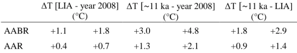
(+1.1°C/+1.8°C) are coherent with the instrumental data. 484 Δ [LIA - year 2008] (°C) Δ [~11 ka - year 2008] (°C) Δ [~11 ka - LIA] (°C) AABR +1.1 +1.8 +3.0 +4.8 +1.8 +2.9 AAR +0.4 +0.7 +1.3 +2.1 +0.9 +1.4

Table 3: Comparison of the temperature differences inferred from the ΔELA calculated from

485

the AABR and AAR methods (presented in Table 2) using two different ELA sensitivity to

486

temperature: 115 m°C-1 (Rabatel et al., 2013) on the left and 72 m°C-1 (Six and Vincent,

487

2014) on the right. LIA refers to the LIA maximum (17th century).

488

4.4.2. Paleoclimatic results from the PDD modeling

489

Applying the PDD modeling approach, we determined the potential combinations of 490

precipitation and temperature conditions corresponding to each investigated glacier extent. 491

The glacier extents at four different dates were investigated (see Figure 2 to visualize the 492

extents): the years 1850 and 1820, for which the glacier extents and regional climate 493

conditions are well known, the 17th century (LIA maximum) and the extent at ~11 ka using 494

the moraine J2 as the frontal limit. The modeling gives an infinite number of combinations of 495

temperature and precipitation conditions that explain the frontal moraine position at the four 496

investigated dates. The curves in Figure 10 represent these combinations, considering 497

temperatures between 0°C and 8°C below that of the reference period (1979-2002) and 498

precipitation amounts between 0 and 2 times that of the reference period. This figure also 499

shows the range of ELAs resulting from the model for each of the four glacier extents. The 500

ELAs increase with precipitation. 501

502

Figure 10 : Paleoclimatic reconstructions of the Argentière glacier for the YD/EH transition

503

(blue) and the 17th century (orange), 1820 (purple) and 1850. (pink) glacier extent.

504

Temperature changes, with respect to the 1979-2002 period, are plotted against relative

505

precipitation amount normalized to the 1979-2002 period. One curve reflects all

506

combinations of temperature and precipitation for one glacier extent (constrained by the

507

frontal moraines). The altitudes refer to the ELA associated with each

temperature-508

precipitation couple.

Climate influence on Argentière glacier is explored through modeling of its extents at the end 510

of the LIA, when climatic evolution is already instrumentally recorded. As the instrumental 511

climatic data used for comparison with our results do not cover the 17th century, only the 512

results of 1850 and 1820 are subject to discussions of the LIA paleoclimate. Based on the data 513

collected in the HISTALP project (http://www.zamg.ac.at/histalp/; Auer et al., 2007), we 514

estimate the annual temperature for the years 1850 and 1820. We then deduce the 515

precipitation, which is more likely to vary locally, from the PDD model. All values are 516

calculated relative to the 1979-2002 wh h h “ - y” f iod used 517

in the PDD model (see section 3.2). A shift of 10-14 years between the extraction of the 518

temperature value and the date of the studied extent has been applied in order to take into 519

account the ’ response time (Vincent et al., 2009). The measured temperature 520

differences compared to the period of reference are around -1.4°C for 1850 and around -1.0°C 521

for 1820 (Figure 5). Thus, colder conditions prevailed when the glacier was shorter, in 1850. 522

According to these temperature differences and the temperature-precipitation relationships in 523

Figure 11, precipitation amounts were lower by ~15% in 1850 and higher by ~10% in 1820 524

compared to the 1979-2002 average. If the temperatures had been inferred from our PDD 525

model assuming the same amount of precipitation as in 1979-2002, the 1850 temperature 526

would have been overestimated by ~0.4°C and the 1820 temperature underestimated by 527

~0.2°C. 528

Constraining a unique temperature/precipitation couple for the ~11 ka glacier extent is much 529

more challenging due to the scarcity and uncertainties of pure precipitation and paleo-530

temperature records for this time in the Alps. Therefore, we use the following rationales to 531

narrow down the potential range of precipitation/temperature couples. As moraines are only 532

built below the ELA (e.g. Anderson and Anderson, 2010) and the maximal elevation of the 533

moraine sequence corresponding to the YD/EH transition on the glacier bank opposite to the 534

Lognan area is ~2400 m a.s.l. (Figure 2), the ELA during this period was at least as high as 535

2400 m. This observation allows us to limit the temperature difference compared to 1979-536

2002 to -5.5°C (lower bound) and to a minimum of 45% of the 1979-2002 averaged 537

precipitation amount (Figure 10 and Figure 11). Then, assuming that the amount of 538

precipitation was not superior to that during the end of the LIA, i.e. up to 10% precipitation 539

more than during the 1979-2002 period, the upper temperature limit is at -3.6°C. The 540

temperature values of -3°C and -4.8°C, inferred above from the GIS based estimations 541

(AABR method) for the same glacier extent, compare well with these temperature bounds of -542

5.5°C and -3.6°C resulting from the PDD model, supporting the findings from both methods. 543

The relatively high potential temperature ranges reflect the uncertainty arising from the choice 544

of the value for the ELA sensitivity to temperature in the first approach and from the range of 545

possible precipitation amounts in the second approach. 546

547

Figure 11 : Same as Fig. 10, but for the YD/EH transition (blue), 1820 (purple) and 1850

548

(pink) glacier extent only, with marks of the paleoclimatic interpretations.

549

550

5 Discussion

5.1. Holocene oscillations of Argentière glacier

552

As outlined in section 2, numerous glacio-geomorphic markers in the Arve valley attest to the 553

glacier extents during the LGM and to various advances or stillstands during the deglaciation 554

of the Late-glacial. The moraine ages from the La Joux and Lognan areas are younger than 555

11.7 ka and therefore fall into the Early Holocene, apart from L1 moraine, which overlaps 556

with the Younger Dryas within uncertainties. The 10Be ages of the three roche moutonnée 557

samples located between Rognons and Argentière glacier (11.0 ± 0.4 ka, 12.5 ± 0.4 ka, 11.0 ± 558

0.4 ka) and of the Lognan bedrock surfaces (10.4 ± 0.5 ka and 10.0 ± 0.4 ka) suggest that the 559

general deglaciation of this area occurred during the YD/EH transition. These ages are 560

statistically the same as the 10Be mean ages of moraines L1, L2 and L3 (11.7 ± 0.7 ka, 10.4 ± 561

0.2 ka and 10.4 ± 0.4 ka) in the Lognan area, indicating that the deglaciation process was 562

shortly interrupted by glacier stillstands or re-advances. The isolated bloc dated at 13.2 ± 0.4 563

ka in front of the J1 moraine in the La Joux area tentatively suggests that the front of the 564

glacier may already have retreated to a similar position as moraines J1 and J2 ~2 ka before the 565

YD/EH transition, but this scenario would need more evidence to be confirmed. The existence 566

of at least five morainic ridges between L1 and L3 (Figure 7C) indicate that Argentière 567

glacier stagnated or re-advanced at least five times between ~11.7 and ~10.4 ka ago. These 568

results from the lateral moraines in the Lognan area are coherent with the observations in the 569

frontal area of La Joux, where at least three preserved ridges of Early Holocene age (~11 ka) 570

can be distinguished (among them J1 and J2). The similarity of the moraine and bedrock ages 571

as well as the smooth and low morphology of the moraines suggest that the glacier did not 572

retreat far up-valley between the moments of moraine deposition and that these moraines 573

correspond to periods of glacier stillstands during the deglaciation rather than to massive re-574

advances. Finally, the innermost moraine ages and the bedrock ages in the Lognan area imply 575

that the glacier definitively retreated from its Early Holocene extent at ~10.4 ka ago. 576

Further evidence of advanced extents of Argentière glacier during the Late Holocene comes 577

from the study by Bless (1984) who suggested five advances of Argentière glacier between ~4 578

ka and ~1.2 ka, based on radiocarbon-dated subfossil wood found in the right-lateral moraine 579

outcrop (location in Figure 2). Multiple advances during this period were also reported for 580

other glaciers in the Mont-Blanc massif (e.g. Deline and Orombelli, 2005; Le Roy et al., 581

2015). In particular, the numerous dendrochronologically-dated advances of the neighbor Mer 582

de Glace between ~3.5 ka and 0.7 ka ago (Le Roy et al. (2015); location in Figure 1), support 583

the hypothesis of Late Holocene advances of Argentière glacier. However, considering that so 584

far none of the preserved and dated moraines gave a Late Holocene age that pre-dates the 585

LIA, we assume that the Late Holocene extents of Argentière glacier were smaller than those 586

during the LIA maximum. 587

5.2. Paleoclimatic interpretations

588

5.2.1. Comparison with previously glacier-derived paleoclimate reconstructions from

589

Argentière glacier and other sites in the Alps

590

The results of the PDD modeling for the 1820 and 1850 extents indicate that precipitation was 591

higher in 1820 than in 1850. Regionally higher precipitation in 1820 was also recorded in the 592

western part of the Alps according to the HISTALP annual precipitation time series (Figure 593

5), but the difference in precipitation amount between 1850 and 1820 is only of ~10%, against 594

~20% according to our modeling. Our results are consistent with the conclusions from 595

previous PDD modeling of Argentière glacier (Vincent et al., 2005), which explains observed 596

glacier advances during the period 1760-1830 with winter precipitations higher by at least 597

25% than the 20th century average, while summer temperature had not decreased. They also 598

attribute the subsequent retreat of the glacier to a decrease in winter precipitation. Even if our 599

findings are not directly comparable, as our modelling only allows us to consider the annual 600

and not the seasonal climate variations and Vincent et al. (2005) based their model on less 601

cooling than we do here, we can still notice that the trend is the same, i.e. higher precipitation 602

in 1820 compared to 1850 explains the bigger glacier extent. Given that the 19th century 603

maximum of bigger glaciers in the Swiss Alps occurred in 1850-1860 rather than in 1820 604

(Holzhauser et al., 2005), the glacier size and local variations in precipitations during the LIA 605

could explain the detailed differences in the behavior of Argentière glacier compared to 606

smaller glaciers in other Alpine regions. These results illustrate that ignoring the role of 607

precipitation might lead to a first-order approximation of past temperature conditions. Our 608

results also show that the impact of local precipitation variations on mountain glacier 609

dynamics superimposes on those of large scale temperature variations and can thus explain 610

the local differences in the behavior of glaciers from different parts of a massif, like the Alps, 611

and the small fluctuations of a glacier during one glacial stadial, like the LIA. 612

Temperature reconstructions for the YD/EH transition using the AAR method have 613

previously been performed at glacier sites in the Alps. Moran et al. (2016) reconstructed from 614

the extents of two glaciers in the Eastern Alps that summer temperatures were 1.5°C lower 615

during the YD/EH transition than in the mid 20th century, which is in good agreement with the 616

difference of 1.3°C/2.1°C inferred from the extents of Argentière glacier during the YD/EH 617

transition and the year 2008 when using the AAR method. These results are also coherent 618

with the findings of Hofmann et al. (2019) who inferred a temperature difference of 1.5°C 619

between the YD/EH transition and the LIA in the westernmost French Alps. Nonetheless, due 620

to the extremely simplified assumptions on the glacier geometry of the AAR method (section 621

3.3.1), we believe that temperature reconstructions based on this approach should be taken 622

with caution. The coherence between the relative temperature reconstructed from the local 623

LIA maximum glacier extent and the one measured at the end of the LIA (section 4.4.1) 624

makes us indeed confident that the AABR method is more reliable than the AAR method 625

when inferring paleotemperatures from ELA reconstructions. 626

5.2.2. Comparison with paleoclimate results from independent proxy records

627

Comparison of our precipitation range assumptions for the YD/EH transition (-45% to +10% 628

of the present precipitation amount) with independent proxy records is difficult. Given that 629

precipitation can significantly vary locally, it would be ideal to consider a local precipitation 630

estimate in or near the Mont-Blanc massif for this period. However, to our knowledge this 631

does not exist. The complexity of the precipitation variability during the Younger Dryas and 632

the Early Holocene has indeed been underlined by Magny et al. (2001). Recent global climate 633

simulations combined with proxy-based temperature reconstructions suggest that the Younger 634

Dryas was considerably drier and the Early Holocene was less dry in Central Europe than the 635

preceding Allerod period (Renssen et al., 2018), but no quantification of the precipitation 636

conditions relative to the present is available. 637

Alpine and European temperature reconstructions for the Younger Dryas and Early Holocene 638

based on independent proxies are more frequent. However, the range of reconstructed annual 639

and summer temperatures for the Younger Dryas is large, it varies from 6 to 2°C below 640

modern values when inferred from records of pollen and cladocera assemblages from 641

Gerzensee in the North-alpine foreland in Switzerland (Lotter et al., 2000), investigation of 642

stalagmites in Hölloch cave in the German Alps (Wurth et al., 2004) or chironomid records 643

from a paleolake in the Central Swiss Alps (Ilyashuk et al., 2009). Based on high-resolution 644

oxygen isotope records, the beginning of the Holocene is associated with an abrupt 645

temperature rise on regional and hemispheric scale (Alley, 2000; Schwander et al., 2000). 646

Early Holocene temperature reconstructions in the region of the Alps yield, similar to those 647

for the Younger Dryas, a large range of values depending on the used proxy. For example, the 648

chironomid record in the Swiss central Alps indicates ~1-4°C above the present July air 649

temperatures for the very beginning of the Holocene (Ilyashuk et al., 2009), while a second 650

chironomid record, also from the Swiss Alps, indicates ~1-1.5°C below it (Heiri et al., 2003). 651