Sensitivity analysis of prior model probabilities and the value of prior knowledge in the 1
assessment of conceptual model uncertainty in groundwater modelling 2
3
Rodrigo Rojasa*, Luc Feyenb, Alain Dassarguesa,c 4
5 6
* Corresponding author 7
a Applied geology and mineralogy, Department of Earth and Environmental Sciences, 8
Katholieke Universiteit Leuven 9
Celestijnenlaan 200 E, B-3001 Heverlee, Belgium 10
Tel.: +32 016 326449; fax: +32 016 326401. 11
E-mail address: Rodrigo.RojasMujica@geo.kuleuven.be 12
13
b European Commission - DG Joint Research Centre (JRC), Institute for Environment and 14
Sustainability, Land management and natural hazards unit 15
TP261, Via E. Fermi 2749, 21027 Ispra (Va), Italy 16
Tel.: +39 0332 789258; fax: +39 0332 786653 17
E-mail address: luc.feyen@jrc.it 18
19
c Hydrogeology and environmental geology, Department of Architecture, Geology, 20
Environment, and Constructions (ArGEnCo), Université de Liège 21
B.52/3 Sart-Tilman, B-4000 Liège, Belgium 22
Tel.: +32 4 3662376; fax: +32 4 3669520 23
E-mail address: alain.dassargues@geo.kuleuven.be 24
Abstract 1
A key point in the application of multi-model Bayesian averaging techniques to assess the 2
predictive uncertainty in groundwater modelling applications is the definition of prior model 3
probabilities, which reflect the prior perception about the plausibility of alternative models. In 4
this article we analyze the influence of prior knowledge and prior model probabilities on 5
posterior model probabilities, multi-model predictions and conceptual model uncertainty 6
estimations. The sensitivity to prior model probabilities is assessed using an extensive 7
numerical analysis in which the prior probability space of a set of plausible 8
conceptualizations is discretised to obtain a large ensemble of possible combinations of prior 9
model probabilities. Additionally, we assess the value of prior knowledge about alternative 10
models in reducing conceptual model uncertainty by considering three example knowledge 11
states, expressed as quantitative relations among the alternative models. A constrained 12
maximum entropy approach is used to find the set of prior model probabilities that 13
correspond to the different prior knowledge states. For illustrative purposes, we employ a 3-14
dimensional hypothetical setup approximated by 7 alternative conceptual models. Results 15
show that posterior model probabilities, leading moments of the predictive distributions and 16
estimations of conceptual model uncertainty are very sensitive to prior model probabilities, 17
indicating the relevance of selecting proper prior probabilities. Additionally, including proper 18
prior knowledge improves the predictive performance of the multi-model approach, 19
expressed by reductions of the multi-model prediction variances up to 60%. However, the 20
ratio between-model to total variance does not substantially decrease. This suggests that the 21
contribution of conceptual model uncertainty to the total variance can not be further reduced 22
based only on prior knowledge about the plausibility of alternative models. These results 23
advocate including proper prior knowledge about alternative conceptualizations in 24
combination with extra conditioning data to further reduce conceptual model uncertainty in 25
groundwater modelling predictions. 26
Keywords 1
Multi-model prediction, uncertainty assessment, maximum entropy, prior knowledge, 2
conceptual model uncertainty 3
1. Introduction and scope 1
Groundwater modelling has become an essential part of groundwater management and 2
accurate model predictions are required to ensure an acceptable degree of confidence in 3
model results. However, incomplete knowledge about the geological setting and scarce or 4
prone to error information about model parameters, boundary conditions and input data, 5
render the predictions of groundwater dynamics and pollutant transport uncertain. Practice, 6
on the other hand, suggests that once a conceptual model is successfully calibrated its results 7
are rarely questioned and the conceptual model is assumed to be correct (Bredehoeft, 2005; 8
Hojberg and Refsgaard, 2005). However, a successful calibration does not guarantee the 9
correctness of the conceptual model. Rather, many parameter sets together with different 10
conceptual models may produce equally good results in a calibration process (Bredehoeft, 11
2003; Harrar et al., 2003; Carrera et al., 2005). In this sense, relying on a single hydrological 12
concept will likely produce biased and under-dispersive predictions due to neglecting 13
conceptual model uncertainty (Neuman, 2003). 14
15
In recent years, a number of multi-model methods have been proposed to address the problem 16
of conceptual model uncertainty in hydrological modelling (Neuman, 2003; Poeter and 17
Anderson, 2005, Ajami et al., 2005; Refsgaard et al., 2006). These methods seek to obtain 18
consensus predictions from a set of plausible models by linearly combining individual model 19
predictions. One such approach is Bayesian Model Averaging (BMA) (Draper, 1995; Hoeting 20
et al., 1999), which weights the predictions of competing models by their corresponding
21
posterior model probability, representing each model’s relative skill to reproduce system 22
behaviour in the training period. Hence, BMA weights are tied directly to individual model 23
performance. Several studies applying the method to a range of different problems have 24
demonstrated that BMA produces more accurate and reliable predictions than other existing 25
multi-model techniques (e.g., Raftery and Zheng, 2003; Ye et al., 2004; Ajami et al., 2005). 26
In the field of groundwater hydrology, applications of BMA have been rare. Neuman (2003) 1
proposed the Maximum Likelihood Bayesian Model Averaging (MLBMA) method, which is 2
an approximation of BMA that relies on maximum likelihood parameter estimation and 3
expanding around these values through Monte Carlo simulation. Ye et al., (2004) expanded 4
upon the theoretical framework of MLBMA and applied it to model the log permeability in 5
unsaturated fractured tuff using alternative variogram models. 6
7
Rojas et al., (2008) proposed a methodology to assess uncertainty in predictions of 8
groundwater models arising from errors in the model structure, forcing data and parameter 9
estimates by integrating the Generalized Likelihood Uncertainty Estimation (GLUE) (Beven 10
and Binley, 1992) methodology with BMA. The methodology is based on the concept that 11
there exist many good simulators of the system that may be located in different regions of the 12
combined model, input and parameter space, given the data at hand. For a set of plausible 13
system conceptualizations, input and parameter realizations are sampled from the joint prior 14
input and parameter space. A likelihood measure is then calculated for each simulator based 15
on its ability to reproduce system state variable observations. The integrated likelihood of 16
each conceptual model is obtained by integrating the likelihood of the different simulators 17
over the input and parameter space. The integrated likelihoods are consequently used in BMA 18
to weight the model predictions to obtain ensemble predictions. Key advantages of this 19
methodology are that: (i) there is no restriction on the diversity of conceptual models or on 20
the level of uncertainty in the input data or parameters that can be included; (ii) it does not 21
rely on a single optimum set of (calibrated) parameter values, hence, avoiding biased 22
parameter estimates that compensate for errors in model structure, input data and 23
measurement errors; (iii) it allows for different ways of expressing the likelihood of a 24
simulator (including a formal Bayesian one), hence allowing different types of knowledge to 25
be incorporated (quantitative as well as qualitative); and (iv) it is Bayesian in nature, which 26
provides a formal framework to incorporate prior knowledge about the model structures and 1
parameters, or to update the estimates should new information become available. 2
3
Rojas et al., (2008) applied the methodology by considering 7 alternative conceptualizations 4
with increasing complexity to represent a 3-dimensional synthetic example consisting of 2 5
aquifers separated by an aquitard. An extensive numerical analysis showed that neglecting 6
conceptual model uncertainty results in biased and overly conservative predictions. However, 7
two important aspects concerning the application of the methodology remained unanswered; 8
first, the sensitivity of posterior model probabilities, multi-model groundwater predictions, 9
and conceptual model uncertainty estimations to different sets of prior model probabilities; 10
and, second, the value of prior knowledge about the alternative conceptualizations to further 11
reduce conceptual model uncertainty. We address these two points in this article. 12
13
In Bayesian inference two basic interpretations can be given to prior probability distributions. 14
First, in the population interpretation, a prior distribution represents a population of possible 15
parameter values from which a potential candidate is to be drawn. Second, in the more 16
subjective state of knowledge interpretation, the guiding principle is that knowledge (and 17
uncertainty) about a given parameter must be expressed as if the value of that parameter 18
could be thought of as a random realization from the prior probability distribution (Gelman et 19
al., 2004, p. 39), i.e., prior probability distributions can be interpreted as a formal
20
representation of knowledge (uncertainty) about a given parameter. More importantly, there 21
is no unique prior probability distribution for representing this knowledge (uncertainty) (Kass 22
and Wasserman, 1996). 23
24
In Bayesian literature, different methods to assign prior probability distributions to different 25
classes of problems can be found. We do not wish to provide a complete overview of these 26
methods but refer the reader to Kass and Wasserman (1996) for an excellent review. 27
A key point when adopting a prior probability distribution is the influence of this distribution, 1
after updating, on the results. Two general courses of action can be mentioned to alleviate 2
this influence. First, with increasing data availability, prior probability distributions are 3
expected to have less influence on inferences about parameters and predicted variables (Kass 4
and Wasserman, 1996). Thus, one strategy consists in collecting as much data as possible to 5
overcome the influence of the prior probability distributions. For most groundwater 6
modelling applications, however, obtaining enough data to overrule the effects of prior model 7
probabilities may in many cases be cost prohibitive. Second, one can assign non-informative 8
prior probability distributions, with the uniform distribution being the most common case, 9
hoping that information contained in the data will dominate the form of the resulting posterior 10
distribution. Consequently, reported multi-model methodologies used in groundwater 11
modelling have employed, generally, a uniform prior model probability distribution reflecting 12
no prior preference on the plausibility of alternative conceptual models (see, e.g., Meyer et 13
al., 2007). This is also the approach followed by Rojas et al., (2008).
14 15
Panels of experts, prior elicitation, and theoretical or empirical grounds, on the other hand, 16
can be helpful in defining suitable prior model probabilities based on expert knowledge (see, 17
e.g., Ye et al., 2006). These prior model probabilities are inherently subjective, i.e., they 18
reflect preference over a particular conceptualization and, probably, other group of experts 19
will arrive to different prior model probabilities based on different grounds. In this context, 20
we stick to the idea expressed by Ghosh et al., (2006, p. 55) who stated that whenever prior 21
information is available, an attempt to use a prior probability distribution reflecting that prior 22
knowledge should be used as far as possible. 23
24
Given that there is no unique way to express the prior knowledge about alternative conceptual 25
models, due mainly to the subjective nature of the task, a procedure to select among potential 26
sets of prior model probabilities is required. Ye et al., (2005) recently proposed an approach 27
aimed to find a set of prior model probabilities that maximizes Shannon’s entropy (Shannon, 1
1948) subject to a series of constraints. Hereby, the constraints reflect prior knowledge about 2
the alternative conceptualizations. The key idea behind this approach is that uncertainty 3
represents “potential information” in the sense that when a random variable takes on a value 4
we gain information and lose uncertainty (Applebaum, 1996). In this sense, Shannon’s 5
entropy measures the amount of information contained in the set of prior model probabilities. 6
Therefore, less informative sets will have a higher entropy compared with more informative 7
sets since a larger amount of information can be gained in the first. For example, when the set 8
of prior model probabilities corresponds to the uniform prior distribution, i.e., all alternative 9
conceptual models have equal prior probabilities, we are at a state of maximum uncertainty 10
and entropy is at its maximum. When a more informative set of prior model probabilities is 11
available the entropy will be lower. 12
13
In the case that several sets of constraints reflecting different prior knowledge about the 14
conceptual models are proposed, the problem translates into a min-max choice, i.e., to find 15
the set of prior model probabilities that maximizes Shannon’s entropy subject to the 16
respective constraints, but which is minimum among different proposed sets. Solving this 17
min-max problem, however, does not guarantee optimum predictive performance. To 18
overcome this problem, Ye et al., (2005) propose to follow one of the following two 19
approaches: (1) when enough data are available to perform a meaningful model 20
(cross)validation, they advocate selecting a posteriori the set that outperforms based on 21
suitable performance criteria (see, e.g., Liang et al., 2001 for examples on performance 22
criteria); (2) when there is not enough data available to estimate meaningful posterior 23
measures of model quality, they advocate selecting the min-max set that, additionally, 24
maximizes the likelihood for the ensemble of alternative conceptual models. 25
In this work, we conduct a numerical experiment to analyze the sensitivity of the posterior 1
model probabilities, the groundwater multi-model predictions, and the conceptual model 2
uncertainty estimations to prior model probabilities. To this end, the prior probability space 3
of the alternative conceptual models is discretised in equidistant intervals and all possible 4
combinations of prior model probabilities for the set of conceptualizations are formed, given 5
that the sum of the prior model probabilities for each combination equals 1. 6
7
Furthermore, we extend upon the work of Ye et al., (2005) and assess the value of prior 8
knowledge about the plausibility of alternative conceptualizations in reducing conceptual 9
model uncertainty. To this end we employ the constrained maximum entropy approach 10
proposing (out of the ensemble of discrete sets of prior model probabilities) three sets of prior 11
model probabilities that reflect the following knowledge states: (i) a non-informative case 12
about the plausibility of alternative conceptualizations, i.e., alternative conceptual models 13
have equal prior probabilities; (ii) relevant and proper prior knowledge about the plausibility 14
of alternative conceptualizations, i.e., alternative conceptual models receive higher prior 15
probabilities as they approach a “true” 3-dimensional hypothetical setup; and (iii) improper 16
prior knowledge about the plausibility of alternative conceptualizations, i.e., alternative 17
conceptual models receive prior probabilities that are inconsistent as they approach the “true” 18
3-dimensional hypothetical setup. Results obtained using the three optimized sets of prior 19
model probabilities are compared to find the set that outperforms in terms of predictive 20
capacity and to assess the value of this prior knowledge to further reduce conceptual model 21
uncertainty. 22
23
The remainder of this paper is organized as follows. In section 2, we provide a condensed 24
overview of the combined GLUE-BMA methodology. Section 3 details a 3-dimensional 25
hypothetical aquifer system that is used to illustrate the methodology and to assess the 26
sensitivity of the groundwater multi-model predictions. Implementation details are described 27
in section 4. In this section, we elaborate on the different conceptual models, input and 1
parameter uncertainty, the methodology to account for the sensitivity of the results due to 2
different discrete sets of prior model probabilities and the constrained maximum entropy 3
method to assess suitable sets of prior model probabilities in agreement with prior 4
knowledge. Results are discussed in section 5 and a summary of conclusions is presented in 5
section 6. 6
7
2. Materials and Methods 8
To render the article self-contained sections 2.1 and 2.2 elaborate on the basis of GLUE and 9
BMA methodologies, respectively. For a detailed description the reader is referred to Rojas et 10
al., (2008).
11 12
2.1. Generalized Likelihood Uncertainty Estimation (GLUE) methodology 13
GLUE is a Monte Carlo simulation technique based on the concept of equifinality (Beven and 14
Freer, 2001). It rejects the idea of a single correct representation of a system in favour of 15
many acceptable system representations (Beven, 2005). For each potential system simulator, 16
sampled from a prior set of possible system representations, a likelihood measure is 17
calculated which reflects its ability to simulate the system responses, given the available 18
training data D. Simulators that perform below a subjectively defined rejection criterion are 19
discarded from the further analysis and likelihood measures of retained simulators are 20
rescaled so as to render the cumulative likelihood equal to 1. Ensemble predictions are based 21
on the predictions of the retained set of simulators, weighted by their respective rescaled 22
likelihood. 23
24
Likelihood measures used in GLUE must be seen in a much wider sense than the formal 25
likelihood functions used in traditional statistical estimation theory (Binley and Beven, 2003). 26
These likelihoods are a measure of the ability of a simulator to reproduce a given set of 27
training data, therefore, they represent an expression of belief in the predictions of that 1
particular simulator rather than a formal definition of probability. However, GLUE is fully 2
coherent with a formal Bayesian approach when the use of a classical likelihood function is 3
justifiable (see, e.g., Romanowicz et al., 1994). 4
5
In the work of Rojas et al., (2008) no significant differences were observed in the estimation 6
of posterior model probabilities, predictive capacity and conceptual model uncertainty when 7
using a Gaussian, a model efficiency or a Fuzzy-type likelihood function. The analysis in this 8
work is therefore confined to a traditional Gaussian likelihood function L
(
Μ θ Y Dk, ,l m)
, 9where Mk is the k-th conceptual model (or model structure) included in the finite and 10
discrete ensemble of alternative conceptualizations Μ , θ is the l-th parameter vector, l Y is m 11
the m-th input data vector, and D is the observed system variable vector. 12
13
2.2. Bayesian Model Averaging (BMA) 14
BMA provides a coherent framework for combining predictions from multiple conceptual 15
models to attain a more realistic and reliable description of the total prediction uncertainty. It 16
yields consensus predictions by weighing predictions from competing models based on their 17
relative skill, with predictions from better performing models receiving higher weights than 18
those of worse performing models. BMA avoids having to choose one model over the others, 19
instead, observed data D give the competing models different weights (Wasserman, 2000). 20
21
Following the notation of Hoeting et al., (1999), if ∆ is a quantity to be predicted, the BMA 22
predictive distribution of ∆ is given by 23 24
(
)
(
) (
)
1 | K | ,Mk M |k k p p p = ∆ D =∑
∆ D D . (1) 25Equation 1 is an average of the posterior distributions of ∆ under each alternative conceptual 1
model considered, p
(
∆ D| ,Mk)
, weighted by their posterior model probability, p(
M |k D)
. 2This latter term reflects how well model k fits the observed data D and can be computed 3
using Bayes’ rule 4 5
(
)
(
) ( )
(
') ( )
' =1 | M M M | | M M ' k k k K k k k p p p p p =∑
D D D (2) 6 7where p
( )
Mk is the prior probability of model k, and p D(
Mk)
is the integrated likelihood 8of the model k. 9
10
The leading moments of the BMA prediction of ∆ are given by Draper (1995) 11 12
[
]
[
]
(
)
1 | | ,M M | K k k k E E p = ∆ D =∑
∆ D D (3) 13 14[
]
[
]
(
)
[
] [
]
(
)
(
)
1 2 1 | | ,M M | | ,M | M | K k k k K k k k Var Var p E E p = = ∆ = ∆ + ∆ − ∆∑
∑
D D D D D D (4) 15 16From equations 1 and 2 it is seen that estimations of posterior model probabilities (weights) 17
and, subsequently, estimations of the first two leading moments of the BMA predictive 18
distribution (equations 3 and 4), are functions of the prior model probabilities assigned to the 19
alternative conceptual models. From equation 4 it is seen that the variance of the BMA 20
predictions consists of two terms; the first representing the within-model variance and the 21
second representing the between-model variance (variance due to conceptual model 1
uncertainty). 2
3
2.3. Combining GLUE and BMA 4
Combining GLUE and BMA involves the following sequence of steps 5
1. Based on prior and expert knowledge about the site, a suite of alternative conceptual 6
models is proposed. 7
2. Realistic prior ranges are defined for the input and parameter vectors under each plausible 8
model structure. 9
3. A likelihood measure and rejection criteria are defined. 10
4. For the suite of alternative conceptual models, input and parameter values are sampled 11
from the prior ranges to generate possible simulators of the system. 12
5. A likelihood measure is calculated for each simulator based on the agreement between the 13
simulated and observed system response. 14
6. Simulators that are not in agreement with the selected rejection criterion are discarded 15
from the analysis by setting their likelihood to zero. 16
7. For each conceptual model Mk, a subset A of simulators with likelihood k
17
(
k, ,l m) (
k, ,l m)
p DΜ θ Y =L Μ θ Y D is retained. Steps 4-6 are repeated until the 18
hyperspace of possible simulators is adequately sampled, i.e., when the conditional 19
distributions of predicted state variables based on the likelihood weighted simulators in 20
the subset A converge to a stable distribution for each of the conceptual models Mk k. 21
8. The integrated likelihood of each conceptual model Mk is approximated by summing the 22
likelihood weights of the retained simulators in subset A , or k
23 24
(
)
(
)
, , , k k k l m l m A p L ∈ Μ ≈∑
Μ D θ Y D (5) 259. The posterior model probabilities are then obtained by normalizing the integrated model 1
likelihoods such that they sum up to 1, 2 3
(
)
(
)
( )
(
)
( )
1 , , , , , k j k l m k A k K j l m j j l m A L p p L p = ∈ Μ Μ Μ ≈ Μ Μ∑
∑ ∑
θ Y D D θ Y D (6) 4 510. After normalization of the likelihood weighted predictions under each individual model 6
(such that the cumulative likelihood under each model equals 1) a multi-model prediction 7
is obtained with equation 1 using the weights obtained with equation 6. 8
9
Details about the implementation of the methodology, applied to the 3-dimensional 10
hypothetical setup described in the next section, are presented in Section 4. 11
12
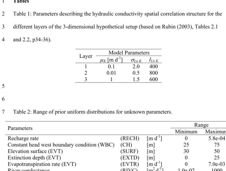
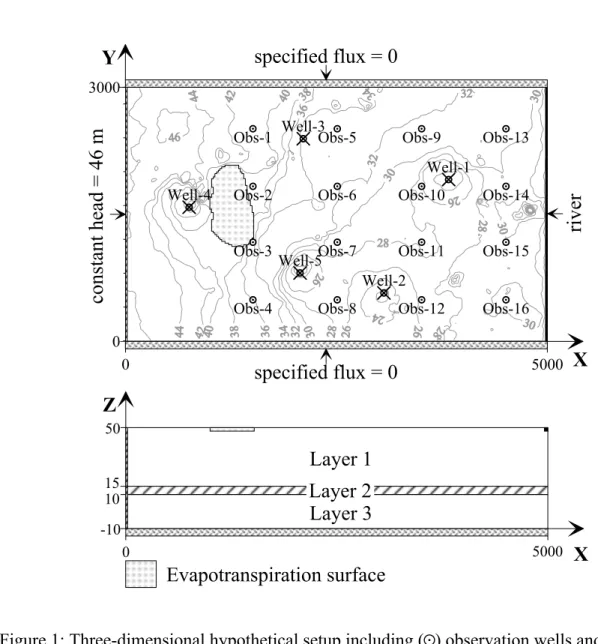
3. Three-dimensional hypothetical setup 13
For illustrative purposes, we employ a 3-dimensional hypothetical setup for which the true 14
conditions are known (Figure 1). Lateral dimensions are 5000 m (E-W) by 3000 m (N-S) 15
discretised in 25 m by 25 m grid cells. The system extents over 60 m in the vertical direction, 16
with undisturbed layer thicknesses of 35 m (upper aquifer), 5 m (middle aquitard) and 20 m 17
(lower aquifer). We assume statistically homogeneous deposits with a constant mean 18
hydraulic conductivity K (see Table 1). Smaller-scale variability is represented using the 19
theory of random space functions, adopting isotropic exponential covariance functions for log 20
K in all layers. The spatial distribution of the hydraulic conductivity in the layers of the
21
example setup, as well as any other realization of the hydraulic conductivity field used in this 22
work, is generated using the sequential Gaussian simulation (sGsim) algorithm of the 23
Geostatistical Software Library (Deutsch and Journel, 1998). Parameters of the covariance 24
function of log K for the different layers are presented in Table 1. 25
Simulation of steady-state flow is performed using Modflow-2000 (Harbaugh et al., 2000). 1
At the north and south boundaries, as well as at the bottom of the lower layer, zero gradient 2
conditions are imposed. A uniform recharge of 1.4 x 10⁻⁴ m d-1 is applied to the top layer. At 3
the west boundary a constant head h = 46 m is defined. The east side of the domain is 4
bounded by a 10 m-wide river with a constant stage of 25 m. The river bottom is at 20 m, 5
defining a constant river water depth of 5 m. It is underlain by 5 m-thick sediments with a 6
vertical hydraulic conductivity of 0.1 m d-1. Five pumping wells are distributed in the area 7
producing a total of 2450 m3 d-1 from the lower aquifer (Figure 1). An evapotranspiration 8
zone, delineated by the polygon in Figure 1, is defined with an evapotranspiration surface 9
elevation at 43 m, an evapotranspiration rate of 1.37 x 10⁻³ m d-1 and an extinction depth of 5 10
m. 11 12
The resulting “true” groundwater head distribution for the top layer is presented as an overlay 13
in Figure 1. The ambient background gradient from west to east is strongly influenced by the 14
drawdown around pumping wells, the evapotranspiration zone as well as by local effects of 15
spatially varying hydraulic conductivity. From the “true” groundwater head distribution for 16
layer 1, values are selected at the 16 locations defined by the observation wells in Figure 1, 17
which are used to estimate the likelihood weights in the evaluation of different simulators. 18
19
4. Implementation of the methodology and numerical analysis 20
4.1. Implementation of the GLUE-BMA approach 21
We consider 7 alternative conceptual models with increasing complexity to describe the 3-22
dimensional hypothetical setup described in section 3, namely: (1), (2) and (3) one-layer 23
models with mean K and spatial correlation law of layer 1 (1Lhtg-L1), layer 2 (1Lhtg-L2) and 24
layer 3 (1Lhtg-L3) of the hypothetical setup, respectively; (4) a one-layer model with average 25
mean K and spatial correlation (1Lhtg-AVG); (5) a two-layer model with mean K and spatial 26
correlation taken from layer 1 and layer 3 (2Lhtg); (6) a two-layer quasi-three dimensional 27
model with mean K and spatial correlation taken from layer 1 and layer 3, and mean K of 1
layer 2 used to define the aquitard (2LQ3Dhtg); and (7) a three-layer model based on the 2
spatial K distributions of layer 1, layer 2 and layer 3 (3Lhtg). All conceptual models comprise 3
a total aquifer thickness of 60 m and are forced by identical types of boundary conditions. 4
5
The dimensionality of the analysis is confined by considering uncertainty only in the input 6
variables and parameters related to the evapotranspiration process, lateral boundary 7
conditions, river description and recharge process, i.e., input variables and parameters that are 8
common to all setups. Values are sampled from uniform prior distributions for the unknown 9
inputs and parameters with ranges defined in Table 2. Unconditional realizations of the 10
hydraulic conductivity field are generated with the same mean K and spatial correlation law 11
as the respective layers in the hypothetical setup (Table 1). For the 1Lhtg-AVG 12
conceptualization the average of these values is used. 13
14
For the simulation, parameter and input vectors sampled using a Latin Hypercube Sampling 15
(LHS) scheme, are combined with unconditional hydraulic conductivity realizations and 16
consequently evaluated under each conceptual model. Based on the evaluation of a set of 17
initial runs, a rejection threshold is defined corresponding to a maximum allowable deviation 18
of 5 m at any of the 16 observation wells depicted in Figure 1. A point rejection threshold 19
rather than a global rejection threshold is chosen because under the latter criteria strong 20
deviations at certain locations (typically in the vicinity of pumping wells) may be offset by 21
small deviations at other wells. For each conceptual model, predictive distributions for the 22
sixteen observation wells depicted in Figure 1 and different components of the groundwater 23
budget (recharge inflows, groundwater inflows/outflows from the west boundary condition 24
(WBC), river gains, and evapotranspiration (EVT) outflows) are obtained from the ensemble 25
of likelihood weighted predictions. Sampling from the prior input and parameter space 26
continued until the first and second moment of these predictive distributions stabilized. 27
4.2. Approach to assess sensitivity to prior model probabilities 1
To analyze the sensitivity to different values of prior model probabilities, the prior model 2
probability space of the 7 alternative conceptualizations is discretised into 25 equidistant 3
intervals of 4% probability each. To avoid extremely low model probabilities that reject with 4
high certainty one of the proposed alternative conceptual models, the lowest probability
5
intervals are discarded from the analysis (this implies that the highest probability of a model 6
is 1-6*0.04 = 0.76). From the remaining 19 probability intervals the lowest value of each 7
interval is retained, resulting in the following set of potential prior model probabilities for 8
each of the 7 alternative conceptual models P = [0.04, 0.08, …, 0.76]. Subsequently, all 9
combinations that fill the prior probability space conditional on Μ , i.e., for which 10
( )
1 M 1 K k k p = =∑
(243 vectors of 7 elements), are formed. This yields a total of 132,861 11potential discrete sets of prior model probabilities that are used to numerically analyze the 12
sensitivity of the posterior model probabilities (weights in equation 1), multi-model 13
predictions and conceptual model uncertainty estimation to prior model probabilities. 14
15
4.3. Constrained maximum entropy approach to assess value of prior knowledge 16
The value of prior knowledge about the plausibility of the 7 alternative conceptual models in 17
assessing conceptual model uncertainty is evaluated following a constrained maximum 18
entropy method (Ye et al., 2005). The method aims to find discrete sets of prior model 19
probabilities that maximizes Shannon’s entropy H (Shannon, 1948) given by 20 21
( )
( )
1 M log M K k k k H p p = = −∑
(7) 22 23 and subject to 240 1,..., 0 1,..., i j h i I g j J = = = = (8) 1 2
where hi and gi represent quantitative relations that reflect prior knowledge about the 3
plausibility of the alternative conceptual models. In equation (7) p
( )
Mk is the prior model 4probability of the k-th conceptual model contained in the ensemble Μ of dimension K. In the 5
case that alternative sets of constraints (reflecting different knowledge states) are proposed 6
and when not enough data are available to assess the quality of model results, Ye et al., 7
(2005) advocate selecting the set that: (i) maximizes entropy H, (ii) presents a minimum 8
entropy among proposed sets and, (iii) maximizes the likelihood for Μ given by the 9
normalizing term in equation 2. 10
11
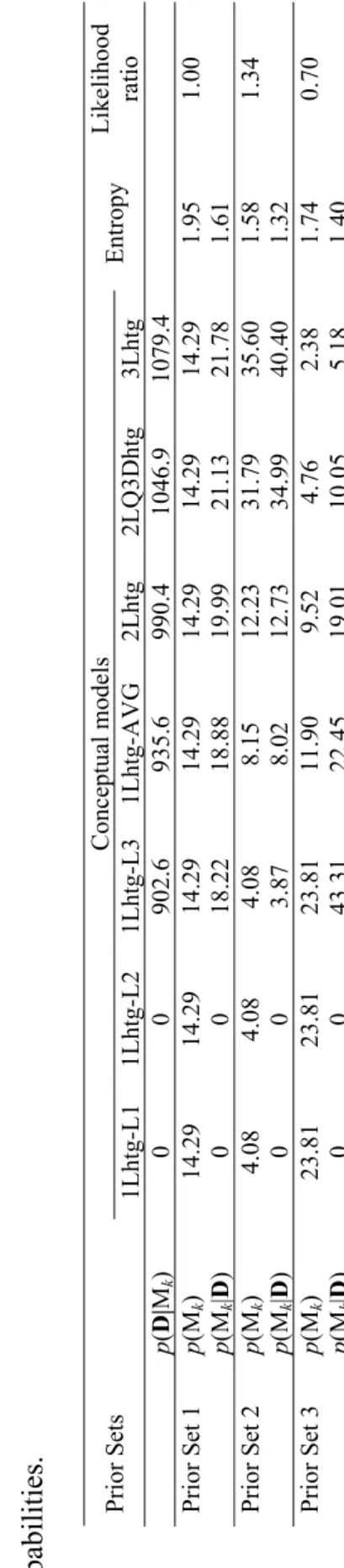
For illustrative purposes we define 3 different prior knowledge states: (i) Prior Set 1, 12
corresponding to a set of uniform prior model probabilities p
( )
Mk =1 K, reflecting a state 13of complete ignorance about the plausibility of the alternative conceptual models; (ii) Prior 14
Set 2, corresponding to a set where alternative conceptual models receive higher prior 15
probability as they approach the 3-dimensional hypothetical setup described in section 3 and, 16
thus, reflecting relevant and proper prior knowledge about the alternative conceptualizations; 17
and (iii) Prior Set 3, corresponding to a set where prior model probabilities are inconsistent 18
with the degree of similarity between the alternative conceptual models and the 3-19
dimensional hypothetical setup and, thus, reflecting improper prior knowledge about the 20
alternative conceptualizations. 21
22
We adopted the following set of constraints to reflect the information contained in the three 23
proposed prior knowledge states 24
Set 1: ( )
( )
( )
( )
( )
( )
( )
( )
( )
( )
( )
M 1 1 1 1 6 1 2 3 4 5 6 7 max M log M M 1 ... : M M M M M M M k K k k p k K k k H p p h p g g p p p p p p p = = = − = − = = = = = =∑
∑
1 2 Set 2: ( )( )
( )
( )
( ) ( )
( ) ( )
( )
( )
( )
( )
( )
( )
( )
( )
M 1 1 1 1 1 2 2 2 3 3 4 3 4 5 4 5 6 5 6 7 6 max M log M M 1 : M M 0 : M M 0 : M 2.0 M 0 : M 1.5 M 0 : M 2.5 M 0 : M 1.1 M 0 k K k k p k K k k H p p h p g p p g p p g p p g p p g p p g p p = = = − = − − = − = − ≥ − ≥ − ≥ − ≥∑
∑
3 4 Set 3: ( )( )
( )
( )
( ) ( )
( ) ( )
( ) ( )
( ) ( )
( ) ( )
( ) ( )
M 1 1 1 1 1 2 2 2 3 3 3 4 4 4 5 5 5 6 6 6 7 max M log M M 1 : M M 0 : M M 0 : 0.5 M M 0 : 0.8 M M 0 : 0.5 M M 0 : 0.5 M M 0 k K k k p k K k k H p p h p g p p g p p g p p g p p g p p g p p = = = − = − − = − = − ≥ − ≥ − ≥ − ≥∑
∑
5 6For Prior Set 1 (uniform prior model distribution) the solution to the optimization problem is 7
known to be H = log K = 1.95 (see, e.g., Applebaum, 1996, p. 100) with p
( )
Mk =1 7. For 8Prior Set 2 and 3 the nonlinear optimization problem is solved numerically using a sequential 9
equality constrained quadratic programming method implemented in an R interface (Tamura, 10
2007) for the code DONLP2 (Spellucci, 1998). The result of these optimization problems are 11
three optimized sets of prior model probabilities for the 7 alternative conceptual models that 1
are in agreement with the quantitative relations (constraints) expressing the prior knowledge 2
states. The optimized values are presented in Table 3. These three sets of prior model 3
probabilities are samples from the full range of possible prior probability combinations, 4
approximated here by the ensemble of discrete sets. It is important to note that the values of 5
the constants in the constraints for Prior Set 2 and 3 were set as an example. Other values for 6
these constants would result in different prior model probabilities, however, still reflecting 7
prior knowledge. Consequently, the present analysis is conditional on the proposed ensemble 8
of alternative conceptual models, Μ , and to the potential quantitative relations among them, 9
i.e., hi and gi. 10
11
5. Results and discussion 12
In the numerical analysis, for the alternative conceptual models 1Lhtg-L1 and 1Lhtg-L2 none 13
of the simulations were accepted, as all of them failed to meet the criterion of a maximum 14
allowable departure of 5 m from the observed heads. This suggests that approximating the 15
“true” 3-dimensional hypothetical setup using only information from layers 1 and 2 (see 16
Table 1) is not supported by the training data D (i.e., observed head at 16 observation wells). 17
Hence, the posterior probability of these conceptual models was set to zero and they were 18
discarded from the posterior analysis. 19
20
5.1. Sensitivity of posterior model probabilities to prior model probabilities 21
The sensitivity of the posterior model probabilities to prior model probabilities for the 5 22
retained conceptual models is presented in Figure 2. In this figure, vertical columns represent 23
posterior model probabilities (estimated using equation 6) corresponding to the 132,861 24
nonzero discrete sets of prior model probabilities described in section 4.2. It can be seen that 25
the posterior model probabilities are sensitive to values of prior model probabilities for all the 26
retained models. It should be noted that the increase of the posterior model probabilities for 27
the 5 retained conceptual models, i.e., nearly all points lie above the bisector curve, is caused 1
by the fact that 2 out of 7 alternative conceptual models were discarded from the posterior 2
analysis based on the information contained in the training data D. As a consequence, the 3
share in the prior probability space of the discarded conceptualizations is redistributed over 4
the 5 retained conceptual models when filling the posterior probability space (i.e., sum of 5
posterior probabilities should equal to 1). This explains why in most cases the posterior 6
probability is larger than the prior probability for the retained models. Notwithstanding, for 7
alternative conceptualizations 1Lhtg-L3 (Figure 2a) and 1Lhtg-AVG (Figure 2b) values of 8
posterior model probabilities below the bisector curve can be found, suggesting that less 9
weight is assigned a posteriori to these models. For alternative conceptual models 2Lhtg 10
(Figure 2c), 2LQ3Dhtg (Figure 2d) and 3Lhtg (Figure 2e), on the other hand, posterior model 11
probabilities are always higher than prior model probabilities, this being more noticeable for 12
model 3Lhtg. 13
14
From Figure 2 it is also seen that the uncertainty in the estimation of posterior model 15
probabilities (expressed by the range of the vertical columns) is maximum when there is no 16
clear preference a priori for a given conceptual model. On the contrary, the range of potential 17
values for posterior model probabilities is reduced when an alternative conceptual model is 18
preferred over the others. 19
20
Results for the three example sets of optimised prior model probabilities are also included in 21
Figure 2 and are summarized in Table 3. Results confirm that posterior model probabilities, 22
p(Mk|D) are largely influenced by the selection of a set of prior model probabilities. For Prior 23
Sets 1 and 2, all retained models received more weight after conditioning. For Prior Set 2, on 24
the other hand, the posterior probability of the two retained one-layer models was smaller 25
than their respective prior probability, whereas the other 3 retained models received more 26
weight after conditioning. However, for all 3 sets, the relative increase of the posterior 27
probability compared to the prior probability is larger for the models approaching the true 1
setup. 2
3
5.2. Sensitivity of the prior entropy, likelihood ratio and posterior entropy to prior 4
model probabilities 5
The sensitivity of the prior entropy, likelihood ratio (with respect to the non-informative case) 6
and posterior entropy (calculated using equation 7 with p(Mk|D) instead of p(Mk)) is 7
presented in Figure 3 for model 3Lhtg. It is seen in this figure that prior and posterior entropy 8
decreased when prior model probabilities of model 3Lhtg increased. Moreover, the likelihood 9
ratio (with respect to the non-informative case) tends to be maximized (Figure 3b) for a 10
maximum probability of model 3Lhtg. Consider, for example, a prior model probability of 11
0.76 for model 3Lhtg and, consequently, 0.04 for the 6 remaining models. Clearly, this set of 12
prior model probabilities is optimum (globally) in the sense that it minimizes posterior 13
entropy and it maximizes the likelihood ratio. 14
15
For the 3 example sets, the smallest maximum prior entropy, the smallest posterior entropy, 16
which can be interpreted as a measure of residual uncertainty after conditioning on the 17
training data D (Ye et al., 2005), and the largest likelihood ratio (1.34 times that of Prior Set 18
1) are obtained for Prior Set 2. On the contrary, the lowest likelihood ratio is observed for 19
Prior Set 3, which suggests that this set is not in agreement with the information contained in 20
the data and that it constitutes an improper expression of prior knowledge about the 21
alternative conceptual models. Hence, for the problem at hand, a reasonable choice for a 22
discrete set of prior model probabilities is to assign increasing probabilities in function of 23
proximity to the 3-dimensional hypothetical setup, i.e., Prior Set 2. 24
25
5.3. Sensitivity of multi-model predictions and conceptual model uncertainty 26
estimations 27
The sensitivity of the leading moments (estimated using equations 3 and 4) for model output 1
river gains and for three alternative conceptual models (1Lhtg-L3, 2Lhtg and 3Lhtg) is 2
presented in Figure 4. This figure shows that the posterior moments (plates a-f) of the 3
predictive distribution for river gains are rather sensitivity to prior model probabilities. It is 4
also seen that uncertainty in the estimation of the leading moments (expressed as the range of 5
the vertical columns) increased when the corresponding prior model probabilities decreased. 6
Additionally, when prior model probabilities for each alternative model increased, the leading 7
moments converged to different values. The latter suggests that when a model is preferred 8
over the others, i.e., relying only on a single conceptual model, predictions and uncertainty 9
estimations tend to be biased. Moreover, estimation of the leading moments tends to be 10
markedly more biased when prior model probabilities of simpler model 1Lhtg-L3 increased. 11
12
Plates g, h and i of Figure 4 show between-model variances for models 1Lhtg-L3, 2Lhtg and 13
3Lhtg, respectively, which are an expression of the conceptual model uncertainty. In general, 14
the contribution of conceptual model uncertainty to the total spread is sensitive to prior model 15
probabilities. Uncertainty in the estimation of between-model variance (expressed as the 16
range of the vertical columns) increased when prior model probabilities decreased. Moreover, 17
for the alternative conceptual models, between-model variances converged to different values 18
when corresponding prior model probabilities increased. It should be noted, however, that for 19
models 2Lhtg and 3Lhtg the converged values of between-model variances (2.1 × 10³ and 2.8 20
× 10 3 [m3 d-1]2, respectively) were rather similar for a maximum prior model probability of 21
0.76. However, the ratio between-model to total variance was somewhat different (7% and 22
18%, for 2Lhtg and 3Lhtg, respectively) due to the difference in the estimation of total 23
variance for these models. 24
25
Figure 5 shows contour plots of the total variance and between-model variance (expressed as 26
a percentage of the total variance) for model outputs west boundary condition (WBC) 27
inflows, river gains and EVT outflows in the prior model probability space of 1Lhtg-L3 1
(simpler model) and 3Lhtg (model closer to the 3-dimensional hypothetical setup) when the 3 2
remaining alternative conceptual models approach a value near the uniform case (0.16). As 3
consequence, only 52% of the prior model probability space is left to be distributed in the 4
plates of Figure 5. More important than the actual values of the contour lines (which are 5
approximations since the true uniform case has a value of 0.143) is the shape of the surface 6
defined in the prior model probability space. 7
8
Plates a, b and c of Figure 5 show that the rate of change of the total variance (a measure of 9
sensitivity) is much larger in the prior space of model 1Lhtg-L3 (x-axis) compared to the 10
prior space of model 3Lhtg (y-axis). Hence, a more important reduction of the total variance 11
would be expected when prior model probabilities of 1Lhtg-L3 decrease. This suggests that, 12
for the problem at hand, to obtain more accurate multi-model predictions, simpler models 13
should receive less prior weight compared to more elaborated models. In addition, it is seen 14
from plates d, e and f that between-model variances does not fall below 5%, 20% and 12% of 15
the total variance and, on the other hand, they can reach values as large as 12%, 30% and 16
18% of the total variance for WBC inflows, river gains and EVT outflows, respectively. 17
Furthermore, the maximum contribution of between-model variances to total variances tends 18
to be located around the middle area of the figures, which is contrasting with the fact that the 19
non-informative case (uniform prior model probabilities) is not located in this area. 20
21
Overall, Figure 5 suggests that when a conceptual model tends to be preferred over the 22
others, between-model variance tends to be minimum. This is in agreement with previous 23
statements about under-dispersive properties of uncertainty estimations based on a single 24
model. On the contrary, between-model variance tends to be maximum when there is no clear 25
preference for a given conceptual model, suggesting that uncertainty estimations based on a 26
suite of alternative models are more spread. This seems logic since including alternative 27
conceptual models provides a more conservative assessment of uncertainty due to including 1
conceptual model uncertainty. 2
3
Figures 4 and 5 also include values for the three optimized sets of prior model probabilities. 4
Although posterior moments converged to different values for different conceptual models in 5
Figure 4, convergence was in agreement with the values obtained using Prior Set 2 when 6
models approached the “true” 3-dimensional hypothetical setup (see, e.g., plates c, f and i). 7
This supports the idea stated before that Prior Set 2 is a suitable choice to assign prior model 8
probabilities. This is also supported by the evidence provided by the data, which gave slightly 9
higher integrated model likelihood values to model 3Lhtg. It is also seen from Figures 4 and 10
5 that the posterior variance, with respect to the non-informative case (Prior Set 1), 11
significantly decreased when proper prior knowledge (Prior Set 2) was included in the 12
analysis. On the contrary, in the case of improper prior knowledge (Prior Set 3) a significant 13
increase of the total variance was observed. More importantly, between-model variances 14
(plates g, h and i of Figure 4) significantly decreased with respect to the non-informative case 15
(Prior Set 1) when proper prior knowledge (Prior Set 2) was included in the analysis, 16
indicating the value of prior knowledge in reducing conceptual model uncertainty. 17
18
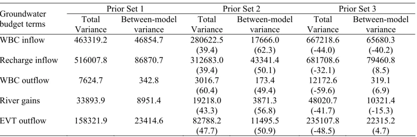
Similar results were found for the other groundwater budget terms (Table 4). With respect to 19
Prior Set 1, total variances decreased between 40 and 60 % when the more informative Prior 20
Set 2 was used. On the contrary, total variances increased between 32 and 60% when 21
improper prior knowledge was included (Prior Set 3). Between-model variances decreased 22
for the informative Prior Set 2 by 50 up to 62% with respect to Prior Set 1. However, the 23
relative contribution of between-model variance to the total variance did not substantially 24
decrease. For example, for EVT outflows obtained using Prior Set 1, the contribution of 25
between-model to total variance is 0.15 whereas for Prior Set 2 this ratio is 0.14. The largest 26
reduction in the contribution of between-model to total variance for Prior Set 2 is observed 27
for river gains; from 0.26 to 0.2. This suggests that the contribution of conceptual model 1
uncertainty to total uncertainty can not be further reduced based only on prior knowledge 2
about the plausibility of alternative conceptualizations. This indicates that other sources of 3
information or conditioning data should be included to further reduce this component of total 4
variance. 5
6
For Prior Set 3 the between-model variances for WBC inflows and river gains increased, 7
whereas for recharge inflows, WBC outflows and EVT outflows, between-model variances 8
decreased compared to Prior Set 1. This erratic behaviour in the between-model variances 9
estimated using Prior Set 3 is explained by Figure 5. 10
11
5.4. Value of prior knowledge about alternative conceptualizations in the goodness of 12
GLUE-BMA predictions 13
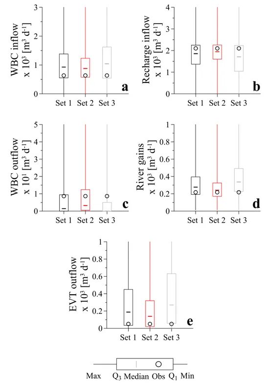
Summary statistics of the posterior predictive distributions for the groundwater budget terms 14
as a function of the optimized sets of prior model probabilities are presented in Figure 6. In 15
this figure maximum values are truncated to enhance visual comparison. Observed values for 16
the groundwater budget terms, obtained from the 3-dimensional hypothetical setup, are 17
captured by the inter-quartile range of Prior Set 1 and Prior Set 2. On the contrary, observed 18
values for WBC outflows, river gains and EVT outflows are not captured by the inter-quartile 19
range of Prior Set 3. Comparing the optimized sets for each plate in Figure 6, Prior Set 2 20
outperforms the other sets since the median values are closer to the observed values and its 21
inter-quartile range is more concentrated, indicating less residual uncertainty after observing 22
data D and incorporating prior knowledge. Hence, this suggests that multi-model predictions 23
obtained using the GLUE-BMA approach in combination with proper prior knowledge (Prior 24
Set 2) outperforms multi-model predictions obtained using sets reflecting a non-informative 25
case (Prior Set 1) and improper prior knowledge (Prior Set 3). 26
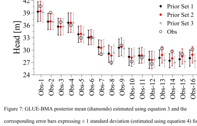
GLUE-BMA predictions for groundwater heads at the locations depicted in Figure 1 are 1
presented in Figure 7. The predictive mean and standard deviation are estimated using 2
equations 3 and 4, respectively. The more pronounced differences in the mean predicted head 3
are observed for observation wells Obs-8, Obs-13, Obs-14, Obs-15 and Obs-16. It is 4
interesting to note that, for these observation wells, observed heads are captured by the 5
interval (± 1 standard deviation) defined around the predicted mean value using Prior Set 2. 6
On the contrary, observed heads are not captured by the interval defined using Prior Set 1 and 7
Prior Set 3. The exception to this is observation well Obs-2, in which none of the optimized 8
sets was able to capture the observed head. It is also shown in Figure 7 that for some 9
observation wells the standard deviations obtained using Prior Set 3 are slightly smaller 10
compared to those obtained with the other optimized sets. However, this gain in accuracy is 11
irrelevant since observed heads are not captured by the intervals defined using Prior Set 3 in 7 12
out of 16 observation wells. Therefore, an over-confident and biased prediction of the 13
observed heads is obtained when improper prior knowledge (Prior Set 3) is used. 14
15
These results confirm that, for the problem at hand, when relevant and proper prior 16
knowledge about the plausibility of alternative conceptual models is included in an analysis 17
following the GLUE-BMA approach, the predictive capacity of the approach is substantially 18 improved. 19 20 6. Conclusions 21
We investigated the influence of prior knowledge and prior model probability definition in a 22
multi-model Bayesian averaging methodology which follows Bayesian formalism and that is 23
used to assess uncertainty in the predictions of groundwater models arising from errors in the 24
model structure, input (forcing) data and parameter estimates. The sensitivity analysis was 25
based on the partitioning of the prior model probability space into discrete equidistant 26
intervals of fixed probability. Subsequently, potential combinatorial sets were permuted to 27
obtain sets of prior model probabilities for 7 alternative conceptualizations. The discrete sets 1
were used to numerically analyze the sensitivity of posterior model probabilities and the 2
leading moments of multi-model predictions of groundwater budget terms. 3
4
Additionally, the value of prior knowledge about alternative conceptual models in reducing 5
conceptual model uncertainty was assessed using three illustrative sets of prior model 6
probabilities. The three sets represented knowledge states expressing a non-informative case, 7
proper prior knowledge, and improper prior knowledge about the plausibility of alternative 8
conceptual models. For each of the sets a nonlinear optimization problem was solved in the 9
form of linear (in)equalities expressing quantitative relationships among the alternative 10
conceptualizations. This resulted in three optimized sets of prior model probabilities in 11
agreement with the prior knowledge at hand. 12
13
For illustrative purposes a 3-dimensional hypothetical setup consisting of 2 aquifers separated 14
by an aquitard, in which the flow field was considerably affected by pumping wells and 15
spatially variable hydraulic conductivity, was used. Seven alternative conceptualizations with 16
increasing complexity were adopted to describe the 3-dimensional hypothetical setup. Two of 17
the simpler one-layer models were discarded from further analysis based on the evidence 18
provided by the data. 19
20
Posterior model probabilities and leading moments of the multi-model predictive 21
distributions showed to be very sensitive to different sets of prior model probabilities. This 22
sensitivity clearly states the relevance of selecting proper prior probabilities in the context of 23
the multi-model approach proposed by Rojas et al., (2008). In addition, increasing the prior 24
model probability of a given alternative conceptual model over the other conceptualizations 25
yielded biased leading moments and under-dispersive uncertainty estimations. 26
We showed that an optimized set of prior model probabilities in agreement with proper prior 1
knowledge outperformed the non-informative and improper prior knowledge cases. 2
Reductions between 40 and 60% (with respect to the non-informative case) for the total 3
variances in model predictions were observed when proper prior knowledge was included in 4
the analysis. On the contrary, total variances increased between 32 and 60% respect to the 5
non-informative case when improper prior knowledge was included. Between-model 6
variances, on the other hand, decreased between 50 and 62% when proper prior knowledge 7
was included. Although in absolute terms, between-model and total variances considerably 8
decreased with respect to the non-informative case when proper prior knowledge was 9
included, for the problem at hand, the ratio between-model variance to total variance, within 10
each optimized set, was not substantially modified. This suggests that the contribution of 11
conceptual model uncertainty to total uncertainty can not be further reduced based only on 12
prior knowledge about the plausibility of alternative conceptual models. This implies that 13
other sources of information or conditioning data should be included to further reduce this 14
component of the total variance. 15
16
The results of this study advocate incorporating proper prior knowledge about alternative 17
conceptual models whenever available. Using a 3-dimensional hypothetical setup and three 18
optimized discrete sets of prior model probabilities, it was shown that the predictive 19
performance of the multi-model methodology proposed by Rojas et al., (2008) could be 20
largely improved when proper knowledge is included. It is expected that combining proper 21
prior knowledge about alternative conceptual models with other qualitative or quantitative 22
sources of conditioning data, such as conductivity data, transient groundwater head 23
information or recharge estimates, will further reduce conceptual model uncertainty. These 24
topics will be subject of future research. 25
Acknowledgments 1
The authors thank the financial support provided to the first author in the framework of the 2
PhD IRO-scholarships of the Katholieke Universiteit Leuven (K.U. Leuven). Assistance 3
provided by Jorge Gonzalez to implement the R scripts is also acknowledged. 4
References 1
Ajami N, Duan Q, Gao X, Sorooshian S. 2005. Multi-model combination techniques for 2
hydrologic forecasting: application to distributed model intercomparison project results. 3
Journal of Hydrometeorology 7(4): 755-768.
4 5
Applebaum D. 1996. Probability and information: an integrated approach. Cambridge 6
University Press: New York; 297. 7
8
Beven K, Binley A. 1992. The future of distributed models – model calibration and 9
uncertainty prediction. Hydrological Processes 6(3): 279-283. 10
11
Beven K, Freer J. 2001. Equifinality, data assimilation, and uncertainty estimation in 12
mechanistic modelling of complex environmental systems using the GLUE methodology. 13
Journal of Hydrology 249(1-4): 11-29.
14 15
Beven K. 2005. A manifesto for the equifinality thesis. Journal of Hydrology 320(1-2): 18-16
36. 17 18
Binley A, Beven K. 2003. Vadose zone flow model uncertainty as conditioned on 19
geophysical data. Ground Water 41(2): 119-127. 20
21
Bredehoeft J. 2003. From models to performance assessment: The conceptualization 22
problem. Ground Water 41(5): 571-577. 23
24
Bredehoeft J. 2005. The conceptualization model problem – surprise. Hydrogeology Journal 25
13(1): 37-46. 26
Carrera J, Alcolea A, Medina A, Hidalgo J, Slooten L. 2005. Inverse problem in 1
hydrogeology. Hydrogeology Journal 13(1): 206-222. 2
3
Deutsch C, Journel A. 1998. GSLIB Geostatistical software library and user’s guide. Oxford 4
University Press: New York; 384. 5
6
Draper D. 1995. Assessment and propagation of model uncertainty. Journal of the Royal 7
Statistical Society Series B (with discussion) 57(1): 45-97.
8 9
Gelman A, Carlin J, Stern H, Rubin D. 2004. Bayesian data analysis. Chapman & Hall/CRC: 10
New York; 668. 11
12
Ghosh J, Mohan D, Tapas S. 2006. An introduction to Bayesian analysis: Theory and 13
methods. Springer texts in Statistics: New York; 352.
14 15
Harbaugh A, Banta E, Hill M, McDonald M. 2000. MODFLOW-2000, U.S. Geological 16
Survey modular water model-user guide to modularization concepts and the
ground-17
water flow process. U.S. Geological Survey. Open File Report, 00-92; 121.
18 19
Harrar W, Sonnenberg T, Henriksen H. 2003. Capture zone, travel time, and solute transport 20
using inverse modelling and different geological models. Hydrogeology Journal 11(5): 536-21
548. 22
23
Hoeting J, Madigan D, Raftery A, Volinsky C. 1999. Bayesian model averaging: A tutorial. 24
Statistical Science 14(4): 382-417.
25 26
Hojberg A, Refsgaard J. 2005. Model uncertainty – parameter uncertainty versus conceptual 1
models. Water Science & Technology 52(6): 177-186. 2
3
Kass R, Wasserman L. 1996. The selection of prior distributions by formal rules. Journal of 4
the American Statistical Association 91(435): 1343-1370.
5 6
Liang F, Truong Y, Wong W. 2001. Automatic Bayesian model averaging for linear 7
regression and application in Bayesian curve fitting. Statistica Sinica 11(4): 1005-1029. 8
9
Meyer P, Ye M, Rockhold S, Neuman S, Cantrell K. 2007. Combined estimation of 10
hydrogeologic conceptual model, parameter and scenario uncertainty with application to
11
uranium transport at the Hanford site 300 area. Report NUREG/CR-6940 PNNL-16396, US
12
Nuclear Regulatory Commission, Washington, USA. 13
14
Neuman S. 2003. Maximum likelihood Bayesian averaging of uncertain model predictions. 15
Stochastic Environmental Research and Risk Assessment 17(5): 291-305.
16 17
Poeter E, Anderson D. 2005. Multimodel ranking and inference in ground water modelling. 18
Ground Water 43(4): 597-605.
19 20
Raftery A, Zheng Y. 2003. Discussion: Performance of Bayesian model averaging. Journal of 21
the American Statistical Association 98(464): 931-938.
22 23
Refsgaard J, van der Sluijs J, Brown J, van de Keur P. 2006. A framework for dealing with 24
uncertainty due to model structure error. Advances in Water Resources 29(11): 1586-1597. 25
Rojas R, Feyen L, Dassargues A. 2008. Conceptual model uncertainty in groundwater 1
modeling: combining generalized likelihood uncertainty estimation and Bayesian model 2
averaging, submitted to Water Resources Research. 3
4
Romanowicz R, Beven K, Tawn J. 1994. Evaluation of prediction uncertainty in non-linear 5
hydrological models using a Bayesian approach. In Statistics for the Environment II; Water 6
Related Issues, Barnett V, Turkman K (eds.). Wiley: New York; 297-317.
7 8
Rubin Y. 2003. Applied stochastic hydrogeology. Oxford University Press: New York; 391. 9
10
Shannon C. 1948. A mathematical theory of communication. Bell System Technical Journal 11
27: 379-423, 623-656. 12
13
Spellucci P. 1998. An SQP method for general nonlinear programs using only equality 14
constrained subproblems. Mathematical Programming 82(3): 413-448. 15
16
Tamura R. 2007. Rdonlp2: An R extension library to use Peter Spellucci’s DONLP2 from R. 17
R package version 0.3-1. http://arumat.ner/Rdonlp2/. 18
19
Wasserman L. 2000. Bayesian model selection and model averaging. Journal of 20
Mathematical Psychology 44: 92-107.
21 22
Ye M, Neuman S, Meyer P. 2004. Maximum likelihood Bayesian averaging of spatial 23
variability models in unsaturated fractured tuff. Water Resources Research 40, W05113, 24
doi:10.1029/2003WR002557. 25
Ye M, Neuman S, Meyer P, Pohlmann K. 2005. Sensitivity analysis and assessment of prior 1
model probabilities in MLBMA with application to unsaturated fractured tuff. Water 2
Resources Research 41, W12429, doi:10.1029/2005WR004260.
3 4
Ye M, Pohlmann K, Chapman J, Shafer D. 2006. On evaluation of recharge model 5
uncertainty: A priori and a posteriori. In Proceedings of the International High –level 6
Radioactive Waste Management Conference, Las Vegas, Nevada; 12.
Figures captions 1
Figure 1: Three-dimensional hypothetical setup including (
R
) observation wells and (P
) 2pumping wells overlain by the groundwater head distribution in the first layer. 3
4
Figure 2: Posterior model probabilities for alternative conceptual models: a) 1Lhtg-L3, b) 5
1Lhtg-AVG, c) 2Lhtg, d) 2LQ3Dhtg and e) 3Lhtg for various sets of discrete prior model 6
probabilities. Symbols represent optimized values of Prior Set 1 ((), Prior Set 2 (#) and 7
Prior Set 3 (+) described in section 4.3. 8
9
Figure 3: Sensitivity analysis in function of prior model probabilities for alternative 10
conceptual model 3Lhtg for: a) prior entropy, b) likelihood ratio (respect to the Prior Set 1) 11
and c) posterior entropy. Symbols represent optimized values of Prior Set 1 ((), Prior Set 2 12
(#) and Prior Set 3 (+) described in section 4.3. 13
14
Figure 4: Leading moments for the posterior predictive distribution of river gains as function 15
of the prior model probabilities of three alternative conceptual models 1Lhtg-L3 (a-d-g), 16
2Lhtg, (b-e-h) and 3Lhtg (c-f-i). Symbols represent optimized values of Prior Set 1 ((), Prior 17
Set 2 (#) and Prior Set 3 (+) described in section 4.3. 18
19
Figure 5: Contours of total variance (a-b-c) and between-model variance (d-e-f) (expressed as 20
a percentage of total variance) for: a) recharge inflows x 104 [m3 d-1]2; b) river gains x 104 21
[m3 d-1]2,and c) EVT outflows x 105 [m3 d-1]2 in the space of prior model probabilities of 22
alternative conceptual models 1Lhtg-L3 and 3Lhtg when remaining models approach the 23
non-informative case. Symbols represent optimized values of Prior Set 1 ((), Prior Set 2 (#) 24
and Prior Set 3 (+) described in section 4.3. 25