3D Visualization Tool for Custom Electronics
Fabrication using Laser Cutter
by
Aradhana Adhikari
Submitted to the Department of Electrical Engineering and Computer
Science
in partial fulfillment of the requirements for the degree of
Master of Engineering in Electrical Engineering and Computer Science
at the
MASSACHUSETTS INSTITUTE OF TECHNOLOGY
May 2020
c
○ Massachusetts Institute of Technology 2020. All rights reserved.
Author . . . .
Department of Electrical Engineering and Computer Science
May 18, 2020
Certified by . . . .
Stefanie Mueller
HCI Engineering Group, MIT CSAIL
Thesis Supervisor
Accepted by . . . .
Katrina LaCurts
Chair, Master of Engineering Thesis Committee
3D Visualization Tool for Custom Electronics Fabrication
using Laser Cutter
by
Aradhana Adhikari
Submitted to the Department of Electrical Engineering and Computer Science on May 18, 2020, in partial fulfillment of the
requirements for the degree of
Master of Engineering in Electrical Engineering and Computer Science
Abstract
In this thesis, we present a 3D visualization tool for a laser cutter fabrication system that can be used to create customized electronic devices. The 3D visualization tool is a two part system. One part generates 3D models of the fabrication output from 2D SVG design files. In addition to the 3D model, the tool also creates an animated visualization of all the fabrication steps involved in creating the design, which includes all the steps for creating the geometry of the design as well as the steps for building the electronic circuit. These 3D models and animations are created using Blender’s Python API, and the results are displayed in a Blender window. This tool has been used to visualize designs with many different features, including LED and quadrotor control circuits, structures with holes, and also 3D structures created through folding.
Thesis Supervisor: Stefanie Mueller
ACKNOWLEDGMENTS
I am very thankful to Professor Stefanie Mueller for allowing me to join her lab as a Meng student, and take part in this project. I would also like to thank her for supporting me in my pursuit of the MEng degree and helping me find TA positions to fund this program. Professor Mueller has also been very encouraging and supporting of the project, and her feedback has always been helpful in making improvements to the project. This thesis covers the 3D visualization tool that is a part of a bigger project, so I would also like to thank my amazing team members who I worked closely with for this project: Martin Nisser, Yuchen Chai, and Christia Liao. Martin helped guide me through the visualization tool every step of the way. He had a lot of ideas on alternatives when I reached roadblocks. Yuchen helped me with the 3D models of the physical hardware that I needed to use in the visualization tool. Christina worked on the Adobe Illustrator design tool so I worked very closely with her to integrate the visualization tool with her tool. There were a lot of panic moments where something broke in the integration pipeline, but thank you for always being so responsive to my messages and debugging inquires. It’s been awesome working together with this team on the project.
I loved being a part of the Human Computer Interaction Engineering Group both as a UROP student and as an Meng student. I would like to thank everyone in the group for being so welcoming. Being a part of this group has been such a wonderful experience for me, so thank you everyone in making it so wonderful. Again, thank you Professor Mueller for this opportunity.
I would also like to thank my sister Upasana Adhikari for helping me create 3D models of some electronic components.
PUBLICATION
The 3D visualization tool covered in this thesis is a part of a larger project that is currently under submission. Some figures used in this thesis are from the larger project that’s currently under submission.
Contents
Introduction 9
1.1 Contribution . . . 11
Related Works 13 3D Visualization Tool 17 3.1 3D Visualization Tool Overview . . . 17
3.2 Design File . . . 19
3.3 Design File Requirement for Visualization . . . 20
3.3.1 Components . . . 20
3.3.2 Anchor . . . 21
3.3.3 Lines . . . 22
3.4 3D Visualization Tool . . . 22
3.4.1 Software Setup . . . 22
3.4.2 Blender User Interface . . . 23
3.4.3 3D Visualization Settings . . . 23
3.4.4 Fabrication Order . . . 24
3D Visualization Tool Implementation 27 4.1 Settings File . . . 27
4.2 Extract Information from Input Design File . . . 27
4.3 Geometry . . . 29 4.3.1 Finding Main Structure Outline, Holes, and Cutaway Pieces . 31
4.3.2 Finding Fold Polygons and Anchor Polygon . . . 35
4.4 Construction of 3D Model in Blender . . . 37
4.4.1 Main Structure . . . 38
4.4.2 Holes . . . 39
4.4.3 Raster Polygons . . . 40
4.4.4 Circuit Elements . . . 41
4.4.5 Folding . . . 42
4.5 Animation of the Fabrication Process in Blender . . . 45
4.5.1 Cutting . . . 46
4.5.2 Folding . . . 48
4.5.3 Rastering Polygons . . . 49
4.5.4 Channel Engraving, Silver Dispensing, and Soldering . . . 50
4.5.5 Pick and Placing . . . 50
4.5.6 Component Functionality . . . 51
4.6 3D Model Scale . . . 52
Evaluation 53
List of Figures
1-1 3D Model for Quadrotor Design . . . 10
3-1 System Overview . . . 17
3-2 Quadrotor Design File and Blender Preview . . . 18
3-3 Creating a Quadrotor Design File . . . 20
3-4 LED Circuit Rastering and Channel Engraving . . . 21
3-5 Quadrotor Blender 3D Model . . . 23
3-6 Blender Settings . . . 25
3-7 Visualization of Fabrication . . . 26
4-1 Fold Lines Group . . . 28
4-2 Electrical Components Groups . . . 29
4-3 Geometric Elements Without Folds . . . 30
4-4 Fold Polygons . . . 31
4-5 Polygons from Cut Graph . . . 34
4-6 Fold Graph Creation . . . 36
4-7 Blender Extruded Polygon . . . 39
4-8 Hole Creation Using Boolean Difference Modifier . . . 39
4-9 Blender Raster Visualization . . . 41
4-10 LED Circuit 3D Model . . . 42
4-11 Determining Fold Section . . . 44
4-12 Animation Speed Widget . . . 46
4-13 Cutting Line Visualization . . . 48
4-14 Cutting Hole Visualization . . . 48
4-16 Channel Engraving, Silver Dispensing, and Soldering Visualization . . 51
4-17 Pick and Place Visualization . . . 51
5-1 Visualization of Different Designs . . . 54
5-2 Folding Angle Approximation . . . 55
Introduction
Fabrication tools such as 3D printers and laser cutters provide means of creating customized objects of wide variety. These fabrication tools can also be altered to provide customization of objects outside of normal use case. For example, the laser cutter is primarily used to make cuts to a sheet of material; thus the output products are typically limited to 2D. However, by defocusing the laser, it is possible to use the laser cutter to bend the material instead of cutting it. When laser is defocused, the laser beam is applied over a larger section of area instead of a single point. The heat applied over the area does not cut the material, but it is enough to allow the material to bend down due to its weight. This method allows users to gain another dimension, enabling users to create 3D structures with the use of a laser cutter [11].
Laser cutters are intended for creating 2D elements, and thus designs drawn to be used with the laser cutter are also drawn in 2D. However, when an additional dimension is introduced to the fabrication, it can be difficult for users to visualize how their fabrication result will look like. In order to visualize the fabrication result, computer aided design (CAD) software can be used to draw the 3D model. Yet, CAD software has a high learning curve and is not something all users are familiar with. Thus, it would help users if there was a visualization tool where they can create their design in 2D (something they are already familiar with), and the software would generate the 3D model from the 2D design.
In this thesis, we introduce a 3D visualization tool to help users visualize their de-signs for a system that uses a laser cutter that has been modified to create customized electronic devices. Users can create their designs in 2D and view the 3D model of the design using this visualization tool. In addition to providing the 3D model, the
visualization tool will also provide a step-by-step visualization of fabrication process for creating the design. Using this visualization tool, users can easily see what the fabrication result looks like. If there are a lot of folds in the structure, users can dou-ble check the order of folding from the visualization tool before actual fabrication. If there are any mistakes in the design, the visualization would help catch it. This can help users save time and resources. Figure 1-1 shows the 3D model generated by our visualization tool for a quadrotor 2D design file.
Figure 1-1: Input to our visualization tool is a 2D design. In (a), we have a design for a quadrotor. (b) shows the 3D model created by our visualization tool for this quadrotor design.
The visualization tool in this thesis is a part of a larger project. The larger project is a system that can build customized electronics of various shapes using a commercially available laser cutter. The geometry of the customized device can be created using the laser to cut (or fold) the acyrlic laser cutter material. The laser cutter is equipped with a mechanical attachment that has a dispenser mechanism for drawing the circuit traces by dispensing silver and a pneumatic mechanism that can be used to pick up and place components such as resistors and batteries. The dispensed silver circuit traces by itself is not conductive, so the laser can be used to make the circuit traces conductive by curing the silver. By defocusing the laser, we can then expand our electronics to 3D structures. The goal of this system is to make the entire fabrication process automated from start to finish. To automate the fabrication process, we can program the laser cutter. Laser cutters can be programmed using a scalable vector graphics (.svg) file. In the .svg file, lines can be color coded to perform
a different function: e.g. red for cutting, black for engraving [2]. Additional colors can be added to introduce more options with laser cutting as well. For example, this feature can be used to add a color that programs the laser cutter to defocus the laser. With automation in mind, the ability to see the visualization of the fabrication process beforehand can be very helpful for users of this system.
1.1
Contribution
The larger project was a collaborative team effort between several members of the lab: Martin Nisser, Yuchen Chai, Christina Liao, and me. I worked on creating the 3D visualization tool, and the focus of this thesis will be on the 3D visualization tool. As the 3D visualization tool is closely tied to the user interface for designing the electronics in the system, I worked closely with Christina to set requirements for the integration of the user designed files to the 3D visualization tool so they are of a format the visualization tool can parse. Christina worked on the Adobe Illustrator user interface referenced in this paper. The pronoun ‘we’ will be used throughout the thesis, as the larger project was a team effort; however, the work on the 3D visualization tool that is covered in detail in this thesis is my own. For the rest of this thesis, ‘system’ will be used to refer to the larger project.
Related Works
Although the 3D visualization tool covered in this thesis is specific to the needs of the system, similar work for visualization can be found in folding of origami, dielines for packaging boxes, and research on fabricating functional devices. As this project is a part of the larger project that aims to provide a novel way of automatically fabricating custom electronics through the use of laser cutter, the work on this thesis is also related to research where modifications are introduced to existing fabrication tools to created customized electronics.
Origami is a great example of taking a flat 2D structure and transforming it into a 3D structure through the use of folds. Algorithms to determine the folding and unfolding of origami has been studied extensively [3]. The folding of origami and the folding problem for this project both have to fold based on a set of provided constraints. The type of 3D shapes that can be created by folding on a laser cutter is generally limited to simple fold structures [7]. Additionally, the defocused laser helps bend the material, but it cannot be done without the weight of the material [11]. Thus, all the folds will always be in one direction: down. The degree of each fold also depends on the exposure time of the defocused laser and the weight of the material. For the dieline folding, 2D drawing is folded following dielines to create a 3D box. Origami [13] is one software that can be used with Adobe Illustrator to display 2D vector graphics as a 3D model; solid lines are cut lines and dashed lines are fold lines. The Origami software requires users to specify certain parameters in the Illustrator file layers, such as which face of the box is “up” and the degree of folding if it is not 90 degrees. Other similar software exists for dieline folding as well, such as Folding Genius 3D [4], however these software are not free for use. These software are also
limited in terms of the 3D visualization needs of our project. It is not possible to introduce thickness to the box. It also does not offer flexibility in introducing additional 3D components to attach to the sides of the box.
In the field of research on fabrication of functional devices, 3D visualization is provided for systems where the user needs to interact with 3D model as part of the design process. In Capricate [15], researchers created a design tool to interactively design conductive traces on a 3D model. To make it easier for users who might not have expertise in creating 3D models, Capricate allows for users to draw 2D geometries on top of an imported 3D model. These 2D geometries reflect what parts the user wants to change in the 3D model to be conductive. The visualization tool then converts the user defined 2D geometry into 3D conductive traces and combines it to the imported 3D model.
PrintPut [1] also provides a way for users to incorporate conductive circuits into the 3D model. PrintPut uses Rhinoceros 3D, a CAD software, as the main interface where users can import a 3D model and indicate locations for desired interactive sensors on the 3D model. This is also another example of where the user designs using 2D geometries, and the visualization does the work of converting the drawing into a 3D model. PrintPut uses post-processing scripts on the user inputs to generate the 3D visualization. As the post-processing pipeline can be algorithmicly intensive, PrintPut also uses a Rhinoceros plug-in called Grasshopper to help generate the resulting 3D model that combines the imported 3D model with the conductive circuit traces corresponding to the desired interactive sensors.
The Capricate and PrintPut works discussed above both cover visualization where the user starts with an imported 3D model, draws 2D drawings to indicate how the model should be modified, and the visualization takes into account both the model and the 2D drawing to generate visualization of the fabrication result. The PipeDream [14] user interface is designed in a similar manner as PrintPut and Capricate. In PipeDream, users can draw 2D curves on a 3D model to indicate how pipes should be incorporated into the model. In this case, the users also needs to start with an existing 3D model.
In FoldTronics [17], researchers explored creating foldable electronics through the use of a honeycomb structure. The work in this paper uses the Rhino 3D software with additional plug-ins. Users design their electronics by first creating a 3D model in Rhino 3D. The FoldTronics plug-in converts the model into honeycomb structures. Upon creation of this structure, users can place electronic components on the hon-eycomb structure. When the design is ready for fabrication, several 2D drawings are generated, representing different layers of the honeycomb structure. These layers can then be printed and manually assembled to create the electronics. In DIY Fabri-cation of High Performance Multi-Layered Flexible PCBs [10], researchers used the laser cutter to create flexible printed circuit boards in a layer by layer approach. After each layer of fabrication work done by the laser cutter, users assembly is required to prepare for the next step in the fabrication process.
The Foldio [12] paper explored electronics that can be customized and printed on a sheet of paper by making modifications to a printer. Once the circuit has been printed, users can then create different designs by making alterations to the paper such as cuts or folds. Users design 3D drawings and this drawing is flatted into a 2D design so it can be printed by a printer. The Foldio visualization takes a 3D input and creates a 2D output. This concept is similar to our visualization tool, however, for our visualization, we want to start with a 2D design and model the 3D to provide a process that is friendly for all users regardless of their 3D modeling experience. The LASEC [6] paper made modification to the material used in fabrication instead of a modification to the fabrication tool itself in order to fabricate stretchable circuits using a laser cutter.
LaserCooking [5] makes use of a laser cutter to prepare food. LaserCooking works by programming different layers into the laser cutter, where the different layers are used for different cooking-related actions. They start with a 3D model and decon-struct the individual 2D layers for fabrication.
Researchers have also explored ways to eliminate the user assembly process when using fabrication tools for creating customized products. Katakura et. al intro-duced robotic manipulator to 3D printer head that enabled automated assembly of
3D printed parts [9]. The LaserOrigami [11] paper avoids the need for user assembly of laser cut parts by relying on bending.
In the works described above, depending on the context of the project, we see the visualization incorporated either directly with the design tool, or as a separate step after the design is created. Regardless of where in the process the visualization is incorporated, there is a common theme: the user interface is designed with usability in mind. Thus, in cases where the user needs to make modifications to a 3D model, users create their designs as 2D drawings, and 3D modifications are created on the 3D model based on the 2D user inputs with the help of the design or visualization tool. However, many of theses visualization tool require users to start with an existing 3D model as a starting point of design. In our work, we keep all aspects of the user design interface to be done in 2D. Additionally, the visualization tool only requires the 2D design. We do not require the user to start with a 3D model. With the visualization tool, we want to support folding features in the larger project. Thus, we do work similar to the work done by software for dieline folding for packaging boxes; however, the constraints of our folding is different from the ones for dielines. Our constraints are set by our system. In addition to displaying the fabrication result for our system, our visualization tool will also support visualization of each step in the fabrication process. Although the works described above do not include such feature, as the overall system’s goal is to fully automate the fabrication of custom electronic devices, being able to see the visualization of the fabrication process is an important part of our visualization tool.
3D Visualization Tool
This section will first give an overview of where the 3D visualization tool fits in the system. Next, the input to the visualization tool (the design file) will be discussed, followed by the requirements on the input file to ensure the visualization tool can create the correct visualization. Finally, the rest of the section will focus on features of the visualization tool and how users of the system can interact with the tool.
3.1
3D Visualization Tool Overview
Figure 3-1: The figure above shows the entire system pipeline, including where the 3D visualization tool fits in the process.
The end-to-end system this thesis is a part of includes both hardware and software components. Figure 3-1 above shows how a user can go through the system to create their own customized devices, from the design to fabrication. In the pipeline, the toolbar plug-in in Adobe Illustrator can be used to create the design. The design file is a SVG file, which is entirely 2D.
The user can choose to launch the 3D visualization tool by clicking the ‘Preview Part’ button on the toolbar. When the ‘Preview Part’ button is clicked, a series of post-processing scripts will run to process the design file into a specified format that the 3D visualization tool can parse. At the end of post-processing, the 3D model is displayed for the design file as it would appear after the fabrication through the use of a laser cutter that is setup with the system configurations. To view the animation of the fabrication process, users can press the space bar.
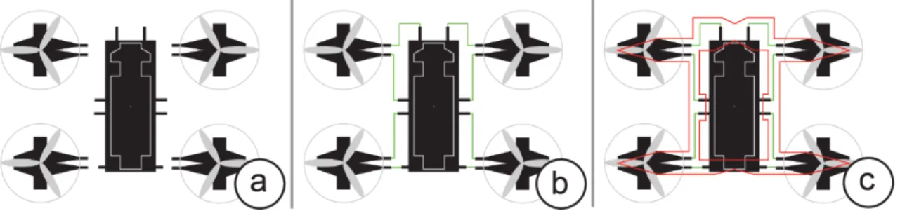
Figure 3-2: This figure shows a 3D model of a quadrotor (c). This model is generated by our visualization tool using the input 2D quadrotor design (b). The visualization is generated by clicking the ‘Preview Part’ button in (a). In the design, the cut lines are indicated by the red lines and the circuit traces are indicated by green lines. The combination of silver and black geometries is used to represent the components. The visualization tool parses all of this information from the design and generates a 3D model that includes the corresponding geometry, components, and circuit traces.
When the user decides a design is ready for fabrication, the user can then generate the laser cutter fabrication file by clicking the ‘Create Laser Cutting File’. Clicking the button triggers a series of post-processing that results in a fabrication file. This fabrication file can be used with a laser cutter equipped with the system hardware to create desired customized device.
3.2
Design File
The design file is what the user directly interacts with in the system. Users start with a blank Illustrator canvas. Users can choose components from the system toolbar and place them where they want. They can draw circuit traces between the components to indicate how the electrical connections should be created, and draw the geometry of their desired customized device by determining what parts should be cut. Users can also choose to add fold lines to their design, which the laser cutter will fold instead of cutting. If there are fold lines present in the design, users will also be asked to indicate what part of the structure should be anchored. This anchored section indicates which part of the structure should always be in the same plane as the one the laser cutter works with.
Colors are very important in the system, as colors are means of programming different setting on the laser cutter. Red lines represents cut lines. The cut lines indicate how the laser cutter material is cut by the laser. Cyan lines represent fold lines. Fold line means a defocused laser will go over the line, creating bends in the structure. Green lines are used for the silver traces that creates the circuit. Black polygons represent the rastering layer of the laser cutter. Silver colors are purely to aid the user in identifying the components. There are more colors introduced in the post-processing step. Orange lines in the post-processed file indicates anchor cut lines. These lines are called ‘anchor’ because they are the line that is cut by the laser at the very end of the fabrication process. Thus they provide an anchor for the structure to remain parallel to the rest of the laser cutter material plane while the rest of the fabrication steps are carried out. Most of these colors can be seen in Figure 3-3, which shows the progression of a design file for a quadrotor, a design where there is no folding involved.
Figure 3-3: The quadrotor design file was created by first placing the components (propellers and printed circuit board) (a), followed by drawing the electrical connec-tions in green (b), and finally drawing the structure of the of design by indicating the cuts in red(c). The black polygons seen in the components will be rastered on the acyrlic if the rastering option is enabled.
3.3
Design File Requirement for Visualization
There are several requirements in place for the input design file to ensure a design can be properly interpreted by the visualization tool. Some of the requirements are handled during the post-processing of the design file, and some requirements are handled during the creation of Illustrator component library.
3.3.1
Components
During the post-processing for the visualization pipeline, component information needs to be encoded into the design file. For each component, the component ID and center location is required. The ID allows the visualization tool to identify the type of component, and the center location indicates the location where the visualiza-tion tool should place this component. If a component does not have ID or locavisualiza-tion data encoded in the .svg file correctly, it will not appear on the visualization.
Additionally, if a component has been rotated in the design, the rotation degree information must also be provided in the post-processed design file for the visualiza-tion tool to load a component with the correct orientavisualiza-tion. The order in which the components should be placed in the visualization is recalculated in the visualization tool to reflect the order in which components are placed in the system’s fabrication process: place components from left to right, and in case of a tie, top to bottom.
Lastly, if components include black rastering polygons, they must be drawn as either rectangles or polygons in Illustrator. Black lines will not be detected for ras-tering by the 3D visualization tool. Raster polygons for a battery, LED, and resistor can be seen in Figure 3-4.
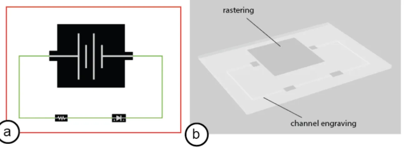
Figure 3-4: In (a) we have a simple LED circuit design. The black polygons in the design indicate rastering. When the rastering option is enabled, these polygons appear in the visualization, as can be seen in (b). If the channel engraving option is enabled, a channel is created for the circuit traces to sit on. The visualization uses the green wire (circuit trace) lines in the design to create these channel engravings. Channel engravings can also be seen in (b).
3.3.2
Anchor
If there are folds in the design, users are required to indicate what section of the structure is the anchor. During the post-processing step, this anchor is used to do the following: 1) Reorder the fold lines in the correct folding order such that outer most fold lines are folded first. This ensures the correct folding in both the fabrication pipeline as well as the visualization pipeline. When a fold is created, the section of the structure that got folded is no longer within reach by the system. Any fabrication step that relies on the use of a laser requires a line-of-sight between the laser head and a fixed distance to the laser cutter material sheet. This requirement is broken for a section when it is folded. Thus by folding outward in, we avoid a situation where we try to create a fold in a location that is no longer within reach for correct folding. 2) The anchor point is used to introduce anchor lines into the design. This anchor
lines will be cut by the laser cutter. However, they are different from normal cut lines because of the order in which they appear in the process. Cut lines happen early in the fabrication process, while the anchor lines (if they exist) are the last step of the fabrication process.
3.3.3
Lines
For the 3D visualization tool, the cut lines, anchor lines, fold lines, and wire (circuit trace) lines are relevant. Each type of line must be grouped together in the design file with their respective ID tag. In the visualization tool, the type of lines are determined by their group ID tag, not their colors.
Anchor lines, fold lines, and wire lines are optional, but the cut lines are required. The visualization tool requires there to be at-least one cut polygon in the design file. If there are no cut lines, there visualization will not work. Visualization is also not supported if there are cut polygons where certain vertices are not connected correctly.
3.4
3D Visualization Tool
The 3D visualization tool is built using Blender’s python API. Blender is an open-source 3D graphics software. With Blender’s python API, we can build the 3D model and animation purely through a python script without human intervention.
3.4.1
Software Setup
Before the 3D visualization tool can be used, users need to set up Blender 2.80 or 2.81. The visualization is written in Python3 and requires the following additional Python packages: shapely and lxml. To use Blender’s Python API, we have to use Python that was installed with Blender. Thus, these Python packages need to be installed in Blender’s Python. Once the software is setup, the visualization tool is ready for use.
3.4.2
Blender User Interface
When users click on ‘Preview Part’ button, the 3D model for the design appears on a Blender window. Users can interact with the 3D model like with any 3D modeling software. Users can zoom; users can rotate to view the model from a different angle as shown in Figure 3-5. The 3D visualization tool is also equipped with the ability to show the animation of the fabrication process itself to see the creation of the 3D model in a step-by-step manner. Hitting the space bar can be used to start/stop the animation of the fabrication process.
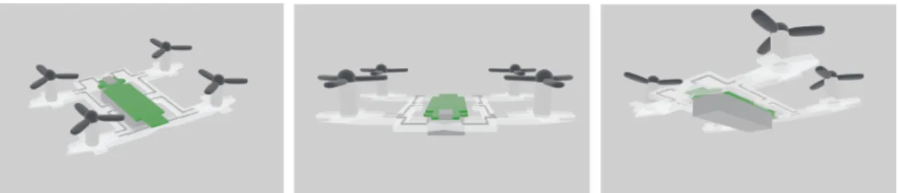
Figure 3-5: We can change the camera angles and zoom from the Blender interface. This can help users see components that might otherwise be hidden from view.
3.4.3
3D Visualization Settings
From the toolbar in Illustrator, clicking the ‘...’ button on the top right brings up a settings menu, where various options for the visualization tool are provided for different parts of the fabrication process.
When the ‘Pick and Place’ is selected, the visualization tool will show the anima-tion of components being placed on the structure one by one, in the correct fabricaanima-tion order. When the ‘Silver Dispensing’ is selected, the visualization tool will show the animation of silver circuit trace being laid out. When the ‘Soldering’ is selected, the visualization tool will show an animation of a laser going through the silver circuit traces to make them conductive. When the ‘Cutting’ is selected, the visualization tool will animate the cutting process of fabrication. This includes both non-anchor cut lines and anchor cut lines. When the ‘Folding’ is selected, the visualization tool will animate the folding process of fabrication. When ‘Component Animation’ is
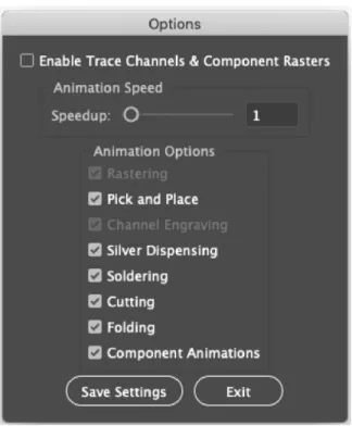
se-lected, components with functions will be animated to highlight their functionality. If there is a propeller, it will spin. If there is an LED, it will light up. Currently, the animation of components functionality is only supported in structures with no folds. To generate a visualization that includes the raster of components or engrave of channels, the ‘Enable Trace Channels & Component Raster’ options must be selected at the very top of the settings menu. When this option is selected, the visualization tool will include rastering and engraving as a part of the fabrication step. If the option is selected, animation options for component rastering and channel engraving will also become available for use under the ‘Animation Options’ section. If ‘Rastering’ is selected, an animation of the rastering will be included in the animation; if the option is not selected, the rastering will still appear in the final 3D visualization, but the step will be skipped in the animation. The ‘Channel Engraving’ option works in the same way as ‘Rastering’, but for the engraving of channels for the circuit traces. Figure 3-6 shows the settings menu where all the different settings for the visualization mentioned in this section can be selected.
3.4.4
Fabrication Order
The system has a set order for the different fabrication process, and the visualization follows this ordering in the animation of the fabrication process: raster the footprint of components (which are the black polygons in the design file) , cut the normal (non-anchor) cut lines, engrave channels for the dispensed silver to sit on, dispense silver to create circuit traces, pick and place components in their correct location, solder the circuit traces to make them conductive, fold the structure based on fold lines, and finally cut based on the anchored cut lines. As can be seen in Figure 3-7, visualization of tools such as laser or a syringe is also used by the visualization tool to help users understand the visualization more clearly.
Figure 3-6: In this configuration, the components rastering and channel engraving options are disabled because the ‘Enable Trace Channels & Component Raster’ option is not selected. With this configuration, the visualization tool will not include the components raster footprint (the black polygons) and the channel engraving as part of the fabrication process.
Figure 3-7: This figure shows different stages of the fabrication for a quadrotor such as the cutting of acyrlic in (a), dispensing of the silver circuit traces in (b), the pick and placement of components in (c), and making the circuit conductive by soldering the silver traces using a laser in (d). This visualization used the settings in Figure 3-6, thus the component rastering and channel engraving options were not included.
3D Visualization Tool
Implementation
This section will cover the implementation details of the 3D visualization tool. This will include the details of how the inputs for the 3D visualization tool are set-up, the parsing of the inputs, the Blender side implementation that relies on the use of Blender’s python API to build the a 3D model from the parsed information, and the animation of the fabrication process.
4.1
Settings File
When the settings are updated in the Illustrator user interface, a settings file is gen-erated and saved in a specified location. This file location is provided when the visualization tool is launched with a click of the ’Preview Part’ button in the Illustra-tor user interface. If the visualization tool does not find the input file at that location, then default settings are used. The default settings correspond to the selection shown in Figure 3-6, where the engrave and raster options are completely disabled, there is no speed-up of the animation, and all the fabrication steps (except engrave and rater which are skipped) will be animated.
4.2
Extract Information from Input Design File
The input design file is a .svg file. This section will cover how information is extracted from the this file.
Each type of line in the input file has an ID associated with it. We use the ID ‘cut’ to refer to non-anchor cut lines, ‘anchor’ to refer to anchor cut lines, ‘wire’ to refer to circuit trace lines, and ‘fold’ to refer to the fold lines. The IDs are encoded in the .svg file through a group tag. Figure 4-1 shows the an example of this grouping being used for fold lines.
Figure 4-1: In this post-processed input .svg file, there are two fold lines. These lines are included in the group with id ‘fold’.
The cut, anchor, and fold lines are used to determine the geometry of the design (Section 4.3). The wire lines are not a part of the geometry. Once we read all wire lines from the .svg file, we subdivide all wires that intersect fold lines into smaller line segments based on the intersection points. This is done to help with Blender-side implementation for folding the structure. Because the rest of the line after a fold line is considered a different line segment, we don’t have to worry about what portion of the line segment gets folded and what portion doesn’t.
There are also many different electrical components, and we use IDs to identify them in the input .svg file. However as there can be multiple components of the same ID, we picked a ID naming convention for electrical component where we check for certain keywords at the beginning of the ID string. We look for the keyword ‘resistor’ for a resistor component, ‘led’ for an LED component, ‘battery’ for a cell battery, ‘nano’ for the Ardiuno nano board, and ‘propeller’ for a propeller component to name a few.
In addition to the ID, center location and rotation information is also encoded inside the group tag. The rotation information is optional, but the location data is required. Each component has their center location encoded using the ‘data-center’ attribute. The ‘data-center’ attribute encodes the x and y coordinates for the com-ponent to indicate its center. From the ‘data-center’ attribute, we can determine the
location of each component, as well as the ordering they should be placed in the pick and place step of the visualization. A component’s degree of rotation is encoded using the ‘data-rotation’ attribute, so this is used in the visualization tool to determine the correct orientation of each component. All the information for electrical components is under a larger group with ID ‘engrave’. Figure 4-2 shows an example how this group of electrical components might look.
Figure 4-2: Inside the group with ID ‘engrave’, we see that there are three electrical components: a battery, a LED, and a resistor. From the ‘data-rotation’ attribute, we see that the led component is rotated 90 degrees. By looking at the ‘data-center’ points, we can determine the location of each component and the order they would appear. Looking at the x coordinates provided with the ‘data-center’ points, there are no two x coordinates that are the exact same, so the the ordering of the components is simply battery, resistor, and led going from smallest x value to largest x value.
The raster polygons are also identified directly from the input file. The raster polygons are all the polygons inside the group with ID ‘engrave.’ Figure 4-2 shows how raster polygons appear in the input file. In the figure, there are seven raster polygons. Only elements with the ‘polygon’ or ‘rect’ tag will be identified by the visualization tool as raster polygons. Line elements will not work.
4.3
Geometry
As the input design file is 2D, to determine the geometric structure of the design, we can’t just read it directly from the file. To determine what the main structure of the design, we need to take the ‘cut’, ‘fold’, and ‘anchor’ line segments in the .svg file and find a way to make sense of it geometrically.
For our case, when determining the main structure, there are four different el-ements to take into account: outline of the main structure, holes, cutaway pieces, and fold polygons. First is the outline of the main structure. In simple designs, this will probably be the only element present. Second are holes in the structure. Holes are polygons consisting entirely of cut lines that fall within the outline of the main structure. Third are holes that do not fall in the structure, which we will refer to as cutaway pieces. Like holes, cutaway pieces are polygons consisting entirely of cut lines. But unlike holes, they are not a part of the structure itself. Cutaway piece in a design is not a common element, however, there might be designs that require them, so there is support added for this feature in the visualization tool. In Figure 4-3, you can see these different geometric components labeled for a design without folds.
Figure 4-3: In this graph representation of the design, red lines indicate cut lines. The connection of these cut lines are indicated by the black circles. The polygon for outline of the main structure is indicated by the thicker lines and circles. There is on hole and one cutaway piece in this structure. In this design, there are no fold lines, thus no fold polygons. Figure 4-5 shows a walk-through of how these polygons are identified by the visualization tool.
The fourth geometric element is something we will refer to as fold polygons. Fold polygons are present if there are folds in the structure. When a structure is folded along a fold line, the new polygon face added to the structure, we are using fold polygon to refer to the polygon that makes up this new face. When folds are present, we also need to identify which polygon is the anchored part of the structure; this polygon will be refered as the anchor polygon. Figure 4-4 shows what the fold poly-gons and anchor polygon is for a structure that contains two folds. Anchor polygon
exists only with the presence of folds. The the following two subsections will cover implementation details for finding these elements.
Figure 4-4: In this graph representation of the design, red lines indicate non-anchor cut lines, orange lines indicate anchor cut lines, and cyan lines represents fold lines. Folding happens from outward in, so the first fold line to be folded is the furthest from the anchor polygon (indicated by the orange lines): Fold Line 1. When the first fold is created over Fold Line 1, the polygon that it creates is the Fold Polygon 1. Similarly, when a fold is created over Fold Line 2, the polygon that is created is Fold Polygon 2.
4.3.1
Finding Main Structure Outline, Holes, and Cutaway
Pieces
Although there are different geometric elements, without context, all of these elements are polygons. Thus to find all the different elements of the design, we need to find polygons in the structure. In order to do this, we construct a graph with all the line segments in the input .svg file. The graph is represented by a dictionary, where each end point of a line segment is a “node” and each node maps to all its neighbors. Once we have a graph, we can find polygons by looking for cycles in the graph, which can be done using shortest path algorithms [8].
First, we look at the graph created only out of cut lines (both anchor cut lines and non-anchor cut lines). This graph will be referred to as the cut graph. When creating this cut graph, we made sure to account for intersection of cut line segments by breaking intersecting line segments into smaller line segments. This is done by creating a new graph and adding all line segments from the cut graph one by one. Before a line segments is added, we first check if it intersects any lines in the new
graph. If it does, the line segment is broken in smaller line segments based on the intersection. These smaller line segments are added to the new graph instead of the original, larger one. Once we have gone through all the line segments, the new graph we created will be our new cut graph.
In the end, we have a cut graph where each edge has equal weight. Breadth-first search is a shortest path algorithm that works when all graphs have equal edge weight. Thus, we can use BFS on the graph to find shortest path from point A to point B. All the points that lie on the shortest path are a part of the polygon including the line segment that has endpoints A and B. Thus to find the a polygon that has the smallest number total of line segments but includes a particular line segment, we can run BFS using the particular line segment’s endpoints as our start and goal. Once we have the cut graph set up where we can use the breadth-first search algorithm, the next step is to find all polygons, all minimal cycle polygons, in this cut graph.
To find all the the minimal cycle polygons of the graph, we use iterations of the BFS. Here are the detailed steps of how this is implemented: 1) Keep a list of all polygon we have found. 2) Create a list of all the line segments in the graph. 3) Check if the found polygons in step 1 combined account for all line segments in the graph. If yes, then end early. Otherwise, check if there are line segments in the list created in step 2. If yes, go to step 4. If no, go to step 8. 4) Remove a line segment from the list randomly. 5) Check if this removed line segment has been used by two or more polygons in the list created in step 1. If the use count is two or more, go to step 3. If the use count is less than two, go to step 6. Each line segment can be shared by at max two polygons. 6) Take the end points from the line segment and run BFS. If the BFS found a shortest path that goes between the two endpoints of the line segment, then we have found a polygon in the graph; go to step 7 to check if this is found polygon is valid. 7) There are two parts in checking if a polygon is valid. First, we need to check that we haven’t found this polygon in a previous iteration (this is possible if you started at a different line segment in the polygon). Second, if this polygon is not a duplicate polygon, we need to check that all the line segments included in this polygon are below the use limit. If there is even one line segment
that is past the use limit, we cannot include this found polygon. If the limit has not been reached on any of the line segments in the polygon, add this polygon to the list from step 1 and increase the use count for all the line segments in the polygon. Go to step 3. 8) Done. The list from step 1 has all the polygons found in the cut graph. Figure 4-5 shows an example showing all the iteration of BFS used to find all the cut polygons.
Once we have all the polygons in the cut graph, the next step is to determine which polygon is the main structure outline. Without the presence of folds, the outline of the main structure is determined by finding the polygon with largest area made out of the cut lines. This relies on the assumption that area of cutaway pieces (if they exist) will also always be smaller than the area of the outline of the main structure. For our use-case, it is okay to make this assumption about the design. If there are folds in the structure, the main structure can be identified through the use of anchor lines. The main structure outline polygon should always consist of the most anchor lines.
Once the main structure has been identified, the rest of the polygons found in the cut graph are either holes or cutaway pieces. To determine whether a polygon is a hole or a cutaway piece, we check whether the center point of the polygon falls within the main structure polygon or not. If it falls within the structure polygon, then it’s a hole. If not, it is a cutaway piece.
Figure 4-5: This shows how iterations of BFS is used to find all polygons from a given cut graph; each row represents an iteration of BFS, where (1) is the first and (5) is the last. Color is applied on top of the cut graph to help visualize each iteration. Red indicates 0 uses, blue indicates 1 use, and light grey indicates 2 uses (the use limit). The black line in the BFS Start-End column is used to indicate the line selected to use as start and goal for the iteration. If a new polygon is found in an iteration, the Found Polygon column indicates the polygon by shading it blue. In each iteration, we can check if we have reached a condition for ending early from the input state. This is the case for (5), where we end early because all lines in the graph are a part of at least one polygon, as indicated by the absences of red lines. (3) does not have a found polygon column because the iteration found the same polygon that was already found in (2).
4.3.2
Finding Fold Polygons and Anchor Polygon
If there are no fold lines present in the design, there are no fold polygons or anchor polygon. If fold lines are present, then fold polygons and anchor polygon exist. To find these polygons, we first add the fold lines to the cut graph from section 4.3.1 are create a fold graph.The created fold graph is not a new graph; it’s a modification to the cut graph that now includes the fold lines.
To create the fold graph, each fold line is added to the cut graph one by one. As each fold line is being added, we first find all intersections of the line with the modified cut graph. For each intersection, we break down intersecting line segment in the modified cut graph line into two smaller line segments and replace the old segment with the two newer line segments. Once all intersections are handled for the fold line, we add the fold line to the graph. When this process is done for all the fold lines, we have the fold graph. For this step, the order of the fold lines does not matter. Figure 4-6 shows a walkthrough of how fold lines are added to the cut graph to create a fold graph.
This implementation to handle the intersection breakdown in fold graph creation was also used in the post-processing step to determine how the anchor cut lines are created as it also needs to look for polygons. There should be no need to include this step again in the visualization since the post-processing should already account for intersections. However, as there is no requirement for the post-processing to do these changes, this code is included in the visualization to ensure that the visualization will not break due to changes made to the implementation of anchor cut line generation. Once the fold graph is created, to find the fold and anchor polygons, we will run iterations of a variation of BFS on the fold graph. It is a variation of the BFS because it will also take into account what nodes and edges should be ignored by the algorithm (treat as not a part of the graph). The BFS will be run once for each fold line; this finds the fold polygons. Then it will run one more time (using the last fold line) to find the polygon for the anchored section. Here are the steps in how the fold polygons and anchored are found from the fold graph. We iterate through the following steps
Figure 4-6: This figure shows how fold lines can be added to the cut graph to create a fold graph. In (a), the red lines represent cut lines, the black circle indicates the connectivity of the line segments that end at the black circle. The cyan line represent the fold line to be added to the graph. The fold line’s end points do not have black circles as the fold lines are not connected with the red lines in the graph yet. (b) shows the cut graph we start with. In (c) we find all intersections of the first fold line with the graph. There are two intersections and they are represented by the blue circles. For each intersection, the red line segment it intersects in the graph is broken down into two smaller line segments. In this example, this step will result in the replacement of two longer line segments in the graph with four smaller line segments. (d) shows the addition of the fold line to the graph. The black circle indicates the fold line is now connected to the graph. If there was only one fold line to add, (d) would be the resulting fold graph.
n + 1 times, where n is the number of fold line present. As the fold lines provided in the input .svg file is in the correct folding order, for the first n iterations to find the fold polygons, we will look for the corresponding nth place fold line. For the last iteration to find the anchor polygon, we will use the nth place fold line as this last fold line must be a part of the anchor polygon.
1) If first n iteration, get corresponding fold line. For the n+1 iteration, use the nth place fold line. 2) Run variation of BFS on the fold graph. Use the endpoints of the current fold line as the start and goal for the algorithm. The nodes that are
ignored is determined in the following way. If the node is an endpoint of a fold line, then it’s allowed to be used twice; otherwise, it’s only allowed to be used in one polygon. As polygons are found, we keep track of whether each node has reached it’s limit. Once it’s reached the limit, it will be ignored by our BFS. As for the edges that should be ignored by BFS, those will be the edges corresponding to all the fold lines that fall after the current fold line in the fold line ordering. This way, the fold lines we have yet to process will not be included when creating a polygon. With these two constraints added to the BFS algorithm, we can find all the fold polygons and anchor polygon.
Once all the polygons are found, we keep track of which fold line actually created each fold polygon. The anchor polygon will not have any fold line with it, as it the last fold line creating the last fold polygon results in the creation of the anchor polygon as a default.
4.4
Construction of 3D Model in Blender
Once the information from the .svg file is parsed, and the geometry has been identi-fied, the Blender Python API is used to construct the visualization. This visualization includes both the 3D model for the design, as well as an animation of how the 3D model is created though a visualization of the fabrication process itself. The visual-ization relies on the use of many different Blender objects to achieve this. Although the animation construction is intertwined with the 3D model construction in the vi-sualisation tool, for clarity purpose,this section will cover how the static 3D model is constructed and section 4.5 will cover how animation is incorporated to the visual-ization.
The channel engraving and silver dispenser model creation is not included in this section because only the result of soldering will be visible in the final 3D model. This will be covered with the animation.
4.4.1
Main Structure
The main structure of the 3D model is built from the polygons found in section 4.3. This structure depends on the existence of folds in the model. If there are no folds, the main structure will only consist of the main structure outline polygon. If there are folds present, the main structure will consist of the fold polygons and anchor polygon.
Whichever case it maybe, the 3D main geometry is created by extruding the polygons. For each polygon that contributes to this geometry, we will create a mesh object. We separate each polygon as a separate mesh object to make folding and other object manipulations required for animation easier to implement. To create a mesh object, we need to provide how the faces of the mesh are constructed by providing a list of vertices (the points) and list of edges or list of faces created by the vertices. Blender supports n-polygon faces (meaning a mesh face does not have to consist of strictly triangles or 4-sided polygons). Thus, we can use the polygons found in section 4.3 directly without modification; we just have to provide list of vertices based on the points in the polygon and the face list will only consist of one face (this represents the polygon) and includes the same points in the same same order as in polygon. With this, we have a mesh with only one n-polygon face, where the face represents the polygon we are trying to create an object out of. This mesh is still 2D. To make it 3D, we will extrude this mesh in the z direction to give it set thickness. This thickness will represent the thickness of the acrylic material we are using in the laser cutter. With the addition of this thickness, the main structure will resemble the acrylic material used in the laser cutter. Figure 4-7 shows how a hexagon 2D polygon can be extruded to create a 3D mesh object. To ensure all the extrude is happening in the same direction, regardless of whether the polygon was created clockwise or counter-clock wise, we take into account the sign of the constructed n-polygon face’s normal. Once we have constructed the 3D mesh objects, we apply a glass-like material to make the visual similar to that of acrylic, which is the material used in the system for fabrication.
Figure 4-7: The hexagon in (a) is converted to a face in a mesh object in (b). This face (b) is then extruded with a set thickness to create a 3D mesh object (c).
4.4.2
Holes
After we have created all the polygon objects that make up main geometry structure, we can introduce the holes in the structure. Each hole is also created as a separate mesh object. The mesh objects are solid, visible objects, but we need the holes to be cutouts in the main structure. Luckily, Blender has support for a Boolean difference modifier, which can be used to subtract one mesh from another. If we have object A and object B, we can create a hole where object B intersects object A by first applying a difference Boolean modifier on object A using object B for the modifier object. The difference is applied on object A so to see the hole left on object A by object B, we hide object B from view. Figure 4-8 shows how this works in Blender.
Figure 4-8: Boolean difference modifier is applied to the grey object in (a) using the green object as the modifier object, resulting in a creation of a hole (b) on the grey object based on the intersection of the green object with the grey object. In (b) the green object is hidden from view so the hole can be seen.
to be created in. However, our main structure could consist of multiple objects. Thus, for each hole, we need to determine which object the hole should be cutout from. We do this step by creating a mapping of holes to the polygons. If there are no folds, we know all holes must be a part of the main outline structure polygon; if it wasn’t a part of the main outline structure; it would have been identified as a cutaway piece, not a hole. If there are folds, we check which polygon it is a part of out of all the fold polygons and anchor polygon. This is done by checking which polygon the center of the hole falls inside, similar to how the distinction between holes and cutaway polygons are made. With this, we have a mapping of holes to polygons. Additionally, when we created the polygons objects for the main structure, we created a mapping from polygons to the corresponding object. Thus, we have all the information to identify which object each hole needs to be applied on, and now we can use Boolean difference modifier to get all the holes on our structure.
4.4.3
Raster Polygons
Raster polygons are polygons that should be engraved into the main structure. They are similar to holes, except that the main structure is not completely cutout based on the raster polygon. Thus, the raster polygons are created very similarly to how hole objects were created. The difference is in thickness of the extrude. For the raster polygon, we pick a thickness that is less than the thickness of the extruded main structure. We also set the raster polygon’s material as a glass-like material, which is the same material as the rest of the main structure . This implementation represents how the real model of an raster polygon looks very closely; however, this method of visualizing the raster polygon is difficult to see. The raster polygon blends with the acrylic material so it’s hard to distinguish the shape of the raster polygon. Thus, we changed our implementation to just show raster polygons as flat polygons that sits on the surface of the main structure. We also changed to material to a non-transparent, solid color that is easier to see in the visualization. You can see a comparison of the old implementation to the new implementation in Figure 4-9.
Figure 4-9: (a) shows a design file of a simple LED circuit with a battery, resistor and LED. With the raster option enabled in the visualization tool, we are able to see the black raster polygons from the design (a) visualized in the model (c). (b) shows a close up of how a raster for the LED component looked in the old implementation; the rectangle is engraved into the structure but it’s hard to see. (d) shows how the same raster polygon appears in the current implementation. It is a 2D rectangle on the surface of the main structure, but it is much easier to see, even in the zoomed out view in (c).
4.4.4
Circuit Elements
The circuit elements such as the electronic components and the wires that connect them are modeled using mesh objects as well.
Due to the complexity of some of the electronic components, we decided it would be best to create a Blender component library for the electronic components. Each electronic component is it’s own Blender file. To use an electronic component in the model, we just need to import the component from the Blender file. To import, we use component ID and the location. We know what file and what object(s) from the file we want to import based on the component ID. We placed the imported object in the location specified as the component’s center location. If there was rotation data associated with the component when it was parsed from the input file, the rotation
will be added to the imported object’s rotation about it’s z axis. Each electronic component can consist of multiple mesh objects, depending on how the component was created in the Blender library.
Unlike the electronic components, the wires are build from scratch in Blender. We used curve objects in Blender to represent wires. Each line segment has it’s own curve object. The curve object is created using the two endpoints of the line segment. The cross-section of the curve object is a circle such that the shape of the resulting curve object is that of a pipe. This closely resembles the circuit traces created by the system. Once created, all curve object are converted to mesh objects. The object that appears in the 3D model is the mesh object. This conversion is done because curve objects don’t have vertices, where as mesh objects have vertices. This matters for some of our animation implementation, where we apply animation to the vertices for each object. We use a silver material for the wire objects. Figure 4-10 shows a visualization for a LED circuit, which includes several electronic components and circuit traces.
Figure 4-10: Here we can see a side by side view of the design (a) and the visu-alization (b) for a LED circuit. In the visuvisu-alization, the battery, resistor, and LED components were imported from the component library and and placed in the location based on the information encoded in the design file. The green lines in (a) represent the wires, which appear as silver traces in visualization.
4.4.5
Folding
In the presence of fold lines in the design, folding is last part in the creations of the 3D model’s main geometry. A fold should occur over each fold line. The order in
which the fold lines are folded are based on the order they appear in the input SVG file. This ensure the same folding order as the one in the system. Each fold line should fold down, as in the system, folds are made possible due to gravity. Thus in the visualization, folding is modeled such that things that are are folded are folded "down" in the negative z axis. In the visualization, the fold angle is always 90 degree, which is an idealization on how folding is done in the system.
As the main structure is one connected piece, each fold line divides this structure into two sections. One section will include the anchor section (from the anchor poly-gon) and the other section will not include the anchor. We will refer to this other section without the anchor as the fold section. For each fold line, we want to fold all elements that fall on the fold section. However, we need to figure out what this fold section is in order to do the folding. The fold section for a fold line is shaded green in Figure 4-11 . However, in order to determine this fold section, we need to determine the connectivity of the structure first.
As there is a mapping from the polygons to objects, we can determine the connec-tivity of the 3D model based on the 2D fold polygons and anchor polygon. For each fold line, we create a mapping to the two polygons that share the fold line. We’ll call these two polygons the share polygons for the fold line. Note that each fold line will always have exactly two share polygons. We’ll also create a mapping for each polygon to all the fold lines it contains. We also already have information about which fold lines create which fold polygon from section 4.3.2.
After all the mapping is created, we use the following means of getting the fold section for each fold line: 1) Create a queue. This will be a queue of polygons. 2) Get the fold polygon for the fold line from the corresponding mapping. Add the fold to the queue. This polygon be the starting place for our connectivity search. 3) Get the share polygons for this fold line. There are two share polygons. One of the share polygons is the fold polygon. We will call the other share polygon the ignore polygon. This is because this polygon is on the same side as the anchor polygon when the structure is divided by the fold line. Thus it will not fold. 4) Create a connected set to track all polygons that make up the fold section. 5) Check if queue is empty. If the
queue is not empty, go to step 6. If the queue is empty, go to step 8. 6) Pop a polygon off the queue. If polygon is not in the connected set, add it to the connected set. Get all the fold lines in this polygon by looking it up in the corresponding mapping. If there are none, go to step 5. Otherwise, go to step 7. 7) For each fold lines found, get the share polygons by looking it up in the corresponding mapping. For each share polygon, if the share polygon is not the same as the ignore polygon, add the share polygon to the end of the queue. Go to step 5. 8) Done. All the polygons that are folded for this fold line will be in the connected set that was created in step 4.
Figure 4-11 shows a visualization of fold section identification for one fold line.
Figure 4-11: In this graph representation of a design, red is for non-anchor cut lines, and orange is for anchor cut lines. In this design, there are two fold lines. The fold line we are currently determining the fold section for is shown by the green line. This fold line divides the structure into two portions. The fold, anchor, and ignore polygons are labeled in (a) as well. Ignore polygon is always on the side that contains the anchor polygon; in this case, the ignore polygon is the anchor polygon. The fold section determined by our algorithm for the current fold line is shaded green in (b).
Once we have determined the connectivity of the structure, here is how the folding is actually implemented in Blender. We go through each fold line in the order they appear in the input. For each fold line, we find the fold section polygons. From the fold section polygons, we can get the corresponding Blender objects for these polygons. The folding is executed by applying a rotation transformation on all of these objects using the fold line as the axis of rotation. The angle of rotation used is 90 degrees. However, in order to rotate such that the rotated portion is folded "down" we might need to change the sign of the rotation to ensure it it rotates downward. We do this by checking whether the fold polygon was created in a clockwise or counter-clockwise direction during the BFS. We determine the direction of polygon creation by calculating the signed area of the polygon. If the polygon was created
counter-clockwise, it will have a positive signed area; if it was created counter-clockwise, it will have a negative signed area. If the signed area is negative (clockwise polygon), we flip the sign on the angle of rotation, making the angle used in the rotation transformation -90 degrees. With this we can ensure correct folding of the structure.
While the structure is being folded, any affected components also need to be folded. Each component can be folded independently of other components. This is because each of these components is a separate Blender mesh object. Additionally, these object will not be shared across two fold polygons. Wire lines could cross over folds; however, as described in section 4.2, wire lines segments that cross fold lines are broken down into smaller line segments when parsed from the input file. Thus, each object can only belong to one object in the main structure. This is similar to the case for holes. Thus, a similar implementation is used to determine which main structure object each component belongs to; we check which polygon the center location of each component falls under and get the corresponding object for that polygon. Since we can determine which polygon these components belong to, we can create a mapping from each of these main structure object to all the components that belongs to the object. Then when an object is a part of the fold section, we can look up all the objects that should also be folded from the mapping. This way, we can account for all components folding as the main structure is folded, even the holes.
4.5
Animation of the Fabrication Process in Blender
This section will cover how the animations for each of the fabrication process is achieved in the visualization tool. This includes animation of cutting, folding, raster-ing, channel engravraster-ing, silver circuit tracraster-ing, solderraster-ing, and pick-and-placing. Addi-tion to these features, the component funcAddi-tionality animaAddi-tion feature is also supported for deigns without folds. For this visualization tool, the animation is created using Blender’s keyframe feature.
The space bar can be used to start/stop the animation. Blender’s default feature was modified such that the animation does not loop upon completion; the animation
is played once and is not played again until triggered again. The animation speed is controlled by changing Blender’s new to old frames ratio for the current scene. Though users can choose the animation speed setting from the Illustrator settings menu before launching the visualization tool, it is also possible to change the ani-mation speed from the Blender user interface itself. When on the Blender window, pressing control+shift+F on a Mac opens a widget where the animation speed can be changed using a slider. This widget with the animation speed slider can be seen in Figure 4-12. We made use of a Blender UI widget Github repository [16] to implement the widget into the Blender user interface.
Figure 4-12: (a) shows a widget that contains a slider to control the animation speed. (b) shows how the widget can appear on the Blender window. This widget can be move to different locations on the window by clicking and dragging. This animation speed widget is launch by pressing control+shift+F on the keyboard.
The keyframe feature allows animations based on changes in various attributes of an object. This is possible by setting a frame for which a certain attribute’s value should be recorded. On the playback of the keyframes, the object will be animated showing how the attribute value changes between the specified frames.
4.5.1
Cutting
For showing the cutting part of the visualization, we need introduce additional objects such as a large piece of acrylic, a laser, a syringe for silver circuit tracing, and another syringe for pick and placement of the components. These objects are not a part of