HAL Id: ineris-03137893
https://hal-ineris.archives-ouvertes.fr/ineris-03137893
Submitted on 4 Jun 2021HAL is a multi-disciplinary open access archive for the deposit and dissemination of sci-entific research documents, whether they are pub-lished or not. The documents may come from teaching and research institutions in France or abroad, or from public or private research centers.
L’archive ouverte pluridisciplinaire HAL, est destinée au dépôt et à la diffusion de documents scientifiques de niveau recherche, publiés ou non, émanant des établissements d’enseignement et de recherche français ou étrangers, des laboratoires publics ou privés.
Underground Rock Dissolution and Geomechanical
Issues
Farid Laouafa, Jianwei Guo, Michel Quintard
To cite this version:
Farid Laouafa, Jianwei Guo, Michel Quintard. Underground Rock Dissolution and Geomechanical Issues. Rock Mechanics and Rock Engineering, Springer Verlag, 2021, �10.1007/s00603-020-02320-y�. �ineris-03137893�
1
Underground rock dissolution and geomechanical issues
Farid Laouafa(1,*), Jianwei Guo(2,*), Michel Quintard(3),
(1)National Institute for Industrial Environment and Risks (INERIS), Verneuil en Halatte, France. (2)School of Mechanics and Engineering, Southwest Jiaotong University, 610031 Chengdu, China (3)Université de Toulouse ; INPT, UPS ; IMFT (Institut de Mécanique des Fluides de Toulouse) ; Allée Camille Soula, F-31400 Toulouse, France and CNRS; IMFT; F-31400 Toulouse, France
(*)corresponding authors ([email protected]),([email protected])
Abstract
Many soluble rocks will dissolve when in contact with fluid such as water. This transformation of rock solid into flowing fluid may trigger the creation of cavities which may further lead to either smooth subsidence or sudden collapse of land surface. Dissolution phenomenon can be of natural or human origin. This paper deals with the problem of the dissolution of underground soluble rocks and the geomechanical consequences such as subsidence, sinkholes and underground collapse. In this paper, rock dissolution and the induced underground cavities are computed using a Diffuse Interface Model (DIM), which does not require to follow interfaces explicitly. We describe briefly the mathematical and physical framework for the dissolution model. We first explain the transition (upscaling) of a multiphysics problem formulated at the microscopic (pore-) scale level to the macroscopic (Darcy-) scale level. Rock material considered in this paper is gypsum, despite that the developed method is also suitable for over soluble rocks (e.g., limestone, Halite). The second part of this paper is devoted to a set of problems dealing with mechanical response of the rock mass in connection with the dissolution process. We discuss the subsidence induced by the dissolution of one or more gypsum lenses, the stability of the covering, and finally the failure of a gypsum pillar in an abandoned quarry. These examples, while they may involve rather theoretical hypotheses, have the virtue of showing the relevance of the method as well as the very diverse issues that it can treat.
Keywords: dissolution, diffuse interface method, gypsum, upscaling, mining, subsidence, stability
1.
Introduction
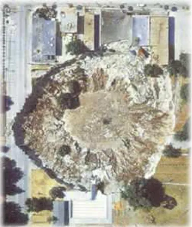
Many problems in geomechanics, such as subsidence, sinkholes and collapses, are related to the dissolution of soluble rocks. So, dissolution of porous rocks is a major concern in geomechanics field since it may cause catastrophic damages. Rock dissolution may create underground voids of large size, leading to a potential risk of instability or collapse of geological formation as illustrated in Figure 1.
2
Figure 1. Land subsidence (sinkhole) in Central Kansas related to underground rock dissolution (after USGS water science).
Dissolution is driven by the flow of an under saturated fluid. For instance, the subsurface water flow or, also, hydraulic conditions through soils and rocks which trigger hydrodynamic? instability onset. The natural or human made hydraulic conditions may evolve with time and change in space. This paper focuses mainly on dissolution of gypsum (CaSO4.2H2O) while the proposed methodologies have a general scope.
Dissolution is also used in industrial activities intensively, for example in the case of salt “solution mining” method. This industrial process extracts underground salt by injecting fresh water through an injection well and produces saturated brine at an extraction well. Such a method is highly suitable in case of thin salt layers located at great depth.
Modeling the multi-scale and multiphysics features of rock dissolution problems requires to address several difficult questions. The first concerns the accuracy needed in the description of solid-liquid interface recession at the macro- (Darcy-) scale level. To achieve this goal, a precise mathematical formalization of physicochemical and transport mechanisms at the micro-scale level is required. The second problem is linked to the description of dissolution at large spatial scales (e.g., in situ scale, site scale). The third is considering the strong physical coupling with other processes, such as rocks mechanical behavior.
The main dissolution rate models are often phenomenological, directly proposed at the macroscopic scale level. The dissolution models which are currently intensively used are based on laboratory tests or in-situ observations. Such models may be considered as describing dissolution in an average sense. Unfortunately, these phenomenological models are unable to take into account accurately multi-scale aspects and issues such as the effect of natural convection or the presence of heterogeneity at the microscopic scale, etc. For instance, a total dissolution rate observed at the laboratory level cannot be extrapolated to the field where hydrodynamic conditions are completely different. Often, interpreting these experiments in terms of intrinsic properties allowing for some up-scaled model and predictions, such as an intrinsic surface reaction rate for instance, is not accessible since it would require a relatively complicated CFD (Computational Fluid Dynamics) analysis. This paper discusses these different questions based on theoretical and numerical analysis of several examples. The starting point of our dissolution problem is the pore scale (micro scale)
3
description of the dissolving surface and the choice of the surface dissolution kinetics. This has been the subject of many studies for various dissolving materials (mainly in chemical or
geochemical scientific domains). Generally, the reaction rate, R , applied as a boundary condition for the micro-scale dissolution boundary value problem for soluble rocks like limestone, calcite, gypsum, or salt follows a general form expressed as (Jeschke et al., 2001; Jeschke and Dreybrodt, 2002):
1 n eq C R k C = − (1) In this expression, k is the reaction rate coefficient, C is the concentration of the dissolved species and Ceq is the thermodynamic equilibrium concentration (also named solubility). The
impact of this boundary condition on transport problem near the surface may be evaluated through the Damköhler number (Da). Damköhler number is a dimensionless numbers used in chemical engineering to relate the chemical reaction time scale (reaction rate) to the transport rate occurring in the system. When Damköhler number is very large, for instance through a very large value of k , this boundary condition tends to the classical equilibrium condition
expressed byC=Ceqat the solid surface. Let us assume that such an approximation is valid and restrict our analysis to two different approaches for modeling the dissolution problem, i.e., the recession of the solid surface. The first one corresponds to a method which follows explicitly the fluid-solid interface. For instance, this can be done using an ALE (Arbitrary Lagrangian-Eulerian) method (Donea et al. 1982). The second approach resolves dissolution using a Diffuse Interface Model (DIM) which transforms the sharp solid-liquid interface into a continuous description (Anderson et al., 1998, Collins et al., 1985, Luo et al., 2012). We will present the physical and mathematical base of the dissolution model and deduce the DIM model using a volume averaging theory. The mathematical problem is formulated at the pore scale and then upscaled to Darcy scale in order to obtain macroscopic balance laws and the associated effective parameters. The workflow is depicted in Figure 2.
Figure. 2. Problem: From micro-scale to large-scale levels
Although the approach proposed in this article is applicable in the context of salt rock (Cristescu and Hunsche (1998), Carter et al. (1993), Bérest et al. (2019), Sadeghiamirshahidi
4
and Vitton (2019)), we will focus on the mechanical consequences of dissolution in a gypsum context.
It must be emphasized, however, that dissolution of rock formations occur in many other contexts. For instance, in Carbon dioxide (CO2) capture and geological storage (CCS), CO2 may dissolve into brines, increasing acidification and dissolution of carbonate species within the reservoir. The reader can refer to the papers of Al-Khdheeawi et al. (2017a-c) and Iglauer et al. (2015) for more details. Similarly, acid injection is currently used to recover the permeability of rock formation surrounding petroleum wells, an engineering technique based on the existence of unstable dissolution fronts (Golfier, F., Zarcone, C., Bazin, B., Lenormand, R., Lasseux, D., Quintard, M., 2002. On the ability of a Darcy-scale model to capture wormhole formation during the dissolution of a porous medium. Journal of Fluid Mechanics 457, 213–254.). These interesting topics and the associated mechanisms are out of the scope of this paper.
In some abandoned mines, gypsum pillars are naturally subjected to many external loads (mechanical, thermal, hydric, etc.) and weathering (e.g., action of water, bacteria), which may degrade their mechanical properties (Castellanza et al. (2008)). A dangerous phenomenon in case of abandoned gypsum and anhydrite mines is water flooding. In the case of time-continuous flooding, the underground water will progressively dissolve pillar rock until failure. To access the short- or long-term stability of the mine, the time evolution of the dissolution process and the recession rate of the water-gypsum interface must be investigated. These natural processes are of direct relevance to gypsum mining. Because gypsum dissolves readily in flowing water, any gypsum mine which becomes flooded on abandonment should be subject to a hydrological survey as advised by Cooper (Cooper, 1988).
Whatever the hydro-geological configuration, the dissolution of gypsum (lenses, pillars, etc.) in the ground raises the questions in terms of geomechanical consequences: subsidence, sinkholes, pillar or cavities stability, etc. (Gysel (2002), Walthan et al., (1981), Toulemont, (1987,1981), Cooper (1988), Bell et al. (2002)). The purpose of the last section of this article is to show theoretically on several 2D and 3D examples, the robustness and the potentialities of the proposed numerical dissolution approach.
The problems to be dealt with from a mechanical point of view will be either elastic or elastoplastic. We will illustrate these questions in the case of subsidence induced by the dissolution of one or several gypsum lenses. In these examples, gypsum lenses are located between porous rock layers. We analyze the evolution of the stability of the recovery as a
5
function of spatial evolution of the dissolution front (water-gypsum interface). We finally analyze the evolution of the stability of an isolated gypsum pillar. All these models have a predictive feature, as they provide the evolution of the deformation mechanisms as a function of time.
2.
Dissolution models
This section first describes a generic pore-scale dissolution model corresponding to dissolution of a soluble solid species considered as a single component (either a true one component system or a mixture that behaves as a single component, in this case referred to as a pseudo-component). The approach can be extended easily to a material having several components (multi-components). In this latter multi-component case, conservation equations (mass, momentum, etc.) should be applied to each component of the physical system. In this paper, only a general idea is given about the upscaling of the pore-scale equations into a macro-scale diffuse interface model. The resulting Darcy scale model can be used to model the dissolution of large cavities or porous formations. The methodology is available for salt, gypsum and even carbonate rocks, provided that local conditions are compatible with the assumption of a pseudo-component. Otherwise, the same methodology must be extended to a multicomponent treatment, which is beyond the scope of this paper.
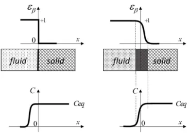
As introduced earlier, we may consider various classes of dissolution models. The first one corresponds to the original dissolution problem involving a sharp liquid/solid interface (Figure 3). In this case, the solid-liquid interface is defined mathematically by a surface at which the liquid concentration is equal to the equilibrium concentration, given our assumption of large Da. To describe the dissolution state, we may introduce a scalar “phase” indicator defined in the whole domain (rocks and fluid). For example, if this scalar is the porosity εβ, it has a value of 1 in the liquid phase and zero elsewhere (or a non-zero value if the “solid” is a true permeable porous medium), with a jump at the solid-liquid interface (left column of Figure 3). Solving the mathematical problem requires special front tracking, front marching numerical techniques, which are often computationally time consuming. This method can face numerical difficulties, in the presence of geometrical singularities (near non-soluble layers). Such difficulties can be circumvented if we do not require an explicit treatment of the moving interface. Instead, partial differential equations are written for continuous variables, such as
β
ε and the mass fraction ωAβ (mass fraction of species A in the β-phase), which leads to a
6
Figure 3. Original dissolution model (sharp interface on the left) and diffuse interface model (on the right).
The original solid/liquid dissolution problem can be described by classical convective-diffusive mass balance and Navier-Stokes (momentum) equations, etc. To develop the DIM model, we start from these original solid/liquid equations to generate averaged or Darcy-scale equations involving effective coefficients (Luo, et al. 2012, Guo et al. 2015) and considering the density as a function of concentration. In the first subsection, the original pore-scale model for the dissolution problem is introduced. In the second subsection, we briefly introduce the upscaling of the pore-scale model into the Darcy-scale equations which are used as the basis for the DIM formulation.
2.1. The original multiphase model
Following our assumption of a pseudo-component behavior, let us consider a binary liquid phase β containing chemical species A and B, and a solid phase σ containing only
chemical species A, as illustrated in Figure 4 (right).
Figure 4: Large-scale (left) and near interface scale (right)
The total mass balance equation for the β-phase, the mass balance for species A in the
β-phase, and the general mass balance equation for σ-phase can be expressed by Eqs. 2(a)-(c), respectively.
(
)
(
)
(
)
(
)
(
)
( ) 0 ( ) ( ) 0 A A DA A t a t b c t β β β β β β β β β β β σ σ σ ρ ω ρ ω ρ ωρ
ρ
ρ
ρ
∂ + ∇ ⋅ = ∇ ⋅ ∇ ∂ ∂ + ∇⋅ = ∂ ∂ + ∇⋅ = ∂ v v vErreur ! Signet non défini.(2)
Here, and denote the density of the β- and σ-phase, respectively. and denote bulk
velocity of the β- and σ-phase, respectively. In the following analysis, the σ-phase is supposed
7
diffusion coefficient. For the pure fluid flow, we will use the Navier-Stokes equations for the momentum balance, i.e.,
2 g p t β β β β β β β β ρ ∂ + ⋅∇ = −∇ +ρ +ζ ∇ ∂ v v v v (3)
wherev , β ∇pβ represents the pressure gradient in the β-phase, ζβ the dynamic viscosity (supposed constant) of the β-phase and g the gravity vector. At the β-σ interface Aβσ , the
chemical potentials for each species should be equal for the different phases. In this case and for the special binary case under investigation, we have the following equality at a given pressure p and temperature T:
(
, ,)
(
, ,)
atAβ Aβ p T Aσ Aσ p T Aβσ
µ ω =µ ω (4) where, ωAσ is equal to 1. It must be emphasized that in the complete binary case, i.e., when
Aσ
ω is not equal to 1, there is also a relation similar to the above equation for the other components. The binary case results in the classical equilibrium condition, i.e.,
at
Aβ eq Aβσ
ω =ω
(5)
where, ωeq is the thermodynamic equilibrium concentration for species A. Note that this
equation is also fulfilled in the reactive case when Da >>1.
The boundary conditions for the pseudo-component mass balance at the solid-liquid interface (of outward normal nβσ) can be written as:
(
)
(
A βDA A)
(
β)
at Aβσ ⋅
ρ ω
β β vβ −wβσ −ρ
β∇ω
β =nβσ ⋅ −ρ
σw σ βσn (6)
where, wβσ is the interface velocity. This equation can be used to calculate the interface
velocity. We can remark that in general we have the following inequality: wβσ ≪ vβ
For gypsum, for instance, the maximum value of nβσ ⋅wβσ is about 9.7 10 m / s,× −8 which is negligible compared to seepage velocities in hydrogeology, which is on the order of 10-5 to 10-6 m/s. A boundary condition corresponding to no jump in the tangential velocity has to be enforced at Aβσ .
The recession velocity wβσ can be expressed as :
1 (1 A )DA A β β σ βσ βσ βσ β β ω ω ρ ρ ⋅ = ⋅∇ − n w n (7)
8
This last equation relates explicitly the recession velocity to the transport flux and can be used to compute the interface movement in ALE method. The dissolution problem is completed with the set of equations to describe the boundary and initial conditions of the fluid domain. Because of the complex movement of the interface, frequent re-gridding is required and the resolution near the interface cannot be very fine, or else it creates rapid unacceptable distortion of the mesh.
Some of the numerical difficulties associated with very sharp fronts can be circumvented by using a Diffuse Interface Method (DIM). Contrary to “interface tracking methods", a diffuse interface method considers the interface as a smooth transition layer where the quantities vary continuously. The whole domain constituted by the two phases is considered to be a continuous medium without any singularities nor a strict distinction of solid or liquid (see Figure 3).
2.2. Darcy-scale non-equilibrium model
A DIM model can be written in an ad’hoc manner or developed more accurately following a porous-medium type of approach. In this subsection, we briefly describe the macroscopic Darcy-scale equations obtained by upscaling the above set of pore scale equations, using the volume averaging theory (Quintard and Whitaker, 1994, Whitaker, 1999). The reader will find in paper (Guo et al., 2016) the details of this change of scale. The representative elementary volumes are schematically illustration in Figure 5. We define the intrinsic average of the mass fraction as
( )
1 1 A A A A V dV V β β β β β β β β ω ε ω− ω Ω = = =
r (8)and the superficial average of the velocity as
( )
1 V dV V β β β = β =εβ β =
β V v v v r (9)where, V is the filtration velocity and Uβ β = vβ β is the β-phase intrinsic average velocity.
Figure 5. Averaging volume at pore scale level and material point position vector (left) and 3-phases model (the third phase may be insoluble species for instance) (right
9
(
)
( ) ( ) ( ) ( ) 1 -A A A A A A A D dA t V βσ β β β β β β β β βσ β β β ρ ω ρ ω ρ ω ρ ω ∂ + ∇ ⋅ = ∇ ⋅ ∇ ⋅ − ∂
c b a d v n v w (10)The different terms express: (a) accumulation, (b)convection, (c) diffusion, and (d) the phase
exchange terms, respectively. Based on several assumptions and some mathematical
treatments of the different equations, we obtain the following control equations for the diffuse interface model (DIM) (Luo et al. 2012)
(
)
(
)(
)
* A * * * . * 1 A A A A eq A t β β β β β β β β β β β β β ε ρ ∂Ω +ρ ⋅∇Ω = ∇ ⋅ ε ρ ∇Ω + ρ α − Ω ω − Ω ∂ V D (11)(
)
(
)
* * * eq A t β β β β β βε ρ
ρ
ρ α ω
∂ + ∇⋅ = − Ω ∂ V (12) and(
)
* eq A t t β σ σ σ β βε
ε
ρ
∂ρ
∂ρ α ω
− = = −Ω ∂ ∂ (13)where, ρβ* is such that ρ ωβ Aβ =ε ρβ β*ΩAβ and
α
is the exchange term between the two phases, which is a non-linear function of εβ.D*Aβ is the macroscopic diffusion/dispersion coefficient, which can be expressed as(
)
* I T I A L T D β β β β β β β β α α α τ ε ε = + V + − V V D V (14)where the tortuosity τβ, the longitudinalαL and transversalαT dispersivities (αL and αT) depend on the pore-scale geometry and possibly εβ. The macroscopic effective coefficients are obtained by solving “closure problems” provided by the theory over different types of unit cells representative of the porous medium, as illustrated in Figure 6.
Figure 6. Examples of various f 1D, 2D and 3D unit cells (after Courtelieris and Delgado (2012)
Closure problems correspond to an approximate solution of the coupled problem: averaged variables/deviations. The approximate solution takes often the form of a mapping such as
(
)
Aβ β Aβ sβ eq Aβ
10
where, ωɶAβ is the concentration deviation and b and sβ β are two closure variables. Solving two sets of boundary value closure problems for b and sβ β allows us to express the macroscopic effective values according to the characteristics at the pore scale.
In other words, the physical properties at the macroscopic level are not "phenomenological" values but built on the basis of physical properties observed-defined at
the microscopic scale. In our case, we obtain the effective macroscopic diffusion tensor DA*β,
the macroscopic effective exchange coefficient
α
and the effective density ρβ* such as:(
)
11 1 A A A D dA b V βσ β β εβ− βσ β εβ− β β = + −
ɶ * D I n b v (16)(
) (
)
1 1 eq A A D s dA V βσ β β βσ β ρ α ω = ⋅∇ −
n (17) * 1 A A β β β β βρ
ρ ω
ε
= Ω (18) We observed that when the saturation at a material point is reached then:0 eq A Cte t β β β
ε
ω
= Ω ∂ = ⇔ε
= ∂ (19) In the case of DIM use for a large-scale cavity dissolution problem involving an impervious rock formation, i.e., not necessarily a real porous medium problem application, the choice of the exchange coefficientα
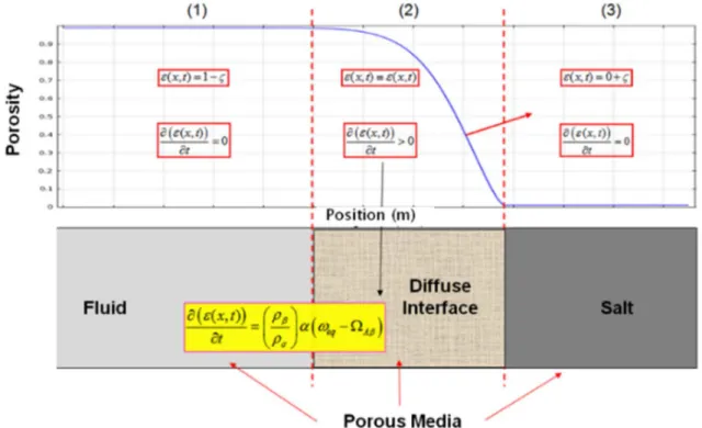
expression as a function of porosity is more arbitrary. It must, however, be observed a null condition when the material point is considered strictly in the fluid phase or strictly in the solid phase. This is illustrated in Figure 7.Figure 7. Porous domains: "fluid"-interface-solid and expression of volume fraction ε
We must underline that, in the DIM model, there is no “pure liquid phase” (Figure 7) since εβ is used continuously to represent the fluid as well as the solid regions. Therefore, the Navier-Stokes equations are not suitable in the rock domain region. We must add a Darcy term in the momentum equation. For instance, we can adopt a Darcy-Brinkman model (Brinkman, 1947) such as
11
( )
(
*)
( )
1 0 A A P β β β β β β β β β µ ρ µ ε − Ω ∆V − ∇ − g − Ω K ⋅V = (21)where the permeability tensor K is a function of εβ . The Darcy-Brinkman equation will approach to Stokes equation when K is very large and will simplifies to Darcy’s law when K is very small. If inertia terms are not negligible, a similar Darcy penalization of Navier-Stokes equations may be used. The resulting DIM equations may be solved with various numerical techniques but in this paper, we will use a COMSOL Multiphysics® implementation. Results are presented and discussed in the next section.
To summarize, the most important assumptions behind the model used in the examples are: 1. the possibility of using a pseudo-component,
2. Damkhöler and Péclet numbers so dissolution is close to the thermodynamic equilibrium boundary condition case,
3. Darcy-scale heterogeneities at a scale smaller than the typical formation scale are not included.
Cases with more complex chemistry may be handled as now indicated in the paper by moving to a multicomponent system. In this paper, we have essentially proposed examples with thin dissolution fronts. In this case, the actual « pore-scale » dissolution has not a great impact (i.e., boundary condition at the solid surface being of reactive form or thermodynamic equilibrium form). This would change the dynamics at the pore-scale but not at a larger scale (a Darcy-scale dissolution front, even very sharp, involves several pore length-scales). This is why we restricted our examples to such cases. Still, in order to compare to an actual site situation, a good characterization of the site is necessary mainly because heterogeneities will impact on the recession velocity.
3.
Dissolution modelling and geomechanical issues
The main goal of this section is to show the potential application of the method outlined in the previous section in terms of mechanical consequences induced by rock dissolution, i.e., the coupling of dissolution processes with geomechanical boundary value problems. The "theoretical" configurations considered below are sufficiently representative of real cases. The cases of flooded rooms in gypsum quarries, void created by dissolution and sinkholes as
12
illustrated in Figures. 8 and 9 are common. In fact, many ground surface failures occur over gypsum beneath Paris (France) (Toulemont, 1987), and investigation of a cavity found in 1975 beneath railway engineering works revealed a failure migrating upwards through the cover rocks from dissolution cavities in a number of gypsum horizons. As advised by Cooper (1988), gypsum mine, which becomes flooded on abandonment, should be subject to a hydrologic survey. Whatever the hydro-geological configuration, the dissolution of gypsum in the ground raises the question of consequences in terms of geomechanical behavior: surface subsidence, sinkholes, caverns or pillar stability, etc. In the 2D or 3D numerical examples under consideration, the dissolution process will generate growing cavities (case of gypsum lenses) or decreasing cross-section of pillars (case of rooms and pillar quarries). Numerous caprock sinkholes at Ripon, U.K. are reactivated by continuous dissolution of gypsum (Cooper, 1988). The mechanical consequences of dissolution can be either a gentle deformation of soil surface or recovery failure and collapse leading to sinkholes (Figure 9).
Figure 8. Views of a pillar in the Rocquevaire abandoned quarry (Bouches-du-Rhône, France) with two different water flooding levels (at two different times 1996 and 2010, by courtesy of Watelet JM, INERIS) and (right) schematic section through a hidden void found within cover rocks of gypsum in Paris (France) railway station underground (After Toulemont (1987)).
Figure 9. Examples of dissolution consequences: (Left) several sinkholes in wood Buffalo National Park (Canada). An interstratal dissolution of gypsum induce a collapse that propagates through dolomite cover beds and (right) (after Walthan et al. (1981), Van Everdingen (1981))
The non-linear coupled time dependent multiphysics problems are solved within the framework of porous medium theory. The mechanical consequences of the dissolution are approached in our geomechanics framework through a simplified analysis. For the mechanical response of the rock mass, we consider only the effect of domain change induced by the dissolution. The dissolution process will generate growing cavities (case of lenses) or decreasing cross-section of pillars (case of rooms and pillars quarries). The domain is supposed saturated and drained. The problems are supposed also isothermal. In fact, there is no particular difficulty to introduce temperature either in dissolution formalism or mechanical problems.
13
In the following 2D and 3D examples, we consider several coupled problems. The first one corresponds to the dissolution of one or more gypsum lenses contained in a porous horizon, which can be located between two layers of marl for instance. And the flow is induced by a natural hydraulic gradient. The second case corresponds to dissolution under an elastic and elastoplastic recovery. Finally, the third scenario is about the dissolution of an elastoplastic gypsum pillar. We will analyze the time evolution of subsidence, surface slope, mass deformation, stability and collapse condition for the roof and for the pillar. These simple examples show the predictive nature of the proposed approach.
3.1 The case of one gypsum lens with elastic or elastoplastic recovery
The first theoretical problem considered is the isothermal dissolution of a cylindrical gypsum lens of 2.5 m thick with a diameter of 5 m (Figure 10). The lens is located in a porous medium located between two permeable domains. Pure water flow is imposed at the inlet at the velocity V of 10-6 m/s, with zero concentration of the dissolved species. All the boundaries of the layer containing the lens are at zero flux, with the exception of the inlet and the outlet boundaries. The permeability K of the gypsum is 10-15 m2 and that of the surrounding medium is 10-12 m2. The dynamical viscosity of water is 10-3 Pa s. All boundaries of the layer are symmetric from a mechanical point of view. The elastoplastic (Mohr-Coulomb) soil/overburden has a Young's modulus of 25 MPa, a Poisson coefficient of 0.3, a cohesion of 0.1 MPa and a friction angle of 30°. The Young’s modulus of the supposed elastic gypsum lens is equal to 35000 MPa.
Figure 10. Mesh and location of soluble gypsum lens and water level.
The density of all materials is taken to be 2000 kg/m3. The model has a vertical plane of symmetry passing through the middle of the lens (Figure 10). Therefore, we will model only half of the domain. On all sides of the model the normal component of displacement is zero (roller plane). The only load is gravity.
3.1.1 One gypsum lens with elastoplastic recovery
In Figures. 11 and 12, we present the 3D shapes of the gypsum lens at different times and the temporal evolution of a cross section passing through the middle of the cylindrical lens,
14
respectively. We observe a significant reduction of the cross-section induced by dissolution, with the initial cylindrical shape preserved.
Figure 11. Gypsum lens (red) at different times (0, 10, 40 and 60 years).
Figure 12. Time evolution of a cross section passing through the middle of the cylindrical lens, with the contours corresponding to time of 0, 20, 30, 40, 50, 60 and 65 years, respectively.
The size of the cavity increasing with dissolution will induces plasticity or failures in the overburden. If the cavity has a significant size and/or weak mechanical properties, the effects of dissolution can result in subsidence or a sinkhole creation. In Figure 13 we show the spatial
distribution of the effective plastic strain expressed by
ε
ep: 2(
)
3
ep p p
ij ij
d d
ε
=
ε
ε
for three time instants (20, 40 and 60 years), where we observe the extension and the distribution as a function of the intensity of the lens dissolution.Figure 13. Effective plastic strain distribution in the recovery after 20, 40, and 60 years (top) and isovalues of the effective plastic strain distribution in the recovery after 20, 40, and 60 years.
In Figure 14 we show the time evolution of the volume integration of the effective plastic
strain _ ep
Overburden
Int EP=
ε
dv.The purpose of this integration is not so much to determine a particular value from a physical point of view but to show the temporal evolution of the plasticity in the recovery. We see that it increases continuously with time, thus vary with dissolution and remains constant when the gypsum lens is completely dissolved. Figure 15 shows the evolution of the vertical displacement w, for point A on the bottom of recovery and point B at the surface, with both two points in the middle of the model. One may observe the vertical displacement as dissolution proceeds.
15
Figure 14. Time evolution of the volume integration of the effective plastic strain over the overburden.
Figure 15. 3D distribution of vertical displacement when the gypsum lens is totally dissolved (left) and vertical displacement w(t) as a function of time at two points A and B (right).
3.1.2 Single and multiple gypsum lenses - subsidence
In this subsection, we discuss the evolution of subsidence as a function of dissolution. We adopt the same boundary and initial conditions as before. In the case of a single lens, they have a diameter of 5 m and are very close to the surface (depth of 5 m). The overburden is assumed elastic with a Young's modulus of 0.5 MPa (Figure 16).
Figure 16. Geometrical model used for the subsidence analysis. Single gypsum lens (top) and multiple gypsum lenses (down).
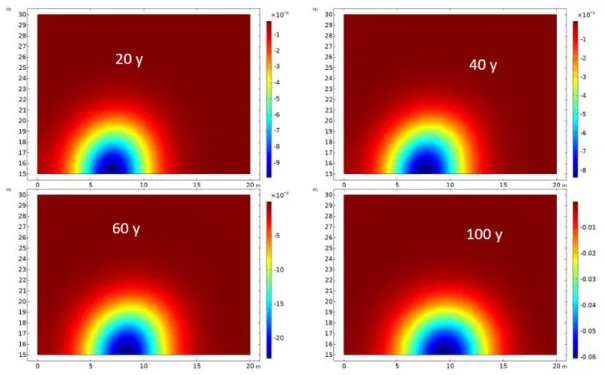
Figure 17 shows the spatial distribution of the vertical displacement at the surface for different moments. We can observe the evolution of subsidence both in its form and in its intensity. The relevance of the numerical model, although simple, coupling dissolution and mechanical response, resides in the time predictive character of the method. Figures. 18 and 19 give some quantitative values of the displacement. From Figure 19 we can observe that the location of the maximum of the subsidence evolves in space when time (dissolution) increases. The position of these points is important in the analysis of the soil-structure interaction and the evaluation of the mechanical consequences on them. The effects on the structure depend among other things on the location and the footprint of the structures (building, railway, bridges, etc.). In the case of dissolution, these relative positions (positions of structures in surface basin) are not constant and evolve with time, due do dissolution. It is therefore interesting to be able to estimate its temporal evolution in order to prevent possible damage of the structures. The proposed method can achieve this goal. Figure 20 depicts a 3D representation of the spatial distribution of the vertical displacement at the surface for different times. We can observe the time evolution of the vertical displacement with the evolution of the lens’s dissolution (boundaries –red circles).
16
Figure. 17. Spatial distribution of the vertical displacement at the surface at t= 20, 40, 60, 100 years.
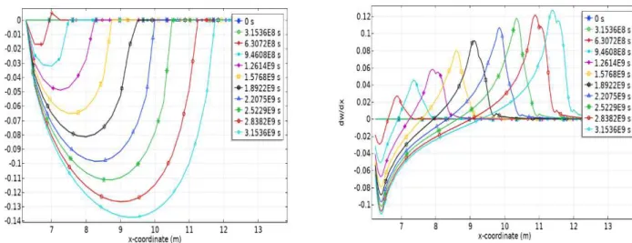
Figure 18. Time (every 10 years) and space evolution of the vertical displacement (left) and the derivative of the vertical displacement with respect to x along line CD (right).
Figure 19. Time (every 10 years) and space evolution of the vertical displacement (left) and the derivative of the vertical displacement with respect to x along line AB (right)
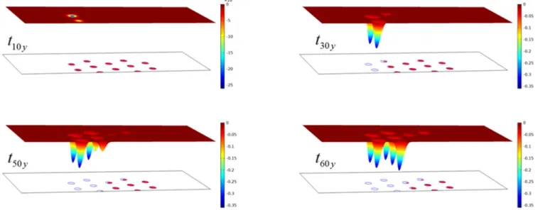
Figure 20. 3D Spatial distribution of the vertical displacement at the surface and state of gypsum (red circle) at t= 10, 30, 50, 60 years.
We see that the subsidence evolves with time and is far from being uniform. It is more significant in upstream than in downstream. The concentration of the fluid increases (from upstream to downstream) while the rate of dissolution decreases. Consequently, the mechanical effects in terms of subsidence on the surface also undergoes this shift over time. A steady state will be reached only if all gypsum is dissolved. Figure 21 illustrates quantitatively this last remark. It depicts the spatial distribution of the normalized concentration on a horizontal cross plane passing through the middle of the lenses and state of gypsum (black circle) for different moments (t= 0, 10, 30, 50, 60 years).
Figure 21. Spatial distribution of the normalized concentration on a horizontal cross plane passing through the middle of the lenses and boundaries of gypsum (black circle) at t= 0, 10, 30, 50, 60 years.
For a more quantitative understanding, we focus on the vertical displacement evolution computed at particular locations of the surface. For this, we consider six points (P1-P6) located on the surface and in the center of six lenses. Figure 22 not only gives the maximum vertical displacement value but also the time required to reach it. We also observe the time difference induced by the flowing of partially saturated fluid and pure water.
17 3.2 2D plane strain - elastoplastic recovery
In this subsection, we discuss the evolution of subsidence as a function of dissolution in plane strain condition. The boundary and initial conditions are depicted in Figure 23. The water level is located at the gypsum layer roof. The gypsum layer is bounded at the top by a soft elastoplastic soil. For this soil an associated Mohr-Coulomb failure is used. It has a Young’s modulus of 100 MPa, a Poisson coefficient of 0.3, a friction angle of 25° and a cohesion equal to 0.04 MPa. The upstream velocity V is 5×10⁻⁷ m/s.
In this case the gypsum has a height of 2 m and is very close to the surface (depth of 7.5 m). Note that in many countries (Toulemont, 1981, 1987) there exists gypsum layer very close to the surface.
Figure 23. 2D plane dissolution-mechanical model (left) and finite element mesh and location of the gypsum lens.
Figure 24. Evolution of dissolution of gypsum layer (in red) and induced effective plastic strain in the recovery
As expected, the faster the dissolution, the more plasticity develops in the soil recovery (Figure 24). The method gives also information on the history of plasticity development within this recovery. The maximum dissolution of the gypsum layer is approximately 12 m. Then there is no longer convergence of the numerical algorithm. If the problem is mathematically well posed, we can attribute the loss of convergence to the loss of soil stability. The soil can no longer support the excess stress generated by the growth of the cavity. This fact is corroborated by the evolution of the subsidence located in the center of the model (Figure 28).
Note that the stability analysis is carried out based on the plastic limit and not on the basis of the second order work criterion (Prunier (2009), Laouafa (2011)). In order to compare the distribution and intensity of the plasticity within the soil layer, we compared that resulted from dissolution and that resulted by carrying out an instantaneous extraction of 12 m of gypsum (Figure 25). The comparison in terms of displacement and slope is depicted in Figure 26.
18
Figure 25. Effective plastic strain in the recovery. Obtained by dissolution (left) and instantaneous extraction (right)
The first remarks that can be made when examining Figure 25 are as follows. The critical void sizes are very similar regardless of the method. It is however difficult, even dangerous, to generalize this result in the case of different geometrical and hydrodynamic configurations. However, a significant difference exists in the spatial distribution of the effective plastic strain. If the recovery is constituted by a more fragile, brittle rock, early damage could give rise to fracturing. Furthermore, if the hydraulic pressure is high then rupture could be reached more quickly in time and space. This mechanism cannot be described by adopting instantaneous excavation. Let us also emphasize that plasticity develops at places but also at given times (results of computation).
Figure 26. Vertical displacement, comparison between dissolution and instantaneous extraction (left). Evolution slope in % during dissolution.
Figure 27 gives the time evolution of the void along the line AB (denoted in Fig. 16) and the location and shape of normalized porosity along AB every 10 years. The S shaped curves are intrinsic to our DIM approach.
Figure 27. Time evolution of the void along line AB (Fig. 16) (left) and normalized porosity (diffuse interface) along AB every 10 years. 1 means fluid and 0 means solid.
Figure 28 depicts the time evolution of vertical displacement of a point located in the surface and the middle of the model. The shape of displacement versus time and the velocity indicate clearly a loss of stability. This kind of collapse may lead to classical sinkholes.
Figure 28. Time evolution vertical displacement (left) and velocity (right) during dissolution process
3.3 Elastoplastic gypsum pillar
The problem considered in this subsection is the isothermal dissolution of a cylindrical gypsum pillar of height 2.5 m and diameter of 5 m (Figure 29). The pillar is located between two supposed non permeable domains (above and below). The imposed upstream flow (inlet)
19
velocity V is equal to 10-6 m/s. The concentration of the dissolving species in the inlet fluid is zero. All the boundaries of the layer containing the lens are zero flux, except for the inlet and the outlet boundaries. The permeability K of the gypsum is 10-15 m2 and that of the surrounding medium is 10-10 m2. The dynamical viscosity of the fluid is that of water (10-3 Pa s). All boundaries of the layer from a mechanical point of view are rollers. The elastoplastic (Mohr-Coulomb) gypsum pillar has a Young's modulus of 35000 MPa, a Poisson coefficient of 0.3, a cohesion of 2000 MPa and a friction angle of 35°. The overburden (height 2 m) is supposed elastic (35000 MPa, a Poisson coefficient of 0.3,). A pressure P equal to 4.8 MPa is applied on the top of the surface.
Figure 29. Gypsum pillar model and boundary conditions (left), mesh and zoom (right)
During continuous injection of fresh water, the dissolution of gypsum pillar is strongly controlled by the concentration of the flowing fluid near the pillar surface. We can observe in Figure 30 the time evolution of the pillar shape and concentration distribution.
Figure 30. Normalized concentration field and shape of gypsum pillar (black) at different times. Values in horizontal plane cross section passing through the middle of the pillar.
Figure 31. Example of streamline and fluid velocity vector field around the pillar at three instants.
Due to the low Reynolds numbers Re (mainly linked to very low fluid velocity), 6 3 1000 10 2.5 Re 2.5 10 V H
ρ
µ
− − × ×= = = the flow is smooth and laminar, and symmetry is
conserved (Figure 31) since no eddies develop behind the cylinder.
Figure 32 shows the plasticity evolution inside the pillar with dissolution. As expected, under a constant external loading, when dissolution increase, plasticity increases. We observe that distribution is not symmetric, but more important at the upstream of the pillar.
Figure 32. Evolution of Plastic deformation in the pillar for three times (15, 18 and 25 years). The black line denotes the initial pillar configuration.
20
The last configuration is the last converged Newton-Raphson solution. When analyzing the displacement history, this non-convergence means collapse of the pillar. The main lesson of this last simulation is that we can predict (under some conditions) the collapse of the pillar (Figures 32 and 33) and eventually its consequence on the stability of the recovery.
Figure 33. Time evolution of the vertical displacement of the material located on top of the pillar
In the above examples (cylindrical gypsum lenses and cylindrical pillar) we see that symmetry of the fluid flow is preserved. We observe also that the rate of dissolution is uniform along the height of theses rocks structures. This is mainly due to the very low fluid velocity and very low Rayleigh number in case of gypsum, which indicates that no natural convection occurs). Figure 34 depicts the shape obtained with ALE method and considering a more soluble pillar rock, halite (salt) for instance. In this purely dissolution problem, we observe a significant change in the final shape of the pillar.
Figure 34. 3D and top views. Example of effect of Rayleigh (Ra) and Reynolds number (Re) on the intensity and on the shape of the dissolution on an initial cylindrical salt pillar.
Recall that: 3 g L Ra D
ρ
µ
∆ = or in porous media Ra g K L Dρ
µ
∆ = and Pe LcV D =In such case the failure mode may be quite different. These cases are under study. In the first modeling we used an isotropic elastoplastic model for gypsum. No mechanical volumetric strain εV was consider affecting in the permeability. In future work we will use a model proposed by Chin et al. (2000) where
(
0)
0 0 1 1 1 V , n eε K K φ φ φ φ = − − = (22) Expression in which n is in the range to 5 to 15, or a more relevant expression of the permeability function of the dissolution process and to the mechanical deformation:( ( , ), V)
K≡K
ε ω ε
t21
4.
Concluding remarks
In this paper, we have discussed the problem of the dissolution of rock materials and rock formations, with a focus on gypsum material. A modeling approach was developed using a weak coupling (impact of dissolution on mechanical behavior) between dissolution and geomechanical behavior. The dissolution model is based on a macro-scale or Darcy-scale model obtained by upscaling the microscopic scale or pore scale equations, using the volume averaging theory, which allows to relate explicitly the form of the macro-scale equations and the effective properties to the pore-scale physics. The application to several problems typically encountered in engineering shows the importance of the rock solubility on the cavity formation and the coupling between transport including dissolution and geomechanics. Numerous theoretical examples treated in this demonstrated the potentialities of the methodology. It must be emphasized that the fields of application of the DIM method are much broader.
The weakly coupled sequential approach for solving dissolution and geomechanics allowed us to obtain already interesting results in terms of risk analysis. Better accuracy, or further applications, would require the introduction of a stronger coupling between geomechanics and dissolution. We expect to integrate in the short term a strong coupling between dissolution and geomechanics, mainly in the context of leaching. In the case of matrix dissolution, work is under way to describe dissolution of multi-scale heterogeneous media. The case of handling heterogeneities, if they cannot be included in the Darcy-scale mesh representation is an open subject, i.e., how to modify the Darcy-scale mathematical model to take into account, let us say, centimetric heterogeneities such as nodules or strata. Work is in progress to achieve this goal.
In such a configuration, another problem for a relevant coupling is the description of the evolution of the mechanical behavior of the material at the material point level. For porous materials, dissolution results in a reduction-modification of the frontiers of the domain but also into a modification of the pore volume. This latter mechanism, depending on its intensity, can radically change the behavior of the material (modulus, yield surface, flow rule, etc.) and pose a difficult challenge for the development of a model. Another point that seems interesting to investigate is dissolution in media with several significantly different characteristic porosity scales. For example, dissolution in fractured media and in the case of double or multiple porosities media.
22
References
Al-Khdheeawi E. A., Vialle S., Barifcani A., Sarmadivaleh M., Iglauer S. (2017a). Impact of reservoir wettability and heterogeneity on CO2-plume migration and trapping capacity.
Int. J. Greenhouse Gas Control, 58:142-158.
Al-Khdheeawi E. A., Vialle S., Barifcani A., Sarmadivaleh M., Iglauer S. (2017b). Influence of CO2-wettability on CO2 migration and trapping capacity in deep saline aquifers.
Greenhouse Gases: Sci. Technol., 7(2):328-338.
Al-Khdheeawi E. A., Vialle S., Barifcani A., Sarmadivaleh M., Iglauer S. (2017c). Influence of rock wettability on CO2 migration and storage capacity in deep saline aquifers. Energy
Procedia, 114:4357-4365.
Al-Khdheeawi E. A., Vialle S., Barifcani A., Sarmadivaleh M., Iglauer S. (2018). Effect of wettability heterogeneity and reservoir temperature on CO2 storage efficiency in deep saline aquifers. Int. J. Greenhouse Gas Control, 68: 216-229.
Anderson D. M., McFadden G. B. (1998). Diffuse-interface methods in fluid mechanics.
Annu. Rev. Fluid Mech., 30: 139–165.
Bell F. G., Stacey T. R., Genske D. D. (2000). Mining subsidence and its effect on the environment: some differing examples. Environ. Geol., 40(1–2): 135–152
Bérest P.,Béraud J. F., Brouard B., Blum P. A., Charpentier J. P., de Greef V., Gharbi H., Valès F.( 2019). Very slow creep tests on salt samples. Rock Mech. Rock Eng., 52: 2917–2934
Brinkman H. C. (1947). A calculation of the viscous force exerted by a flowing fluid on a dense swarm of particles. Appl. Sci. Res., 1: 27–34.
Carter N. L., Horseman S. T., Russell J. E., Handin J. (1993). Rheology of rock salt. J. Struct.
Geol., 15: 1257–1271.
Castellanza R., Gerolymatou E., Nova R. (2008). An attempt to predict the failure time of abandoned mine pillars. Rock Mech. Rock Eng., 41: 377-401
Charmoille A., Daupley X., Laouafa F. (2012). Analyse et modélisation de l'évolution
spatio-temporelle des cavités de dissolution. Report DRS-12-127199-10107A. INERIS
Chin L. Y., Raghavan R., Thomas L. K. (2000). Fully coupled geomechanics and fluid‐flow
23
Collins J. B., Levine H. (1985). Diffuse interface model of diffusion-limited crystal growth.
Phys. Rev. B, 31: 6119–6122.
Cooper A. H. (1988). Subsidence resulting from the dissolution of Permian gypsum in the Ripon area; its relevance to mining and water abstraction. Geological Society, London,
Eng. Geol. Spec. Publ., 5: 387-390
Courtelieris F. A., Delgado J. M. P. Q. (2012). Transport Process in Porous Media. Springer Cristescu N. D., Hunsche U. (1998). Time Effects in Rock Mechanics. Series: Materials,
Modelling and Computation. Wiley, Chichester
Donea J., Giuliani S., Halleux J. P. (1982). An arbitrary Lagrangian-Eulerian finite element method for transient dynamic fluid-structure interactions. Comput. Method Appl. M., 33: 689–723.
Freeze R. A., Cherry J. A. (1979). Groundwater. Prentice-Hall.
Gerolymatou E., Nova. R. (2008). An analysis of chamber filling effects on the remediation of flooded gypsum and anhydrite mines. Rock Mech. Rock Eng., 41, 403–419
Golfier F., Zarcone C., Bazin B., Lenormand R., Lasseux D., Quintard, M. (2002). On the ability of a Darcy scale model to capture wormhole formation during the dissolution of a porous medium. J. Fluid Mech., 457: 213–254.
Guo J., Quintard M., Laouafa F. (2015). Dispersion in porous media with heterogeneous nonlinear reactions. Transp. Porous Media, 109: 541–570
Guo J., Laouafa F., Quintard M. (2016). A theoretical and numerical framework for modeling gypsum cavity dissolution. Int. J. Numer. Anal. Meth. Geomech., 40: 1662–1689.
Gysel M. (2002). Anhydrite dissolution phenomena: Three case histories of anhydrite karst caused by water tunnel operation. Rock Mech. Rock Eng., 35: 1–21
Iglauer S. (2017) CO2–Water–Rock wettability: Variability, influencing factors, and Implications for CO2 Geostorage. Acc. Chem. Res., 50(5): 1134-1142.
James A. N., Lupton A. R. R. (1978). Gypsum and anhydrite, in foundations of hydraulic structures. Geotechnique, 28: 249-272.
Jeschke A. A., Dreybrodt W. (2002) Dissolution rates of minerals and their relation to surface morphology. Geochim. Cosmochim. Acta, 66, 3055– 3062.,
Jeschke A. A., Vosbeck K., Dreybrodt W. (2001). Surface controlled dissolution rates of gypsum in aqueous solutions exhibit nonlinear dissolution kinetics. Geochim.
24
Laouafa F., Prunier F., Daouadji A., AlGali, H., Darve F. (2011). Stability in geomechanics, experimental and numerical analyses. Int. J. Numer. Anal. Meth. Geomech., 35: 112–139 Luo H., Quintard M., Debenest G., Laouafa F. (2012). Properties of a diffuse interface model
based on a porous medium theory for solid-liquid dissolution problems. Comput.
Geosci., 16(4): 913-932
Luo H., Laouafa F., Debenest G., Quintard M. (2015). Large scale cavity dissolution: From the physical problem to its numerical solution. Eur. J. Mech. B-Fluid, 52: 131–146 Luo H., Laouafa F., Guo J., Quintard M. (2014) Numerical modeling of three-phase
dissolution of underground cavities using a diffuse interface model. Int. J. Numer. Anal.
Meth. Geomech., 38: 1600–1616.
Prunier, F., Laouafa, F., Darve, F. (2009). 3D bifurcation analysis in geomaterials investigation of the second order work criterion. Eur. J. Environ. Civ. Eng., 13(2): 135-147
Quintard M., Whitaker S. (1994). Transport in ordered and disordered porous media 1: The cellular average and the use of weighing functions. Transp. Porous Media, 14: 163–177. Quintard M., Whitaker S. (1994). Convection, dispersion, and interfacial transport of
contaminant: Homogeneous porous media. Adv. Water Resour., 17: 221–239.
Quintard M., Whitaker S. (1999). Dissolution of an immobile phase during flow in porous media. Ind. Eng. Chem. Res., 38: 833–844.
Toulemont M. (1987). Les risques d’instabilité liés au karst gypseux lutétien de la région parisienne – Prévision en cartographie. Bull. de liaison P. et Ch., 3192:109-116.
Toulemont M. (1981). Evolution actuelle des massifs gypseux par lessivage. Cas des gypses Lutétiens de la région parisienne, France. Bulletin de liaison. Laboratoire régional des
Ponts et Chaussées de l'Est parisien, France.
Sadeghiamirshahidi M., Vitton S. J. (2019). Laboratory study of gypsum dissolution rates for an abandoned underground Mine. Rock Mech. Rock Eng., 52: 2053–2066
Shovkun I., Espinoza D. N. (2019). Fracture propagation in heterogeneous porous media: Pore-scale implications of mineral dissolution. Rock Mech. Rock Eng., 52: 3197–3211 Swift G. M., Reddish D. (2002). Stability problems associated with an abandoned ironstone
mine. Bull. Eng. Geol. Env., 61: 227–239
25
Van Everdingen, R.O. (1981). Morphology, hydrology and hydrochemistry of karst in
permafrost near Great Bear Lake, Northwest Territories, Paper 11. National
Hydrological Research Institute of Canada.
Wang L., Bérest P., Brouard B. (2015). Mechanical behavior of salt caverns: Closed-form solutions vs numerical computations. Rock Mech. Rock Eng., 48: 2369–2382
Waltham T., Bell F., Culshaw M. (2005). Sinkholes and Subsidence. Karst and Cavernous
Rocks in Engineering and Construction. Springer-Verlag.
26
Figure 1. Land subsidence (sinkhole) in Central Kansas related to underground rock dissolution (after USGS water science).
27
Figure 3. Original dissolution model (sharp interface on the left) and Diffuse Interface Model (on the right).
Figure 4: Large-scale (left) and near interface scale (right)
Figure 5. Averaging volume at pore scale level and material point position vector (left) and 3-phases model (the third phase may be insoluble species for instance) (right).
28
Figure 6. Examples of various 1D, 2D and 3D unit cells (after Courtelieris and Delgado (2012))
29
Figure 8. Views of a pillar in the Rocquevaire abandoned quarry (Bouches-du-Rhône, France) with two different water flooding levels (at two different times 1996 and 2010, by courtesy of Watelet JM, INERIS) and (right) schematic section through a hidden void found within cover rocks of gypsum in Paris (France) railway station underground (After Toulemont (1987)).
Figure 9. Examples of dissolution consequences: (Left) several sinkholes in wood Buffalo National Park (Canada). An interstratal dissolution of gypsum induce a collapse that propagates through dolomite cover beds and (right) (after Walthan et al. (1981), Van Everdingen (1981))
30
Figure 10. Mesh and location of soluble gypsum lens and water level.
31
Figure 12. Time evolution of a cross section passing through the middle of the cylindrical lens, with the contours corresponding to time of 0, 20, 30, 40, 50, 60 and 65 years, respectively.
Figure 13. Effective plastic strain distribution in the recovery after 20, 40, and 60 years (top) and isovalues of the effective plastic strain distribution in the recovery after 20, 40, and 60 years.
32
Figure 14. Time evolution of the volume integration of the effective plastic strain over the overburden.
Figure 15. 3D distribution of vertical displacement when the gypsum lens is totally dissolved (left) and vertical displacement w(t) as function of time at two points A and B (right).
33
Figure 16. Geometrical model used for the subsidence analysis. Single gypsum lens (top) and multiple gypsum lenses (bottom).
Figure 17. Spatial distribution of the vertical displacement at the surface at t= 20, 40, 60, 100 years.
34
Figure 18. Time (every 10 years) and space evolution of the vertical displacement (left) and the derivative of the vertical displacement with respect to x along line CD (right).
Figure 19. Time (every 10 years) and space evolution of the vertical displacement (left) and the derivative of the vertical displacement with respect to x along line AB (right)
35
Figure 20. 3D Spatial distribution of the vertical displacement at the surface and state of gypsum (red circle) at t= 10, 30, 50, 60 years.
Figure 21. Spatial distribution of the normalized concentration on a horizontal cross plane passing through the middle of the lenses and state of gypsum (black circle) at t= 0, 10, 30, 50, 60 years.
36
Figure 22. Location of six points P1-P6 (left) and their vertical displacement (right)
Figure 23. 2D plane dissolution-mechanical model (left) and finite element mesh and location of the gypsum lens
37
Figure 24. Evolution of dissolution of gypsum layer (in red) and induced effective plastic strain in the recovery
Figure 25. Effective plastic strain in the recovery. Obtained by dissolution (left) and instantaneous extraction (right)
38
Figure 26. Vertical displacement, comparison: dissolution vs instantaneous (left). Evolution slope in % during dissolution.
Figure 27. Time evolution of the void along line AB (Figure 16) (left) and normalized porosity (diffuse interface) along AB every 10 years. 1 mean fluid and 0 solid.
39
Figure 28. Time evolution vertical displacement (left) and velocity (right) during dissolution process
40
Figure 30. Normalized concentration field and shape of gypsum pillar (black) at different times. Values in horizontal plane cross section passing through the middle of the pillar.
Figure 31. Example of streamline and fluid velocity vector field around the pillar at three instants.
41
Figure 32. Evolution of Plastic deformation in the pillar for three times (15, 18 and 25 years). The black line denotes the initial pillar configuration.
Figure 33. Time evolution of the vertical displacement of the material located on top of the Pillar
15
t
=
y
t
=
18
y
20
42
Figure 34. 3D and top views. Example of effect of Rayleigh (Ra) and Reynolds number (Re) on the intensity and on the shape of the dissolution on an initial cylindrical salt pillar.