Capacity planning with demand uncertainty for outpatient clinics
The MIT Faculty has made this article openly available. Please sharehow this access benefits you. Your story matters.
Citation Nguyen, Thu Ba T et al. "Capacity planning with demand uncertainty for outpatient clinics." European Journal of Operational Research 267, 1 (May 2018): 338-348 © 2017 Elsevier
As Published http://dx.doi.org/10.1016/j.ejor.2017.11.038
Publisher Elsevier BV
Version Author's final manuscript
Citable link https://hdl.handle.net/1721.1/122356
Terms of Use Creative Commons Attribution-NonCommercial-NoDerivs License
1
CAPACITY PLANNING WITH DEMAND UNCERTAINTY FOR
OUTPATIENT CLINICS
Thu Ba T. NGUYEN1, Appa Iyer SIVAKUMAR2, Stephen C. GRAVES3
1Southampton Business School, University of Southampton
University Road, Southampton, SO17 1BJ, United Kingdom E-mail: [email protected]; [email protected]
2School of Mechanical and Aerospace Engineering, Nanyang Technological University
50 Nanyang Avenue, Singapore 639798 Email: [email protected]
3Sloan School of Management, Massachusetts Institute of Technology
77 Massachusetts Avenue, Cambridge, Massachusetts 02139, USA Email: [email protected]
Abstract
In this study we develop a capacity planning model to determine the required number of physicians for an outpatient system with patient reentry. First-visit (FV) patients are assumed to arrive randomly to the system. After their first appointment, the FV patient may require additional appointments, and will then become a re-visit (RV) patient; after each appointment an RV patient will require subsequent visits with a given probability. The system must achieve a set of targets on the appointment lead-times for both FV and RV patients. Furthermore, the system must have sufficient capacity to assure that a given percentile of FV patients is admitted. We develop a deterministic model that finds the required capacity over a finite horizon. We establish the tractability of the deterministic model and show that it provides a reasonable approximation to the stochastic model. We also demonstrate the value from knowing the demands in terms of the required resources. These conclusions are numerically illustrated using real data from the Urology outpatient clinic of the studied hospital.
Key words: OR in health services, appointment lead-time, capacity planning, demand uncertainty
2 1. Introduction and literature review
The long time for an outpatient to get an appointment has become a crucial concern of the Singapore Ministry of Health (MOH). Thus, the MOH has required its hospitals to maintain better control over its appointment lead-times; in particular, the MOH has set targets for each hospital for the median, 95th percentile, and 100th percentile of the patients’ appointment lead-time. This requirement is particularly challenging for Tan Tock Seng Hospital (TTSH) (e.g., Urology specialty), which is a government hospital, due to the re-entry characteristics (Nguyen et al., 2015) of the admitted patients. After each visit, the physician decides whether a return visit is warranted for the patient, and if so, then prescribes the return interval (e.g., come back in three to four weeks) and the length of his/her appointment (the length of the return appointment is shorter than that of the first appointment in TTSH’s Urology clinic). Although the hospital has made improvements in mitigating and reducing the no-show rate, it has struggled in its efforts to meet the MOH appointment lead-time targets. Hospital managers and physicians have identified inadequate planned capacity as being a crucial source for both the long appointment delays, as well as the unacceptable level of patients’ requests that cannot be accommodated within the normal clinic schedule. These latter requests are termed to be rejected, and the patients are sent to an open session for the clinic. Thus, there is a need for an improved approach for capacity planning so as to improve the system’s performance as well as to meet the MOH targets on patients’ appointment lead-time. This study determines how many physicians are needed to serve the uncertain patient demand accounting for both the appointment lead-time targets and the patient re-entry.
Capacity planning for outpatient appointment systems, as evidenced within TTSH, has been a challenge and interesting field to many researchers (Ahmadi-Javid et al., 2016). Previous research has taken different approaches to determine the necessarily planned capacity. Some studies focus on how to allocate the available capacity to the accepted admission requests to optimize the performance measurement. Other studies attempt to determine the capacity that is required to achieve performance targets for a given level of patient arrivals. The former studies are termed as the resource allocation problem, while the latter ones are the capacity design problem.
For the resource allocation problem, Qu et al. (2007), Qu et al. (2011), and Qu et al. (2012) considered how to optimally manage the arrival demands for each type of patients
(walk-3 in and advanced booking patients), so as maximize the number of patients seen. The authors optimized the percentage of appointments held open per session, and developed a mathematical function of the number of patients seen, for different no-show rates. The authors assumed that the arrival distributions are known and the number of scheduled patients is predetermined. Qu et al. (2007) and Qu et al. (2012) investigated a single horizon for the open appointments, while Qu et al. (2011) extended the study for the hybrid time horizons. In addition to increasing the average number of patients, Qu et al. (2012) focused on reducing the variability of patients seen. Saure et al. (2012) investigated a Markov decision process and its equivalent linear programming to allocate patient arrivals to the available capacity. The study addressed the uncertainty of daily arrivals and multiple session duration. The objective is to minimize the costs of patient wait times, of physician overtime, and of postponing some of the booking decisions over a finite planning horizon.
The appointment scheduling problem is another approach for resource allocation. This problem has been studied extensively in the literature; Cayirli and Veral (2003) provided a review of the literature and some recent published papers include Green et al. (2006), Creemers (2012), LaGang and Lawrence (2012), Balasubramanian et al. (2014), Kemper et al. (2014), Kuiper and Mandjes (2015), Patrick et al. (2016), Mak et al. (2016), and Nguyen et al. (2016). The research examines the trade-offs between patient waiting time, and physician idle-time and/or physician over-time. These studies, however, do not explicitly consider the achievement of the appointment lead-time targets, with the exception of Nguyen et al. (2016). However, Nguyen et al. (2016) do not determine how many physicians are needed to achieve the established targets
In addition, some research has explored the integration between the tactical problem of resource allocation and the operational problem of appointment scheduling. Qu et al. (2013) proposed a mixed integer linear program to allocate service categories into clinic sessions during a week for balancing the workload among the sessions. The authors use a stochastic mixed integer program to determine the optimal number of appointments for each service type in each session to minimize a weighted sum of patient waiting time, provider idle time, and provider overtime in each clinic session. Cayirli and Gunes (2014) integrated the capacity and appointment decisions to minimize the total patient waiting time, physician idle time and overtime. The study determined the capacity to reserve for walk-in patients versus advanced
4 booking. Liu (2016) investigated a queueing model for setting the appointment scheduling window (which is equivalent to the appointment lead-time definition) in light of patient no-show behavior. The study controlled the queue capacity in order to maximize the expected revenue. The restriction of patients’ appointment lead-time/s was not addressed.
For the capacity design problem, Ozcan (2005) introduced queueing models to determine service capacities or the number of physicians. The models highlight the relationships between average patient waiting time, physician idle-time, and physician over-time. Leithch et al. (1990), Bennett and Worthington (1998), Porta-Sales et al. (2005), Bamford and Chatziaslan (2009), and Demir et al. (2012) examined the required capacity from predicting the demands. Leitch et al. (1990) used an empirical analysis to determine follow-up demands. A part of the study in Bennett and Worthington (1998) addressed a simple spreadsheet calculation to simulate the additional required capacity assuming a positive correlation between the number of appointments saved and the length of patients’ mean appointment lead-time. Porta-Sales et al. (2005) identified reasons of follow-up non-compliance such as becoming an inpatient, or passing away, or following-up somewhere else. The authors proposed an equation to predict non-compliance. As the result, the predicted requirement of capacity is more accurate due to reduced non-compliance. Bamford and Chatziaslan (2009) introduced a survey method to measure capacity at the operational level, which considers the variation of available capacity throughout a year. From the finding, the human resource department can plan the required personnel to match the demand. Demir et al. (2012) suggested a model to predict a future demand, assuming that the demand linearly increases with time. The authors considered both independent and dependent demands between specialties.
Likewise, Ittig (1985), Worthington (1991), Street and Duckett (1996), Thomas et al. (2001), Bowers et al. (2005), Qu and Shi (2009), Elkhuizen et al. (2007), Green and Savin (2008), Bowers (2010) proposed different methods to find the required capacity. Ittig (1985) used a linear programming model to maximize profit while considering both linearly and exponentially dependent appointment lead-times. The capacity level depends on the arrivals, which is a function of appointment lead-times. Worthington (1991) used a projection method to evaluate different capacity planning alternatives considering patient behavior. The goal of the study is to predict the future waiting list size as well as the mean appointment lead-time. The author restricted the appointment lead-times for follow-up based on the priority of patient
5 groups. In Street and Duckett (1996), an empirical study revealed that the payment policy has an impact on the waiting list.
Thomas et al. (2001), Bowers et al. (2005), Qu and Shi (2009) provided analytical methods to determine the capacity level. In Thomas et al. (2001), the surplus capacity to avoid long appointment lead-time of patients was determined from a mean number of arrivals and a percentage of patients who will be seen within the lead-time targets. Bowers et al. (2005) calculated the number of clinics required in each specialty from information on demand arrivals, no-show rates, and an expected utilization of the clinic. In the study, the authors considered follow-up rates in which patients come back as revisit patients only one time. Qu and Shi (2009) determined the expected number of scheduled patients and the variance of the number of consulted patients from demands and no-show rates for two different types of patients (walk-in and advanced booking patients).
Elkhuizen et al. (2007) used a simulation approach to predict the capacity level for a mean and 95th percentile of patients’ appointment lead-time. Green and Savin (2008) applied a queuing model to determine a capacity requirement for the same-day appointment system. The study focused on identifying an appropriate compromise between the physician capacity level and patient backlog. Bowers (2010) proposed a predictive model for determining the additional resources required. The author aimed to provide a better intuition of information needed to achieve the targets of patients’ appointment lead-time.
Although Leitch et al. (1990), Porta-Sales et al. (2005), Bowers et al. (2005) considered follow-up demands in their studies, only Bowers et al. (2005) provided a quantitative method to plan capacity. However, Bowers assumed that the patients return only once. This assumption may cause an under-estimation of the required capacity for the re-entry system in which the patients need multiple returns to the system. Neither Leitch et al. (1990), Porta-Sales et al. (2005) nor Bowers et al. (2005) investigated the patients’ appointment lead-time. The patients’ appointment lead-time was considered in Ittig (1985), Worthington (1991), Bennett and Worthington (1998), Thomas et al. (2001), Elkhuizen et al. (2007), Bowers (2010). The studies of Ittig (1985), Thomas et al. (2001), Elkhuizen et al. (2007) considered an appointment lead-time for non-reentry system; Worthington (1991), Bennett and Worthington (1998), and Bowers (2010) allowed for re-entry patients. However, Bennett and Worthington (1998) focused on the appointment lead-times of follow-up cases in clinics for which the number of routine
6 appointments per year reflects a stable situation. Worthington (1991) and Bowers (2010) did not provide a quantitative calculation for the required capacity. In general, these papers provide some significant insights for planning capacity, but they are not readily applicable for a re-entry clinic that needs to satisfy multiple patients’ appointment lead-time targets.
In Nguyen et al. (2015), we presented a linear optimization model to plan the physician requirement with consideration of multiple-appointment lead-time targets. Furthermore, we included the assurance of the continuity of care for the follow-up patients in our model. The study minimizes the maximum required capacity and determines how to allocate the required resources between new arrival and follow-up demands. The paper assumed that all requests must be admitted, and assumed known, deterministic arrivals. In the current paper we relax the assumption of deterministic arrivals. We now summarize the major contributions of the present work:
a. We extend the deterministic linear optimization model of Nguyen et al. (2015) to consider uncertainty of the new arrivals. We formulate a stochastic linear optimization model with chance constraints to address the uncertain demands.
b. We derive deterministic equivalents for the stochastic linear optimization model for two cases, depending on the assumed extent of the distributional information of the new arrivals. To do this, we need to specify the “violation risk,” namely the maximum probability that a patient’s request would be denied, denoted as(𝜀).
c. We experimentally compare the deterministic equivalents for the stochastic linear optimization model and determine a robust optimal capacity plan.
This paper is organized as follows. We formulate the stochastic linear optimization model with the maximum risk of violation in Section 2. Section 3 presents the deterministic equivalents of the stochastic problem. In Section 4, we report on numerical experiments; we also analyze the characteristics of the objective and the appointment lead-time targets. Subsequently, we discuss our findings and conclusions in Section 5.
2. Problem development
The development of the following stochastic linear programming model for minimizing the maximum required capacity follows that of Nguyen et al. (2015); thus it is slightly abbreviated. Let u, v, and w be the median, pth percentile, and 100th percentile of first-visit (FV) patients’
7 appointment lead-time targets where: 𝑢 < 𝑣 < 𝑤, and 50 < 𝑝 < 100. In addition, [𝑎, 𝑏] and 𝑎 denote the restricted range of the re-visit (RV) patients’ appointment lead-time and the mean RV patients’ appointment lead-time where: 𝑎 < 𝑎 < 𝑏.
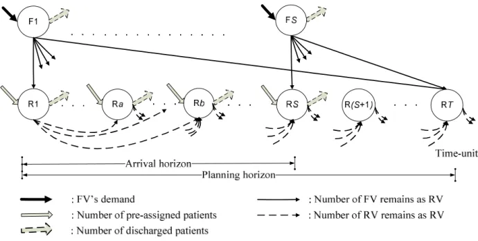
Figure 1: A network flow model for planning capacity of a re-entry appointment system (Nguyen et al., 2015)
We plan for an arrival horizon of S time-units over which FV patients can arrive. However, in order to schedule all patients that arrive within the arrival horizon, we need to extend the planning horizon to be 𝑇 = 𝑚𝑎𝑥(𝑆 + 𝑤, 𝑆 + 𝑏), where w is longest allowable FV appointment lead-time and b is the longest RV lead-time. Figure 1 illustrates a network flow of T time-units of the planning horizon which involves S time-units of the arrival horizon for the FV patients. The FV-nodes are denoted F1, F2, up to FS, for modeling the arrival flow of FV patients; the RV nodes model the scheduling of RV patients and are numbered R1, R2, up to RT.
The black thick arrows that go into the FV-nodes represent the stochastic arrivals of the FV patient 𝑓 at time-unit i. The grey solid arrows that go into the RV-nodes represent the total number of pre-assigned (i.e., previously scheduled) FV patients 𝑟 and RV patients 𝑟 ,
8 respectively. These are the patients whose next appointments are within the arrival horizon, and that were scheduled before the first time period in the model.
List of notation:
𝑢, 𝑣, 𝑤 : Appointment lead-time targets for median, pth percentile, and 100th percentile
respectively, time-units.
𝑝 : The pth percentile (50 < 𝑝 < 100).
[𝑎, 𝑏] : The restricted appointment lead-time of RV patients.
𝑎 : The mean RV patients’ appointment lead-time (𝑎 < 𝑎 < 𝑏), time-units.
𝛼, 𝛽 The constant discharge rates for FV and RV patients, respectively; where 0 < 𝛼, 𝛽 < 1 𝜏 , 𝜏 : The consultation time for FV and RV patients
𝑟 , 𝑟 : Total number of pre-assigned FV patients and RV patients in time-unit j. 𝑓 : The stochastic arrivals of the FV patient in time-unit i.
𝑑 : The total number of RV discharges after their appointment in time-unit j.
𝑥 : The number of FV patients who arrive in the ith time-unit and have appointment in the jth time-unit, and still remain in the system as RV patients after their appointment in the
jth time-unit.
𝑦 : The number of patients who have an appointment in the ith time-unit and have their
next appointment in the jth time-unit, and still remain as RV patients after the jth time-unit.
𝑧 : The number of FV patients who arrive in time-unit i and are assigned appointment in time-unit j.
𝑐 : The total required capacity in time-unit i.
𝑐 , 𝑐 : The required capacity for FV patients and RV patients in time-unit i. S : The number of time-units in the arrival horizon.
T : The number of time-units in the planning horizon, 𝑇 = 𝑀𝑎𝑥(𝑆 + 𝑏, 𝑆 + 𝑤). 𝐿 , 𝐿 : The set of all 𝑧 that satisfy the median (u) and pth percentile (v) lead-time targets.
𝑁 ,𝑁 , 𝑁 : The index set in which 𝑁 = {1, 2, … , 𝑆}, 𝑁 = {𝑆 + 1, 𝑆 + 2, … , 𝑇}, and 𝑁 = 𝑁 ∪ 𝑁
𝜀 : A risk of violation.
Pr(A) : The probability of an event A.
𝐹 ( ) : The cumulative distribution function (CDF) of 𝑓 . 𝜇 , 𝜎 : The mean and variance of the uncertain arrivals, 𝑓 .
9 The thick arrows that go out from FV-nodes represent the total number of FV discharges, who make a request in time-unit i. The thick arrows that go out from RV-nodes illustrate the total number of RV discharges 𝑑 after their next appointment. The time until the next appointment will be between a to b time-units from their current appointment in time-unit j.
The thin solid lines that connect FV-nodes and RV-nodes represent the FV patients that remain as RV patients after their consultation. We use 𝑧 to denote the number of FV patients who make their request in time-unit i and are assigned appointment in time-unit j, where i ; j we then use 𝑥 to denote the FV patients that remain as RV patients after their initial consultation. We let 𝑦 denote the number of RV patients with appointments in time-unit i, who will still remain as RV patients after their subsequent appointment in time-unit j; this is signified by the dashed arrows between RV nodes.
To simplify the model, we assume constant discharge rate 𝛼, 𝛽 for FV and RV patients, respectively where: 0 < 𝛼, 𝛽 < 1. In addition, the model assumes a constant consultation time 𝜏 , 𝜏 for FV and RV patients. The consultation times of patients are measured in minutes.
The model will determine the maximum required capacity, defined as
1 max i i T q c
where 𝑐 is the total required capacity in time-unit i. The total required capacity 𝑐 includes the required capacity for FV patients 𝑐 and RV patients (𝑐 ) in time-unit i, which is measured in minutes. Given the intent to use the model at the tactical level, we assume that all patients will arrive and each physician works the same hours. From the maximum required capacity, q, we can determine the number of full-time equivalent physicians.
As stated earlier, we wish to determine the capacity required to admit all the patients’ request. However, this may require an unreasonable level of capacity, as the future demand of the FV patients is unknown. Hence we restate this service objective in terms of a risk of violation(𝜀); that is, the requirement is that the probability that not all patients’ requests are satisfied is no more than 𝜀. Therefore, the objective of the model becomes to find the minimum required capacity that will achieve the lead-time targets for a given risk of violation.
Finally, we define the sets m
| 0
ij
L z j i u and p
| 0
ij
L z j i v . That is, 𝐿 is the set of all 𝑧 that satisfy the median lead-time target and L is the set of all 𝑧 that satisfy p
10 2, … , 𝑇}, 𝑁 = 𝑁 ∪ 𝑁 . The mixed integer programming model for the capacity design problem with demand uncertainty (P1) is as follows:
[P1]: Min 𝑞 (1) Subject to: 𝑞 ≥ 𝑐 , ∀ 𝑗 ∈ 𝑁, (2) 𝑃𝑟 ∑ 𝑧 ≥ 𝑓 ; ∀𝑖 ∈ 𝑁 ≥ 1 − 𝜀, (3) ∑ 𝑧 = 0; ∀𝑖 ∈ 𝑁 (4) 𝑥 − (1 − 𝛼)𝑧 = 0, ∀𝑖, 𝑗 ∈ 𝑁, (5) 𝑟 + 𝑟 + ∑ 𝑥 + ∑ 𝑦 − 𝑑 + ∑ 𝑦 = 0, ∀𝑗 ∈ 𝑁, (6) 𝑑 − 𝛽 𝑟 + 𝑟 + ∑ 𝑦 + ∑ 𝑥 = 0, ∀𝑗 ∈ 𝑁, (7) 𝑦 = 0, ∀𝑗 − 𝑖 < 𝑎, ∀𝑖, 𝑗 ∈ 𝑁, (8) 𝑦 = 0, ∀𝑗 − 𝑖 > 𝑏, ∀𝑖, 𝑗 ∈ 𝑁, (9) ∑ 𝑑 = 0 , (10) ∑ ∈ 𝑧 ≥ ∑ ∑ 𝑧 + 1, (11) ∑ ∈ 𝑧 ≥ ∑ ∑ 𝑧 (12) 𝑧 = 0, ∀𝑗 − 𝑖 > 𝑤, ∀𝑗 − 𝑖 < 0, (13) ∑ ∑ (𝑗 − 𝑖) 𝑦 − 𝑎 ∑ ∑ 𝑦 ≤ 0, (14) 𝑐 − 𝜏 𝑟 + 𝜏 ∑ 𝑧 = 0, ∀𝑗 ∈ 𝑁, (15) 𝑐 − 𝜏 𝑟 + 𝜏 ∑ 𝑦 = 0, ∀𝑗 ∈ 𝑁, (16) 𝑐 − 𝑐 + 𝑐 = 0 , ∀𝑗 ∈ 𝑁, (17) 𝑥 , 𝑦 , 𝑧 , 𝑐 , 𝑐 , 𝑑 , 𝑑 ≥ 0, ∀𝑖, 𝑗 ∈ 𝑁, (18) 𝑧 ∈ 𝑍 ,∀𝑖, 𝑗 ∈ 𝑁. (19)
Where Pr(A) represents probability of an event A.
The objective (1) minimizes the maximum required capacity, per time-unit, to obtain the established appointment lead-time targets. This maximum required capacity is determined in
11 constraint (2). Constraints (3), (4) and (5) imply the conservation of flow at FV-nodes. Constraint (3) requires that the minimum probability that all patients’ request can be scheduled is(1 − 𝜀). The inequalities on the left hand side of constraint (3) aim to schedule all patients’ request that arrive within the arrival horizon. Furthermore, we observe that constraint (3) is a chance constraint, since the arrivals are random variables 𝑓 ; ∀𝑖 ∈ 𝑁 . Constraint (4) shows that no demands beyond the arrival horizon are considered. Constraint (5) calculates the number of FV patients who will remain as RV patients after their initial consultation.
The conservation of flow at RV-nodes is shown in constraints (6) and (7). The first bracket of constraint (6) shows the inbound flows of all appointments in time-unit j, which includes the total number of pre-assigned FV and RV patients, the total number of FV patients, and the total number of RV patients. The second bracket of constraint (6) illustrates the outbound flows of all appointments scheduled for time-unit j, which involves the number of RV patients discharged after their visit in time unit j, and the number of RV patients remaining with a next appointment. Constraint (7) determines the number of discharged patients after their visit in time-unit j.
Constraint (8) and (9) requires that all RV patients will have appointment lead-times within the restricted range[𝑎, 𝑏]. Constraint (10) states that no RV discharges can be made after the last date of the arrival horizon S. Constraints (11), (12), and (13) specify the achievement of the median, pth percentile, and 100th percentile appointment lead-time target as compulsory, respectively. The restriction of the RV mean appointment lead-time is shown in constraint (14). The required capacities of FV and RV patients in time-unit j are calculated in constraints (15) and (16); and the total required capacity, in time-unit j, is found in constraint (17). The required capacity for either FV or RV patients includes the required capacity of pre-assigned patients and that of the new arrivals. Constraints (18) and (19) give the requirement of non-negative variables and integrality.
3. Approximations of the planning model
Charnes and Cooper (1963) were pioneers in developing the use of chance constraints as a way to handle random variables within an optimization. Their paper shows how to create deterministic equivalents for chance constraints, assuming that the uncertainty follows normal distribution. Calafiore and Ghaoui (2006) derived a tractable deterministic equivalent of a single
12 chance constraint, without any distributional assumptions. The approximation is in the form of a second order cone representation regardless of the distributional information of the uncertainty. Joint chance constraints were further investigated in Nemirovski and Shapiro (2006). They decompose the joint chance constraints into a set of single chance constraints, each of which can be converted into the deterministic equivalents in Calafiore and Ghaoui (2006). Then, the deterministic equivalent constraints provide a conservative approximation of the joint chance constraints problem.
These papers inspire our development of a deterministic equivalent model for capacity planning. We develop a convex approximation of the joint-chance-constraint problem (P1) and then reformulate it as a deterministic linear program. We develop the approximation by decomposing the joint chance constraint (3) of problem (P1) into a set of individual chance constraints. The decomposition relies on a union bound or Boole’s inequality: 𝑃𝑟(∪ 𝐴 ) ≤ ∑ 𝑃𝑟(𝐴 ) (Ross, 1993). The inequality states that the probability that at least one of the events happens is not greater than the sum of the probability of the individual events.
The joint chance constraint (3) bounds the probability that all FV patients are scheduled in all periods. We can reformulate (3) using the intersection of the inequalities as shown in constraint (20):
𝑃𝑟 ∩∈ ∑ 𝑧 − 𝑓 ≥ 0 ≥ 1 − 𝜀. (20)
We rewrite (20) by using 𝑃𝑟(∩ 𝐴 ) = 1 − 𝑃𝑟(∪ (𝐴 ) ), where (𝐴 ) is a complement of 𝐴 : 1 − 𝑃𝑟 ∪∈ ∑ 𝑧 − 𝑓 ≥ 0 ≥ 1 − 𝜀. Thus, the chance constraint (20) is equivalent to constraint (21):
𝑃𝑟 ∪∈ ∑ 𝑧 − 𝑓 < 0 ≤ 𝜀. (21)
In words, constraint (21) sets an upper bound on the probability that there is a violation in one or more time periods, where a violation occurs if we cannot schedule the FV patients. By using a union bound or Boole’s inequality for the constraint (21), we can obtain a bound on the left-hand-side of (21):
𝑃𝑟 ∪∈ ∑ 𝑧 − 𝑓 < 0 ≤ ∑∈ 𝑃𝑟 ∑ 𝑧 − 𝑓 < 0 . (22) Given 𝑃𝑟 ∑ 𝑧 − 𝑓 < 0 ≤ 𝜀 and ∑∈ 𝜀 ≤ 𝜀, we propose to use the following individual chance constraints as a conservative approximation of the constraints (3).
13 where the right-hand-side values
i 0are chosen so that ∑∈ 𝜀 = 𝜀. It is easy to argue, using (22), that constraint (23) assures that (21) is satisfied. We can rewrite (23) as:𝑃𝑟 𝑓 − ∑ 𝑧 ≤ 0 ≥ 1 − 𝜀 , 𝑖 ∈ 𝑁 . (24)
Thus, in (24) we have a lower bound on the probability that we can schedule the FV patients in each period. We propose to fix the values of 𝜀 as 𝜀 = (refer to Nemirovski and Shapiro, 2006). Then, the chance constraints become:
𝑃𝑟 𝑓 − ∑ 𝑧 ≤ 0 ≥ 1 − , 𝑖 ∈ 𝑁 . (25)
We have shown here how to decompose the original chance constraint (3) into a set of individual chance constraints that are tighter than the original constraint (3) in the problem (P1). In the next section, we will determine the deterministic equivalent of these individual chance constraints, which will depend on what is known about the probability distributions.
3.1. Deterministic equivalent for a fully distributional information of the uncertain arrival demands
In this section we assume that we know the probability distribution of the uncertain arrival demands 𝑓 in each period. For instance, we might assume that the arrival demand is normally distributed with known mean and variance. We denote the cumulative distribution function (CDF) of 𝑓 as 𝐹 ( ). Then, the constraint (25) can be rewritten as in constraint (26):
𝐹 ∑ 𝑧 ≥ 1 − , 𝑖 ∈ 𝑁 . (26)
We can transform (26) into linear constraints, by using the inverse of the CDF:
∑ 𝑧 ≥ 𝐹 1 − , 𝑖 ∈ 𝑁 . (27)
We replace the chance constraint (3) in (P1) with (27) to obtain a tractable linear optimization problem, given as follows:
[P1-a]:
Min 𝑞 (1a)
Subject to:
14
∑ 𝑧 ≥ 𝐹 1 − , 𝑖 ∈ 𝑁 , (3a)
Constraints (4) - (19). (4a)
3.2. Deterministic equivalent for a partially distributional information of the uncertain arrival demands
In this section, we provide a second reformulation of (P1) under the assumption that we only have partial distributional information on the arrival demands. We assume that for each period we know the mean (𝜇 ) and variance (𝜎 ) of the arrival demand 𝑓 , but we do not know the distribution. We show in the appendix B, using Chebyshev’s inequality, that we can replace the set of individual constraints (25) with the following set of constraints:
∑ 𝑧 ≥ 𝜇 + 𝜎 , ∀ 𝑖 ∈ 𝑁 (28)
We note that these are now linear constraints, which are tighter than the constraint (25). We can now re-express (P1) by replacing the chance constraint (3) with (28):
[P1-b]: Min 𝑞 (1b) Subject to: 𝑞 ≥ 𝑐 , ∀ 𝑗 ∈ 𝑁, (2b) ∑ 𝑧 ≥ 𝜇 + 𝜎 , 𝑖 ∈ 𝑁 , (3b) Constraints (4) – (19). (4b) 4. Numerical experiments
In this section, we report on our numerical experiments. The intent is to illustrate the impact of assumptions of the uncertain demand on performance, and the advantages of the proposed approximations. The performance measurement is the maximum required capacity.
15 4.1. Experimental design
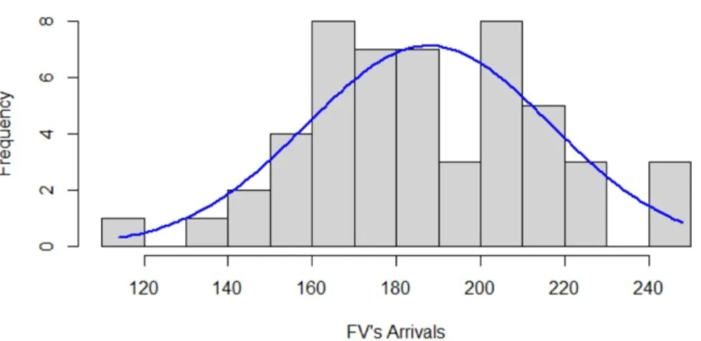
The experiments are implemented with year 2009 as the arrival horizon. The input data were obtained from the Urology specialty in the studied hospital. The data includes the assigned FV and RV patients as of the start of the year 2009; the total number of FV and RV pre-assigned patients are 1,277 and 10,970 patients, respectively. We assumed that weekly arrivals of the FV patients to be from either a normal distribution or an unknown distribution (Figure 2) with given mean and standard deviation. The mean and standard deviation are based on the actual FV arrivals in year 2009, and are equal to 187.7 and 29 arrivals per week, respectively. The observed FV and RV discharge rates of year 2009 are used in the numerical experiments (𝛼 = 0.38, 𝛽 = 0.32).
Figure 2: Normal distribution of the FV’s arrivals for the studied horizon in 2009
Furthermore, the FV targets from the MOH for the median(𝑢 = 2 𝑤𝑒𝑒𝑘𝑠 ), 95th percentile(𝑣 = 6 𝑤𝑒𝑒𝑘𝑠), and 100th percentile (𝑤 = 9 𝑤𝑒𝑒𝑘𝑠 ) appointment lead-time are also needed. The range of the RV appointment lead-time (𝑎 = 2 𝑤𝑒𝑒𝑘𝑠, 𝑏 = 30 𝑤𝑒𝑒𝑘𝑠) and the length of the RV mean appointment lead-time (𝑎 = 16 𝑤𝑒𝑒𝑘𝑠 ) were given by physicians. We set up the model to plan required capacity on a weekly basis. The risk of violation (𝜀) needs to be set as well. We consider 6 different levels of the risk of violation, ε = {0.01; 0.05; 0.10; 0.20; 0.30; 0.40}, to investigate the impact of the violation risk on the optimal required capacity, expressed as the number of full-time equivalent physicians per week. The consultation time for FV and RV patients is 15 and 10 minutes per patient, respectively.
16 We select the Branch and Cut algorithm (Bertsimas and Tsitsiklis, 1997) to solve the problem. The optimal solutions to all the numerical experiments can be obtained in about 4 minutes, implemented in IBM ILOG CPLEX Optimization Studio V12.4 on HP Pavilion G6 Notebook 1.9GHz PC with the Windows 7 operating system.
4.2. Experimental results
Given the inputs described in Section 4.1, Figures 3, 4 and 5 compare the performance between the normal and the unknown distribution approaches, in terms of the maximum and the mean of full-time equivalent physicians for the total number of FV and RV, for only the number of FV, and only the number of RV cases. The maximum values come from solving either a) or (P1-b). The mean values represent the average requirement for full-time equivalent physicians per week over the planning horizon. The number of full-time equivalent physicians per week is calculated from total number of hours required to serve the requests during a week. We assume that a defined physician works 8 hours per week in a clinic.
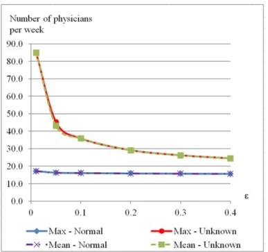
Figure 3: The total number of full-time equivalent physicians required for the normal and unknown distributions at different levels of violation risk.
17 The comparison for the case with all FV and RV patients (Figure 3) shows that the increase of the violation risk (𝜀) reduces the required capacity. This pattern is consistent for both maximum and mean measurements. Furthermore, knowing the distributional information of the arrivals (i.e., normal distribution) may significantly reduce the number of planned resources for either the maximum or the mean required capacity; for example, given 𝜀 = 0.01, the maximum number of required physicians with an unknown distribution is 85 full-time equivalent physicians per week (4,077 slots per week, where each slot is a ten-minute appointment), compared to only 17.2 full-time equivalent physicians per week (825 slots per week) with the normal distribution.
Table 1: Percentage of time periods that only FV, only RV, and mixed patients are served Violation risk Only FV Only RV Both FV and RV
Unknown 0.01 7.3 12.2 80.5 0.05 6.1 13.4 80.5 0.1 6.1 13.4 80.5 0.2 4.9 17.1 78.0 0.3 6.1 15.9 78.0 0.4 4.9 14.6 80.5 Average 5.9 14.4 79.7 Normal 0.01 8.5 14.6 76.8 0.05 6.1 13.4 80.5 0.1 7.3 15.9 76.8 0.2 6.1 14.6 79.3 0.3 6.1 18.3 75.6 0.4 6.1 17.1 76.8 Average 6.7 15.7 77.6
The results show that the weekly average capacity requirement equals the maximum capacity requirement in both the normal and unknown distribution cases (Figure 3 and Appendix A). This is because the optimal solution delays the appointments of FV and/or RV patients when possible to do so without violating the appointment lead-time targets. In this way, the solution is able to level or smooth the weekly requirements over the planning horizon. As a consequence, the solution results in scheduling either only FV or only RV patients in a few weeks, as shown in Table 1. One implication of the results is that the hospital could schedule the same number of physicians each week for a given violation risk. But it suggests that in some weeks only FV or
18 only RV patients should be served. In addition, the risk of violation has much less effect on the resource investment if arrivals are normally distributed.
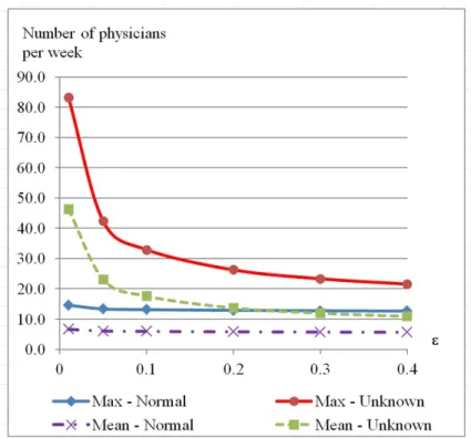
We also compute the performance measurements for only FV patients (Figure 4) or only RV patients (Figure 5). The results show that an increase of the violation risk leads to a decrease in the required capacity for both the maximum and the mean values. Similarly, knowing that the demand comes from a normal distribution reduces the required capacity.
Figure 4: The number of FV full-time equivalent physicians required for the normal and unknown distributions.
Finally, we compare the performance of the deterministic equivalents to the deterministic models in Nguyen et al. (2015). The capacity plan from the deterministic model, however, would result in the risk of violation being greater than 40%. The maximum required capacity from the deterministic model corresponds to 14.2 full-time equivalent physicians per week. To assure the risk of violation to be not greater than 40%, from model (P1-a) we need 15.6 full-time equivalent physicians per week for normal distribution of the arrivals; from model (P1-b), with partial distributional information of arrivals, we require 24.5 full-time equivalent physicians per week. A similar comparison can be done for the mean required capacity. In either case, the
19 required capacity of the deterministic model (14.2 full-time equivalent physicians) is less than that of the approximated models with a risk of violation at 40%; thus, the results from the deterministic model in Nguyen et al. (2015) cannot guarantee the risk of violation to be less than 40%.
Figure 5: The number of RV full-time equivalent physicians required for the normal and unknown distributions
The above analyses provide a conservative and tractable method for capacity planning of the re-entry system. The proposed approximations produce a stable and robust solution for a range of risk levels of patients rejected. In addition, if the arrivals can be assumed to follow a normal distribution, then the required capacity level can be reduced greatly.
4.3. Pattern of scheduling an appointment
We conducted a large numerical experiment with 450 test cases. The 450 test cases are specified from 5 different sets of discharge rates, 6 levels of the RV’s mean lead-time, and 15 different set of appointment lead-time targets. For each of the 450 test cases, we determine the capacity plans for 6 levels of the violation risk = {0.01; 0.05; 0.10; 0.20; 0.30; 0.40}.Thus, (6 × 450) × 2 =
20 5,400 runs were set up and solved for the two deterministic equivalent models. From these results we find that the patients’ appointments should be set to the median, the 95th percentile, or the 100th percentile appointment date. This finding is similar to that in Nguyen et al. (2015). Table 2: Percentage of patients whose lead-time is equal to one of appointment lead-time targets
Arrival
demands Targets appointment lead-time of patients’
Percentage of patients (%)
Min Median Max Mean
Normal distribution Median 21.0 36.5 44.0 34.2 95th percentile 21.0 30.5 33.0 29.0 100th percentile 3.0 5.0 5.0 4.7 Unknown distribution Median 4.0 31.0 46.0 28.9 95th percentile 15.0 21.5 22.0 20.0 100th percentile 3.0 5.0 5.0 4.7
Table 2 reports the percentage of the FV patients whose appointment is set to one of the appointment lead-time targets for the deterministic equivalents. With normally distributed arrivals, an average of 34.2%, 29%, and 4.7% of the FV patients are scheduled at the median, 95th percentile, and 100th percentile appointment lead-time targets, respectively. With limited distributional information of the arrivals, an average of 28.9%, 20%, and 4.7% of the FV patients have their appointments scheduled at the median, 95th percentile, and 100th percentile appointment lead-time targets, respectively. The results show that, for both cases, a majority of the appointments are set at one of the three appointment lead-time targets.
We fit two linear regression models to estimate the relationship between the FV’s mean appointment lead-time, 𝑙̅ and 𝑙̅ , and the appointment lead-time targets, u, v and w, for the numerical results from the test runs. The fitted models in equations (29) and (30) are similar to results in Nguyen et al. (2015).
𝑙̅ = 0.46𝑢 + 0.45𝑣 + 0.05𝑤 + 0.05 (29)
𝑙̅ = 0.42𝑢 + 0.45𝑣 + 0.05𝑤 + 0.02 (30)
The results seem to imply that the deterministic equivalent models can lead to similar FV’s mean appointment lead-times regardless of the assumed arrivals distribution. However, if the arrivals are from a normal distribution, then more patients have an appointment either on the
21 median, on the 95th percentile, or on the 100th percentile appointment date. We did not find any pattern from the scheduling of RV patients. In addition, we found no relation between the discharge rates, lead-time targets, and violation risks to the number appointments that are scheduled on one of the appointment lead-time dates.
4.4. Sensitivity analysis
We now examine the sensitivity of the model’s performance measures to changes to the FV’s appointment lead-time targets, to the violation risk, to the discharge rates, and to the restriction of the RV’s mean appointment lead-time. We present the analysis (Tables 3 and 4) based on 15 settings for the FV’s appointment lead-times, 3 possible values for the violation risk (), 5 different levels for each of the discharge rates, and for the actual RV’s mean appointment lead-time target (which is 16 weeks)..
a. Sensitivity analysis to the changes of the FV’s appointment lead-time
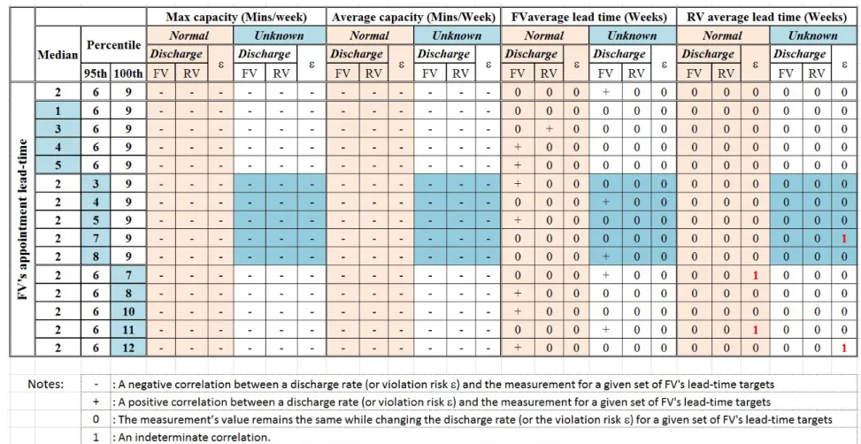
In Table 3, we report the sensitivity of four performance measures to the FV appointment lead-time targets. The four performance measures are the maximum required capacity, the average required capacity, the FV’s mean appointment time, and the RV’s mean appointment lead-time. We report the sensitivity to changes in the median, or the 95th percentile, or the 100th percentile of the appointment lead-time target for three levels of the violation risk () (Table 3).
The results show that the maximum required capacity decreases as the appointment lead-time targets increase. The finding is expected and consistent for all discharge rates. Secondly, the average required capacity is negatively correlated or indeterminate to the changes of the appointment lead-time targets. Thirdly, the FV’s mean appointment lead-time tends to have a positive correlation to the changes of the appointment lead-time targets. This trend may not remain when the discharge rates are high. Finally, the RV’s mean appointment lead-time remains unchanged to the changes of the appointment lead-time targets. The relations between the performance measures and the FV’s appointment lead-time targets are generally consistent across the different levels of violation risk, and the different pairs of the discharge rates, and with either normal or unknown demand distribution.
22 Table 3: Sensitivity analysis to the changes of the FV’s appointment lead-times, with the actual RV’s mean appointment lead-time.
23 Table 4: Sensitivity analysis to the changes of the discharge rates and the change of the violation risk (), with the actual RV’s mean appointment lead-time.
24 b. Sensitivity analysis to the changes of the discharge rates and to the change of the
violation risk (e)
In Table 4, we report the sensitivity of four performance measures to changes of the FV and RV discharge rates, and to changes in the violation risk (). The performance measures are again the maximum required capacity, the average required capacity, the FV’s mean appointment lead-time, and the RV’s mean appointment lead-time. The maximum required capacity and average required capacity decline as the FV discharge rate increases, as the RV discharge rate increases, and as the violation risk increases. This trend is consistent for all examined sets of the appointment lead-time targets. The FV’s mean appointment lead-time either remains the same or increases when a discharge rate increases; however, it seems not to be affected by the violation risk. The RV’s mean appointment lead-time may remain unchanged to the changes of the discharges rates; but it could be indeterminate to the change of the violation risk in some cases. These findings seem consistent for both normal and unknown arrival distributions.
5. Discussion and conclusion
We have developed deterministic equivalent models for determining the maximum required capacity for a re-entry system with uncertain arrivals. The models are formulated so as to satisfy restrictions on the FV patients’ median, 95th percentile, and 100th percentile appointment lead-times, and the satisfaction of the RV patients’ appointment lead-time. The objective of the problem in both models is to minimize the maximum required capacity. Since the arrivals are uncertain, we need to control for the possibility of not having sufficient capacity; we do this by imposing an acceptable risk of violation within the model. We consider two cases, one in which the distribution of arrivals is known and the other when it is not known
The numerical experiments show that allowing a higher risk of violation leads to a lower requirement of planned resource. This pattern is consistent regardless of whether the arrival distribution is known or not. Furthermore, knowing the arrival distribution (e.g. normal distribution) could dramatically reduce the required level of capacity.
Moreover, we find that FV patients’ appointment should generally be scheduled at one of the appointment lead-time targets. This appointment scheduling for FV patients is independent from the information of the FV arrivals distribution and the violation risk. In general, the
25 proposed models are effective at simply relating the appointment lead-time scheduling strategy to a required resource plan based on some specified acceptable level of risk violation.
However, the proposed approximations are limited by the consideration of a single category of patients, for which all patients have the same consultation time, the same FV appointment lead-time targets, the same RV appointment lead-time, the same discharge rates, and be under the same distributional information. Therefore, if the system has a seasonal arrivals pattern, then we would need to extend the models. Furthermore, for different categories of patients, randomness of the discharge rates should also be included to generalize the proposed models. With the success of the mentioned extension, it will enhance the applicability of the proposed approach.
Appendix A: summary the required capacity for different levels of the violation risk
Total required capacity (weekly)
Number of required slots Number of required full-time equivalent physicians
Model Deterministic (Nguyen et al., 2015) Stochastic Deterministic (Nguyen et al., 2015) Stochastic Risk of Violation ( ) - 0.01 0.05 0.1 0.2 0.3 0.4 - 0.01 0.05 0.1 0.2 0.3 0.4 FV & RV Max Normal 683 825 781 771 760 754 749 14.2 17.2 16.3 16.1 15.8 15.7 15.6 Unknown 4077 2171 1719 1399 1259 1175 84.9 45.2 35.8 29.1 26.2 24.5 Mean Normal 521 632 602 595 587 583 580 14.2 17.2 16.3 16.1 15.8 15.7 15.6 Unknown 2870 1560 1248 1028 931 873 84.9 43.1 35.8 29.1 26.2 24.5 FV Max Normal 386 467 427 420 413 408 405 12.1 14.6 13.3 13.1 12.9 12.8 12.7 Unknown 2663 1354 1053 840 746 690 83.2 42.3 32.9 26.3 23.3 21.6 Mean Normal 136 212 194 190 186 183 181 4.3 6.6 6.1 5.9 5.8 5.7 5.7 Unknown 1483 739 562 437 382 349 46.3 23.1 17.6 13.7 11.9 10.9 RV Max Normal 683 825 781 771 760 754 749 14.2 17.2 16.3 16.1 15.8 15.7 15.6 Unknown 4077 2171 1719 1399 1259 1175 84.9 45.2 35.8 29.1 26.2 24.5 Mean Normal 385 421 408 405 402 400 398 8 8.8 8.5 8.4 8.4 8.3 8.3 Unknown 1387 821 686 591 549 525 28.9 17.1 14.3 12.3 11.4 10.9
26 Appendix B: Proof of the constraints (29):
The proof is done for every individual constraint in the set of constraints (25). Given constraint i of the set of constraints (25), the constraint 𝑃𝑟 𝑓 − ∑ 𝑧 ≤ 0 ≥ 1 − is equivalent to:
𝑃𝑟 𝑓 − ∑ 𝑧 > 0 ≤ (31)
The left hand side of the constraint can be written as:
𝑃𝑟 𝑓 − ∑ 𝑧 > 0 = 𝑃𝑟 𝑓 > ∑ 𝑧 = 𝑃𝑟 >∑ (32)
Then, we obtain:
𝑃𝑟 𝑓 − ∑ 𝑧 > 0 ≤ 𝑃𝑟 >∑ ≤ 𝑃𝑟 ≥ ∑ (33)
We use Chebyshev’s inequality (Savage, 1961), i.e., 𝑃𝑟(|𝑋 − 𝜇| ≥ 𝑘𝜎) ≤ , to write: 𝑃𝑟 𝑓 − ∑ 𝑧 > 0 ≤
∑ (34)
Thus the original constraint (30) is guaranteed if:
∑ ≤ (35)
The above constraint (35) can be transformed into a linear constraint as in the constraint (28).
Acknowledgement:
The authors would like to thank Singapore – MIT Alliance programme for funding this doctoral research. The authors are grateful Tan Tock Seng Hospital, Singapore for providing us the opportunity to study this interesting field. The authors would like to thank Dr. Jamie Mervyn Lim and the hospital’s administrators for providing data and necessary help to conduct this research. The authors cannot forget to thank the anonymous reviewers for constructive and valuable comments which greatly improve the manuscript.
27 References
1. Ahmadi-Javid, A., Jalali, Z., and Klassend, K.J. (2016). Invited review. Outpatient appointment systems in healthcare: a review of optimization studies. European Journal of Operational Research, 1-32.
2. Balasubramanian, H., Biehl, S., Dai, L., and Muriel, A. (2014). Dynamic allocation of same-day requests in multi-physician primary care practices in the presence of prescheduled appointments. Health Care Management Science 17, 31-48.
3. Bamford, D. andChatziaslan, E. (2009). Healthcare capacity measurement. International Journal of Productivity and Performance Management 58(8), 748-766.
4. Bennett, J.C. and Worthington, D.J. (1998). An example of a good but partially successful OR engagement: improving outpatient clinic operations. Interface 28(5), 56-69.
5. Bertsimas, D. and Tsitsiklis, J.N. (1997). Introduction to Linear Optimization, page: 272-278. Athena Scientific, Belmont, Massachusetts, USA.
6. Bowers, J., Lyons, B., Mould, G., Symonds, T. (2005). Modelling outpatient capacity for a diagnosis and treatment centre. Health Care Management Science 8(3), 205-211.
7. Bowers, J. (2010). Waiting list behavior and the consequences for NHS targets. Journal of the Operational Research Society 61(2), 246-254.
8. Calafiore, G.C. and Ghaoui, L.E. (2006). On distributionally robust chance-constrained linear programs. Journal of Optimization Theory and Applications 130(1), 1-22.
9. Cayirli T., and Veral E. (2003). Outpatient scheduling in healthcare: A review of literature. Production and Operations Management 12 (4), 519 -549.
10. Cayirli, T., Gunes, E.D. (2014). Outpatient appointment scheduling in presence of seasonal walk-ins. Journal of the Operational Research Society 65, 512-531.
11. Charnes, A. and Cooper, W.W. (1963). Deterministic equivalents for optimizing and satisficing under chance constraints. Operations Research 11(1), 18-39.
12. Creemers, S., Belien, J., and Lambrecht, M. (2012). The optimal allocation of server time slots over different classes of patients. European Journal of Operational Research 219, 508-521. 13. Demir, E., Chahed,S., Chaussalet, T., Toffa, S., and Fouladinajed, F. (2012). A decision support
tool for health service re-design. Journal of Medical Systems 36(2), 621-630.
14. Elkhuizen, S.G., Das,S.F., Bakker, P.J.M., and Hontelez, J.A.M. (2007). Using computer simulation to reduce access time for outpatient departments. Quality and Safety in Health Care 16(5), 382-386.
28
15. Green, L.V, Savin, S., and Wang, B. (2006). Managing patient service in a diagnostic medical facility. Operations Research 54(1), 11-25.
16. Green, L.V.,Savin, S. (2008).Reducing delays for medical appointments: A queueing approach. Operations Research 56(6), 1526-1538.
17. Ittig, P.T. (1985). Capacity planning in service operations: The case of hospital outpatient facilities. Socio-Economic Planning Sciences 19(6), 425-429.
18. Kemper B., Klaassen C.A.J, Mandjes M. (2014). Innovative application of OR. Optimized appointment scheduling. European Journal of Operational Research 239, 243-255.
19. Kuiper, A., and Mandjes M. (2015). Appointment Scheduling in tandem-type service systems. Omega 57, 145-156.
20. Leitch, A.G., Parker, S., Currie, A., King, T., and McHardy, G.J.R (1990). Evaluation of the need for follow-up in an out-patient clinic. Respiratory Medicine 84(2), 119-122.
21. LaGanga, L.R, and Lawrence, S.R. (2012). Appointment overbooking in health care clinics to improve patient service and clinic performance. Production and Operations Management 21(5), 874-888.
22. Liu, N. (2016). Optimal choice for appointment scheduling window under patient no-show behavior. Production and Operations Management 25(1), 128-142.
23. Mak, H.Y, Rong, Y., and Zhang, J. (2016). Appointment scheduling with limited distributional information. Management Science 61(2), 316-334.
24. Nemirovski, A. and Shapiro, A. (2006). Convex approximations of chance constrained programs. Society for Industrial and Applied Mathematics on Optimization 17(4), 969-996.
25. Nguyen, T.B.T., Sivakumar, A.I., and Graves, S.C (2015). A network flow approach for tactical resource planning in outpatient clinics. Health Care Management Science, 18 (2), 124-136.
26. Nguyen, T.B.T., Sivakumar, A.I., and Graves, S.C (2016). Scheduling rules to achieve lead-time targets in outpatient appointment systems. Health Care Management Science, DOI: 10.1007/s10729-016-9374-2.
27. Ozcan Y.A. (2005). Quantitative methods in health care management: techniques and applications. Jossey-Bass, A Wiley Imprint, USA.
28. Patrick, J. Puterman, M.L., Queyranne, M. (2016). Dynamic multipriority patient scheduling for a diagnostic resource. Operations Research 56(6), 1507-1525.
29. Porta-Sales, J., Codorniu, N., Gomez-Batiste, X., Alburquerque, E., Serrano-Bernudez, G., Sanchez-Posada, D., Perez-Martin, X., Gonzalez-Barboteo, J., and Tuca-Rodriguez, A. (2005). Original article: Patient appointment process, symptom control and prediction of follow-up
29
compliance in a palliative care outpatient clinic. Journal of Pain and Symptom Management 30(2), 145-153.
30. Qu, S., Rardin, R.L., Williams, J.A.S., Willis, D.R. (2007). Matching daily healthcare provider capacity to demand in advanced access scheduling systems. European Journal of Operational Research 183(2), 812-826.
31. Qu, X. and Shi, J. (2009). Effect of two-level provider capacities on the performance of open access clinics. Health Care Management Science 12(1), 99-114.
32. Qu, X., Rardin, R.L., Williams, J.A.S. (2011). Single versus hybrid time horizons for open access scheduling. Computers & Industrial Engineering 60(1), 56-65.
33. Qu, S. Rardin, R.L., and Williams, J.A.S. (2012). A mean-variance model to optimize the fixed versus open appointment percentages in open access scheduling systems. Decision Support Systems 53, 554-564.
34. Qu, X., Peng, Y., Kong, N., and Shi, J. (2013). A two-phase approach to scheduling multi-category outpatient appointments- A case study of a women’s clinic. Health Care Management Science 16, 197-216.
35. Ross, S. M. (1993). Introduction to Probability Models, fifth edition, page: 1-20. Academic Press limited, UK.
36. Saure, A., Patrick, J., Tyldesley, S., Puterman, M.L. (2012). Innovative applications of O.R. Dynamic multi-appointment patient scheduling for radiation therapy. European Journal of Operational Research 223, 573 -584.
37. Savage, R. (1961). Probability inequalities of the Tchebycheff type. Journal of Research of the National Bureau of Standards – B. Mathematics and Mathematical Physic 65B (3).
38. Street, A. and Duckett, S. (1996). Are waiting lists inevitable? Health Policy 36(1), 1-15.
39. Thomas, S.J., Williams, M.V., Burnet, N.G., and Baker, C.R. (2001). How much surplus capacity is required to maintain low waiting time? Clinical Oncology 13(1), 24-28.
40. Worthington, D. (1991). Hospital waiting list management models. The Journal of the Operational Research Society 42(10), 833-843.