Publisher’s version / Version de l'éditeur: PERD/CHC Report, 9-77, 1998-05
READ THESE TERMS AND CONDITIONS CAREFULLY BEFORE USING THIS WEBSITE. https://nrc-publications.canada.ca/eng/copyright
Vous avez des questions? Nous pouvons vous aider. Pour communiquer directement avec un auteur, consultez la première page de la revue dans laquelle son article a été publié afin de trouver ses coordonnées. Si vous n’arrivez pas à les repérer, communiquez avec nous à [email protected].
Questions? Contact the NRC Publications Archive team at
[email protected]. If you wish to email the authors directly, please see the first page of the publication for their contact information.
Archives des publications du CNRC
For the publisher’s version, please access the DOI link below./ Pour consulter la version de l’éditeur, utilisez le lien DOI ci-dessous.
https://doi.org/10.4224/12340999
Access and use of this website and the material on it are subject to the Terms and Conditions set forth at
A lattice model of ice failure
Sayed, M.; Timco, G. W.
https://publications-cnrc.canada.ca/fra/droits
L’accès à ce site Web et l’utilisation de son contenu sont assujettis aux conditions présentées dans le site LISEZ CES CONDITIONS ATTENTIVEMENT AVANT D’UTILISER CE SITE WEB.
NRC Publications Record / Notice d'Archives des publications de CNRC: https://nrc-publications.canada.ca/eng/view/object/?id=16af6486-3ac6-4036-9702-bcc3d13c0677 https://publications-cnrc.canada.ca/fra/voir/objet/?id=16af6486-3ac6-4036-9702-bcc3d13c0677
M. Sayed and G.W. Timco Canadian Hydraulics Centre National Research Council of Canada
Ottawa, Ont. K1A 0R6 Canada
Technical Report HYD-TR-035 PERD/CHC Report 9-77
ABSTRACT
A numerical model of the failure of ice features against structures is developed. The formulation is based on discretizing the ice mass to a set of nodes that are linked by breakable elements. The contact elements consist of arrangements of springs and dashpots, which represent the required rheology (e.g elastic or visco-elastic behaviour). Fracture is introduced according to a macro failure criterion (e.g. tensile strength). A set of equations describing the momentum balance of the nodes is solved to give the velocities and displacements at each time step.
The model is applied to cases of uni-axial compression, plane indentation, and ridge impact on structures. Both brittle and visco-elastic behaviours are examined. The simulations predict stresses, initiation and propagation of cracks, as well as velocity and displacement fields. The resulting stresses are found to agree with available data.
TABLE OF CONTENTS
ABSTRACT ... i
TABLE OF CONTENTS ...ii
LIST OF FIGURES...iii
1 INTRODUCTION... 1
2 LATTICE MODEL ... 3
2.1 Overview ... 3
2.2 Simulation Procedures... 3
2.3 Rheology of the Contact Elements... 5
2.3.1 Brittle model... 5 2.3.2 Visco-elastic model ... 6 3 UNIAXIAL COMPRESSION ... 7 3.1 Brittle model... 7 3.2 Visco-elastic deformation ... 8 4 INDENTATION... 11 4.1 Brittle Failure ... 11 4.2 Visco-elastic deformation ... 17
5 RIDGE IMPACT AGAINST STRUCTURES ... 19
6 SUMMARY AND CONCLUSIONS... 26
7 ACKNOWLEDGEMENTS ... 27
8 REFERENCES... 27
PERD Documentation Page NRC Documentation Page
LIST OF FIGURES
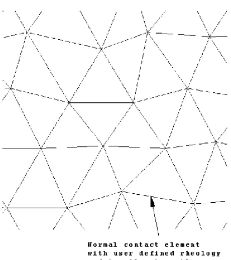
Figure 1 A portion of 60 x 50 lattice used in the simulations. With this lattice model, individual elements will break if the tensile stress exceeds the tensile strength
of the element. ... 4
Figure 2 Rheological model representing brittle behaviour... 6
Figure 3 Rheological model representing visco-elastic behaviour. ... 6
Figure 4 Boundary conditions for uniaxial loading. ... 7
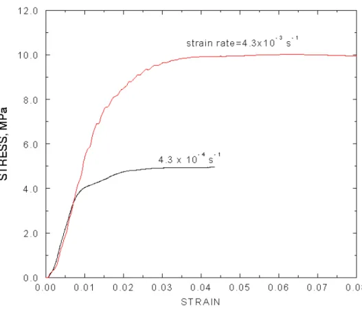
Figure 5 Stress-strain plots showing visco-elastic yield for two strain rates. ... 9
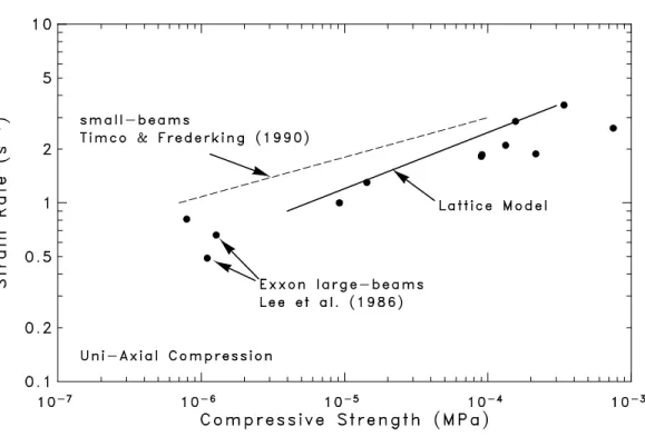
Figure 6 Compressive strength of sea ice as predicted by the model. Values of measured small-scale and large-scale experiments are included for comparison. ... 10
Figure 7 Boundary conditions for plane indentation runs... 11
Figure 8 Sequence of images showing the evolution of the stress distribution and cracking pattern during indentation. ... 15
Figure 9 Average stress on the indentor versus displacement for brittle failure and various tensile strengths. ... 16
Figure 10 Total crack length per unit area versus displacement for brittle failure and various tensile strengths. ... 16
Figure 11 Average stress on the indentor versus displacement for various strain rates using the visco-elastic model. ... 17
Figure 12 Maximum stress versus strain rate for the indentation tests with the visco-elastic elements. The figure shows results for two different tensile strengths, representing freshwater ice and sea ice. ... 18
Figure 13 Total crack length per unit area versus displacement for various strain rates using the visco-elastic model. ... 18
Figure 14 Geometry of the ridge and structure, Ridge 1... 19
Figure 15 Horizontal force on the structure versus time, Ridge 1. ... 20
Figure 16 Vertical force on the structure versus time, Ridge 1... 21
Figure 17 Distribution of normal contact pressures after 0.1 s, 0.2 s and 1 s from the start of the interaction, Ridge 1. ... 22
Figure 18 Geometry of ridge with rigid top boundary, Ridge 2. ... 23
Figure 19 Horizontal force on the structure versus time, Ridge 2. ... 24
A Lattice Model of Ice Failure
1 INTRODUCTION
Failure of floating ice features against structures and ships usually involves the propagation of multiple large cracks, fragmentation, and rubble accumulation. Such situations have so far been beyond the capabilities of numerical and analytical solutions. Although the available approaches can be useful in some instances, they cannot follow the complex interaction and the failure of the ice, particularly its disintegration and flow. Finite element solutions, for example, have been successfully applied to deal with a few idealized situations (e.g. Morsey and Brown, 1993). In such cases, the models can fit particular data sets by using several arbitrary parameters. Those models, however, cannot predict a priori the loads on a structure. These models cannot take into account all of the complexities of the interaction process. In many situations, failure processes are governed by propagation of cracks of lengths comparable to dimensions of the ice feature (Blanchet, 1990); however, existing numerical models cannot realistically simulate this failure mode. This limits the applicability of the solutions. Continuum damage models have been used to describe the intensity of small cracks (e.g. Wu and Shyam-Sunder, 1991) but they also cannot deal with large cracks propagation and interaction.
More recently, discrete element models have been introduced in ice forecasting and in the study of ice jams. The earliest such study was carried out by Shen et al. (1987) to model a marginal ice zone. Other related work include an examination of meso-scale yield conditions by Hopkins (1993), and an examination of broken ice interaction with offshore structures by Loset (1994). Yamaguchi et al. (1993) used a discrete element formulation to model ice flow in channels. Another discrete model for meso-scale ice forecasting was developed by Savage (1995). That formulation was further extended by Sayed et al. (1995) to examine yield conditions of broken and intact ice covers.
Lattice-based numerical models have been developed to simulate the behaviour of inhomogeneous materials. Unlike discrete models, which only account for compressive normal forces at the contact between particles, lattice models introduce tensile forces at the contacts. The approach is based on discretizing the material into a set of nodes. Each node can interact with a limited number of neighbours through contact elements that are allowed to break. This approach is suited for including inhomogeneity of the material and simulating the propagation of multiple cracks. Another advantage of this approach is that only simple models of material behaviour and strength need to be used for the contact elements. Starting with simple and physically plausible assumptions, the simulations can produce very complex modes of failure. Reviews of lattice models were given by Herrmann and Roux (1990), and Roux (1990). Applications of lattice models include studies of fracture of cement-based composites by Schlangen and van Mier (1992), and fracture of brittle materials by Dai and Frantziskonis (1994). The tensile forces and fracture were introduced by Sayed et al. (1995) in order to model the behaviour of intact
ice cover. An overview of applications of lattice models to floating ice problems was also given by Sayed (1997).
The emphasis of this report is on presenting model formulation and simulation approach of a lattice model applied to brittle and visco-elastic deformation of ice. As illustrations of applicability, the model is applied to cases of uniaxial compression, failure of an ice sheet against a flat indentor, and ridge impact against structures. Model predictions are compared to available experimental data for those cases. Although the presentation in this report describes two-dimensional deformation, three-dimensional simulations can be done with only minor changes.
2 LATTICE MODEL
2.1 Overview
The ice mass is represented by a set of nodes in a lattice. Each node is connected to its immediate neighbours by contact elements, which consist of springs and dashpots. The contact elements model the relationship between the forces and relative displacements and velocities of the nodes. Normal, tangential and torsional elements can be used. Various rheologies can be introduced by choosing the appropriate arrangements and constants for the springs and dashpots. Crack formations are simulated by allowing the contact elements to break. When the force in a contact element exceeds its strength, the link is broken. Broken normal elements can only transmit compressive forces.
Movements of the nodes are governed by the momentum balance equations. Boundary conditions may consist of applied displacements, displacement rates or forces. Body forces (e.g. gravity) can be applied to the nodes as well. As fragments form and drift, nodes may come in contact with new nodes other than the original neighbours. Simulations can be carried out to track new contacts, and the interaction between fragments.
2.2 Simulation Procedures
In this report, two-dimensional deformation is considered. Nodes are placed in a plane to form irregular triangles such that each node is linked to six neighbours (see Fig. 1). The lattice is constructed by starting with equilateral triangles of side length l. The nodes are next given random displacements of ±0.15 l along the horizontal and vertical directions. Preliminary runs showed that a lattice of uniform equilateral triangles could influence the directions of crack propagation. In that case, cracks may tend to propagate along directions parallel to triangle sides. Therefore, randomness was incorporated in the lattice to prevent crack propagation along preferred directions.
The simplest form of contact elements, which are normal elements, are used. There is no evidence at present to indicate that tangential and rotational elements are needed. Movements of the nodes are governed by the equations of linear momentum. Since shear and torsional contact elements are not used, the angular momentum equations are not needed. The balance of linear momentum for each node may be expressed as
m du
dt = i=1 F
N i
where m is the mass assigned to the node, u is the velocity vector, t is time, and i=1 N
i
F
Σ is
the vector sum of contact forces due to N contacts. Body forces are not needed in the following examples, but they can be easily included in Eq. 1.
Figure 1 A portion of 60 x 50 lattice used in the simulations. With this lattice model, individual elements will break if the tensile stress exceeds the tensile strength of the element.
The initial conditions consist of prescribed positions and velocities for all nodes. Boundary conditions usually consist of fixed velocities or positions for certain nodes. At the beginning of a simulation, a list of contacts for each node is determined. The list includes neighbouring node identification numbers, contact element lengths, and whether the contacts are intact or broken. In the following examples, all contacts are considered intact at the start of the simulation. The time step loop is then started. At each time step, positions and velocities of the nodes are updated by numerically integrating the velocities and accelerations. Contact forces are next determined by solving a set of momentum equations (Eq. 1). Each contact element is tested for breaking condition. Forces are then adjusted accordingly, and the list of broken contacts updated.
In order to simulate the behaviour of fragmented ice, the list of contacts has to be periodically updated. The list should include nodes in the “neighbourhood” of each node. The frequency of updating that list and the area identified as a “neighbourhood” depend on the particular problem under study. When calculating distances between nodes of drifting fragments, each node is considered to be at the centre of a disk of radius l/2. Note that original contacts in the lattice have variable lengths. Keeping track of fragmented ice follows standard molecular dynamics simulations (e.g. Allen and Tildsley, 1987). The time step has to be kept relatively small. Also a Verlet algorithm is used in order to improve the accuracy of velocity and position calculations.
2.3 Rheology of the Contact Elements
As discussed above, various rheological models can be used for the contact elements between the nodes. They can be as simple or as complex as required for addressing any particular problem. As an illustrative example, two different simple models are used in this paper. They are intended to demonstrate the flexibility of the lattice model for ice failure problems. For one, a simple linear-elastic, brittle model is used. For the second, the visco-elastic behaviour of ice is modelled.
2.3.1 Brittle model
The normal forces between the nodes are calculated using linear springs and dashpots as shown in Fig. 2. The force, Fn between two nodes is the sum of the forces in the spring
and the dashpot, and may be expressed as follows
where k is the spring constant, b is the dashpot constant, δ is the relative normal displacement (change in the length of the element), and vn is the relative normal velocity.
This type of contact element represents elastic behaviour, with all deformation fully recoverable. The dashpot is included here to account for the viscous damping needed for energy dissipation. If the normal force exceeds the tensile strength St of the contact
element, the element breaks. No tensile forces are allowed at that contact afterwards. Thus, the above model represents brittle failure. Inhomogeneities can be easily introduced by assigning variable stiffness (or spring constants) and strengths to the contact elements.
n n k v
Figure 2 Rheological model representing brittle behaviour.
2.3.2 Visco-elastic model
There is a large body of literature that deals with the visco-elastic behaviour of small ice samples (e.g. Sinha, 1978 and 1991; Sjölind, 1987; Duval et al., 1991). For the present approach, only the simplest aspects of that behaviour are included which can produce rate effects and irreversible deformation. A schematic of a simple visco-elastic contact model is shown in Fig. 3. The spring is considered to be linear but the dashpot is chosen to represent nonlinear creep according to Glen’s law. The force between two nodes, Fn
would be equal to the force in the spring and the force in the dashpot as follows
where B is a constant for the nonlinear dashpot. The present model corresponds to the simplest choice that gives the required visco-elastic behaviour. The model accounts for secondary creep, but not other aspects of deformation such as primary and tertiary creep. Thus the model gives an upper limit for the stresses. The visco-elastic case requires additional steps for calculating contact forces. The relative displacement at each contact has to be divided into an elastic part and a viscous irreversible part. That involves solving the cubic equation, which equates the elastic force of the spring to the viscous force of the dashpot.
Figure 3 Rheological model representing visco-elastic behaviour.
n n
1/3
3 UNIAXIAL COMPRESSION
3.1 Brittle model
A test case of uniform axial compression (Fig. 4) was first done in order to calculate Poisson’s ratio, and to determine the relationship between the continuum stress (or strength) and forces (or strengths) of the contact elements. The test also determines the relationship between the continuum elastic modulus and spring constants of the contact elements. A 60 x 50 node lattice was used in the simulations.
Boundary conditions were implemented by applying uniform downward displacement at a constant velocity to the top boundary. Nodes along the bottom boundary were fixed along the y-direction, but were allowed to move freely in the horizontal direction.
Figure 4 Boundary conditions for uniaxial loading.
For the brittle case, described by Eq. 2, the following simulation parameter values were used: a strain rate of 0.0224 s-1, a time step of 1.78 x 10⁻⁴ s, and a maximum strain of 0.025. The lattice was held at that displacement to allow stresses and strains to reach steady values. Values of the viscous dashpot constant between 0.1 and 2.0 were used. Changing the viscous damping within that range had negligible influence on the resulting stress rate. The higher values of that constant dampened the stress fluctuations slightly faster. No fracture was allowed to take place in these tests.
The resulting Poisson ratio was 0.33, which is a reasonable value for elastic behaviour. This value is also in agreement with that determined by Dai and Frantziskonis (1994).
The lattice model deals with forces and strengths of contact elements. It is desirable to relate the forces and stiffnesses of the contact elements to the corresponding continuum parameters that are known from laboratory experiments. The continuum stress σ was found to depend on the average contact force, Fn and average distance between nodes, l as
follows:
where h is the thickness of the test sample. The relationship between the continuum tensile strength and strength of individual contact elements should be similar to Eq. 4.
3.2 Visco-elastic deformation
Uniaxial compression tests were done to examine visco-elastic yield behaviour. No fracture was allowed in this case in order to avoid splitting of the unconfined samples, which would obscure the visco-elastic deformation behaviour. A value of the nonlinear dashpot constant, B = 19 MN s1/3 / m1/3 appeared to give a reasonable relationship between peak stress and strain rate.
The resulting stress-strain relationship is illustrated in Fig. 5, which shows how stresses increase with increasing strain until the maximum yield stress is reached. A line representing the dependence of yield stress on strain rate behaviour is plotted in Fig. 6. The figure also includes the results of small sea ice beam tests (Timco and Frederking, 1990), and the large (6 x 3 x 1.5 m) sea ice beams tested in compression by Exxon (Lee et al., 1986). There is good agreement between the values calculated by the lattice model with the experimentally measured compressive strength for sea ice.
Figure 6 Compressive strength of sea ice as predicted by the model. Values of measured small-scale and large-scale experiments are included for comparison.
4 INDENTATION
4.1 Brittle Failure
The boundary conditions shown in Fig. 7 were used to study the indentation. The following parameter values were used for the case of brittle failure:
distance between nodes l = 1 m thickness h = 1 m spring constant k = 109 N/m dashpot constant b = 28 kN s/m specific gravity = 0.91 velocity = 0.11 m/s time step = 1.78 x 10⁻⁴ s
Figure 7 Boundary conditions for plane indentation runs.
The ice cover consisted of 50 x 60 nodes, which corresponds to a 50 m x 60 m rectangle. Testing a range of velocities showed that the value of 0.11 m/s was sufficiently small to avoid any detectable inertial effects; i.e stresses arose only due to failure of the lattice.
The above value of the spring constant corresponds to a lower elastic modulus than the values measured for small ice samples. At the larger scales relevant to the present example, imperfections in the ice cover would decrease the elastic modulus. In addition, using a higher spring constant would have required using smaller time steps. It should be noted that lattice stiffness affects indentation displacements, but not the stresses. The effect of node spacing, l was examined by testing several indentor widths, w. Simulations were done using indentor widths of 4 m, 5 m and 10 m (corresponding to w/l = 4, 5 and 10), and a tensile strength of 0.4 MPa. Stresses were relatively high for w/l of 4, then became constant with increasing w/l. Thus it appears that a value of w/l = 4 is adequate to eliminate any artifacts of the lattice.
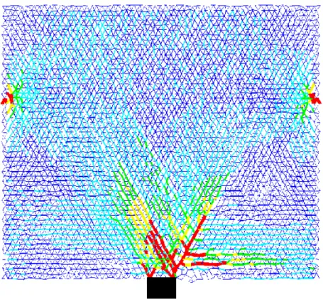
An example of the evolution of the stress distribution and fracture patterns is shown in a sequence in Fig. 8. In this case, a 6 m wide indentor interacts with ice which has a tensile strength of 0.4 MPa. Cracks start to propagate from the corners of the indentor, where stresses are the highest. After that, several long cracks propagate in front of the indentor. Note that a few cracks occur at the boundaries, where constant velocity is applied to the ice sheet. It is difficult to quantify the experimental observations of crack patterns, but available observations (e.g. Timco, 1987) appear in general agreement with the present results.
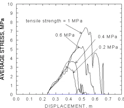
These plots demonstrate the fracture process for the situation of an ice sheet with a tensile strength of 0.4 MPa. This would represent relatively weak sea ice. Fig. 9 shows a plot of the mean stresses on the 6 m wide indentor versus displacement for various tensile strengths from 0.2 to 1.0 MPa. The lower range of tensile strengths are indicative of the range for sea ice (Richter-Menge and Claffey, 1991), whereas the upper value of 1.0 MPa would be representative of freshwater ice (Gold, 1977). As intuitively expected, Fig. 9 shows a strong dependence for failure pressure on the tensile strength of ice.
The resulting crack lengths are shown in Fig. 10. The total length of the cracks in each case is divided by the area of the lattice. As expected, increasing the tensile strength increases the stress and decreases the length of cracks.
The question that follows is “How do these calculated pressures compare with pressures measured during large-scale indentation tests?”. Two data sets can be used for comparison - one for sea ice and the other for freshwater ice. Croasdale (1970) reported on large-scale “nutcracker” tests performed on sea ice. Measured failure pressures ranged from 3.0 to 6.1 MPa. These values are in good agreement with the predicted values of 3.5 to 5.0 MPa for sea ice (Fig. 9). Miller et al. (1974) reported on large-scale indentation in freshwater ice. Failure pressures in the range of 5.4 to 9 MPa were measured for flat indentors of 1.2 m width in ice of thickness 0.6 m. This range of pressures is in excellent agreement with the predicted value of 7.5 MPa for ice with a tensile strength representative of freshwater ice.
Figure 8 Sequence of images showing the evolution of the stress distribution and cracking pattern during indentation.
The present simulations deal with in-plane failure. Moreover, the ice sheet is considered to have uniform stiffness and strength. Under field conditions, ice failure against a flat indentor may include three-dimensional deformation (e.g. flexural failure and spalling). Also ice may contain inhomogeneities, which would give rise to non-simultaneous failure. These factors often result in an aspect ratio (or size) effect. The present simulations can easily be extended to deal with those aspects; namely three-dimensional and non-simultaneous failure.
Figure 9 Average stress on the indentor versus displacement for brittle failure and various tensile strengths.
Figure 10 Total crack length per unit area versus displacement for brittle failure and various tensile strengths.
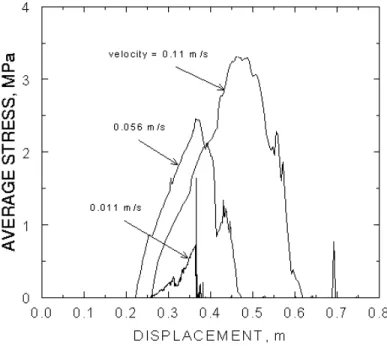
Simulation runs were done using boundary and initial conditions similar to those used above for brittle indentation. Velocities of 0.11 m/s, 0.056 m/s and 0.011 m/s were used in order to examine strain rate effects. An indentor width of 6 m was used in those simulations. Traditionally, a nominal indentation strain rate is estimated as v/(4 w), where v is the velocity. Thus, the above velocities would correspond to nominal strain rates of 4.6 x 10⁻³ s-1, 2.3 x 10⁻³ s-1 , and 4.6 x 10⁻⁴ s-1. These are relatively high strain rates, in the range where fracture failure would predominate over creep behaviour. At these rates, the ice will fracture with rate dependent behaviour. The strain rate effect arises due to the inclusion of a visco-elastic contact element. In this case, large cracks will propagate and interact with one another.
The resulting average stresses on the indentor are plotted versus displacement in Fig. 11 for the three different strain rates. In this case, the lattice elements had a tensile strength of 0.4 MPa, representative of sea ice. There is a definite trend of higher maximum stress with higher strain rates. Similar runs were performed with a lattice with a higher tensile strength of 1 MPa, which would be representative of freshwater ice. Fig. 12 shows a comparison between the maximum stress and strain rate for both types of ice. The plots show higher values for freshwater ice at comparable strain rates, as expected. Crack lengths per unit area are plotted versus displacement in Fig. 13 for the runs with the lower tensile strength. The results show that an increase in strain rate reduces crack lengths. Timco (1987), and Sodhi and Chin (1995) observed this trend in indentation experiments.
Figure 11 Average stress on the indentor versus displacement for various strain rates using the visco-elastic model.
Figure 12 Maximum stress versus strain rate for the indentation tests with the visco-elastic elements. The figure shows results for two different tensile strengths, representing freshwater ice and sea ice.
Figure 13 Total crack length per unit area versus displacement for various strain rates using the visco-elastic model.
5 RIDGE IMPACT AGAINST STRUCTURES
The model was used to examine the modes of failure and forces, which arise when a ridge impacts a structure. Two scenarios were considered. The first scenario consists of a trapezoidal ridge impacting a vertical pier with a conical section near water line. The ridge has a 1 m thick consolidated layer. Both the consolidated layer and sail have a relatively high stiffness and tensile strength, compared to the underwater keel. Geometry of the ridge and the boundary conditions are shown in Fig. 14. The simulations start with the entire ridge moving towards the structure at the initial velocity. The nodes located at the far edge of the ridge opposite the structure (Fig. 14) continue to move at a constant velocity throughout the simulation. This condition represents the movement of pack ice, which drives the ridge against the structure at constant velocity.
Figure 14 Geometry of the ridge and structure, Ridge 1.
The values of simulation parameters are:
node spacing 0.5 ± 0.1 m
velocity 0.2 m/s
spring constant (keel) 1.0 MN/m spring constant (consolidated layer) 10.0 MN/m
dashpot parameter 3.2 kN s/m friction coefficient (ice-ice) 0.3
friction coefficient (ice-structure) 0 ice specific gravity 0.9 tensile strength (keel) 5 kPa tensile strength (consolidated layer) 400 kPa time step 2.14x10⁻⁴ s
The resulting horizontal and vertical forces on the structure are shown in Figs. 15 and 16, respectively. The maximum horizontal force is 0.36 MN/m. The evolution of pressures within the ridge and deformation patterns is illustrated by plotting snapshots of normal contact forces at several intervals as shown in Fig. 17. The highest normal force between nodes in those plots is approximately 100 kPa. The sequence of pressure distributions in Fig. 17 shows the propagation of a pressure wave inside the ridge. The plot corresponding to 1 s after the start of the impact indicates that the consolidated layer is broken. The forces drop at that stage, apparently due to the relief of confinement that was provided by the consolidated layer.
Figure 17 Distribution of normal contact pressures after 0.1 s, 0.2 s and 1 s from the start of the interaction, Ridge 1.
as shown in Fig. 18. In that case, the consolidated layer was replaced with a rigid boundary in order to maximize the confinement of the ridge keel. Geometry of the problem corresponds to a triangular ridge impacting a vertical structure (without a cone). Similarly to the initial conditions of the preceding case, the ridge is assigned a constant velocity at impact. The top horizontal boundary, which replaces the consolidated layer, continues to apply a constant horizontal velocity towards the structure during the simulation.
Figure 18 Geometry of ridge with rigid top boundary, Ridge 2.
The value of simulation parameters remained similar to those used above (except that the sail and consolidated layer were not included). The resulting horizontal force on the structure is plotted versus time in Fig. 19. The maximum forces in the pier are close to those obtained in the preceding case. The increase in confinement apparently had a minor influence on failure of the keel. The resulting pressure distributions after 0.5 s and 1.5 s from the start of the impact are shown in Fig. 20. Those plots show that the pressure distribution, in the absence of a structure’s consolidated layer, is more uniform with higher values close to the water line. As the interaction progresses, it is also evident that part of the keel starts to fracture and separate from the top boundary, which represents the consolidated layer.
The preceding simulations of ridge impact against structures serve to illustrate the manner in which that problem can be analyzed, and provide a few typical results. Obviously, a comprehensive treatment of this problem is beyond the scope of this report. Such a treatment would require an examination of the role of model parameters, geometry, material properties, and boundary conditions, as well as the use of three-dimensional simulations.
Figure 19 Horizontal force on the structure versus time, Ridge 2.
Comparison to field data is not straightforward for these cases. However, comparisons can be made to first-year ridge loads on the offshore structure Molikpaq. This structure, which is 90 m at the waterline, was used for exploratory drilling in the Canadian Beaufort Sea. Typical loads from first-year ridge interaction ranged from 30 to 100 MN. These loads, averaged across the 90 m width give line loads of 0.3 to 1.1 MN/m. This compares reasonably well to the peak loads on the order of 0.4 MN/m calculated using the lattice model. A more detailed verification would be useful, especially if the structure geometry and ridge shape were modelled in a 3-D formulation.
6 SUMMARY AND CONCLUSIONS
A numerical approach has been developed for modelling ice failure and the interaction of ice with structures. The approach is based on discretizing ice covers into nodes that are linked by breakable contact elements. The nodes are placed in a lattice of irregular triangles. The numerical simulations can track the propagation and interaction of multiple large cracks. An additional advantage of this approach is that only a few well-known parameters concerning ice rheology are needed. These parameters describe the stiffness and tensile strength of ice samples. Starting with those well-defined parameters, the simulations can account for the very complex modes of deformation that arise during ice cover failure.
A contact model representing elastic deformation-brittle failure was first examined. Fracture was introduced by assigning a tensile strength to the contact elements, which is related to the continuum tensile strength. The simulations accounted for the initiation and evolution of crack networks. Visco-elastic behaviour was next incorporated in the simulation by including irrecoverable, rate dependent deformation. The contact elements were considered to undergo secondary creep according to Glen’s law.
The model was used to simulate uniaxial compression. The resulting strength-strain rate relationship was in good agreement with available data. The model was next applied to the case of plane indentation. Time records of stresses on the indentor and crack lengths were determined. The results were found to be in agreement with laboratory and field data. Finally, the problem of ridge impact against structures was considered. The simulation results predict forces on the structure, the evolution of pressure distribution within the ridge, and deformation patterns.
The preceding results have proved the feasibility of using lattice models for simulating ice failure against structures. Lattice sizes, which are needed for practical applications (with node numbers of a few tens of thousands) can be adequately handled by available computer speeds, and memory sizes. Extending the present simulations to three-dimensional cases is straightforward. This approach can be used to examine several problems of practical interest, which have so far been beyond the capability of numerical models.
Examples of such problems include:
• the impact of a large floe on a structure, where splitting becomes the critical factor which limits ice force;
• ice rubble pile-up, and its interaction with impinging ice covers, structures, and the sea bed;
7 ACKNOWLEDGEMENTS
The authors would like to thank Deborah Arden for valuable help throughout the study. The financial support of the Program on Energy Research and Development (PERD) is gratefully acknowledged.
8 REFERENCES
Allen, M.P., and Tildesley, D.J. (1987). “Computer simulation of liquids,” Clarendon Press, Oxford.
Blanchet, D. (1990). “Ice Design Criteria for Wide Arctic Structures,” Canadian Geotech J., Vol 27, No. 6, pp 701-725.
Croasdale, K.R. (1970). “The Nutcracker Ice Strength Tests 1969-1970,” Imperial Oil Ltd. Report IPRT-9ME-70, APOA - 1, Calgary, AL, Canada.
Dai, H., and Frantziskonis, G. (1994). “Hetrogeneity, spatial correlations, size effects and dissipated energy in brittle materials,” Mechanics of Materials, Vol 18, pp 103-118.
Duval, P., Kalifa, P. and Meyssonnier, J. (1991). “Creep Constitutive Equations for Polycrystalline Ice and Efects of Microcracking,” in IUTAM Symp on Ice Structure Interaction, St. John’s, Nfld, pp 55- 67, Springer-VerlagNew York, NY, USA.
Gold, L. (1977). “Engineering Properties of Freshwater Ice,”J Glaciology, Vol 19, No. 81, pp 197-212.
Herrmann, H.J., and Roux, S. (1990). “Modelization of fracture in disordered systems,” in Statistical Models for the Fracture of Disordered Media, ed. H.J. Herrmann and S. Roux, Random Materials and Processes, Elsevier Science Pub., pp 159-188.
Lee, J., Ralston, T.D., and Petrie, D.H. (1986). “Full-scale Thickness Sea Ice Strength Tests,” Proc IAHR Ice Symp, Vol 1, pp 293-306, Iowa City, Iowa, USA.
Miller, T.W., McLatchie, A.S., Hedley, R.E. and Morris, G.R. (1974). “Ice Crushing Tests - 1974,” Imperial Oil Ltd. Rept IPRT-13ME-74, APOA-66, Calgary, AL, Canada.
Morsy, U.A. and Brown, T.G. (1993). “Modelling for Ice-Structure Interaction,” Proc OMAE’93, Vol 4, pp 119-126, Glasgow, Scotland.
Richter-Menge, J. and Claffey, K. (1991). “Preliminary Results of Direct Tension Tests on First-Year Ice Samples,” In Proc Cold Regions Eng, pp 569-578, West Lebanon, NH, USA.
Roux, S. (1990). “Continuum and discrete description of elasticity and other rheological behaviour,” in Statistical Models for the Fracture of Disordered Media, ed. H.J. Herrmann and S. Roux, Random Materials and Processes, Elsevier Science Pub., pp 87-114.
Savage, S.B. (1990). “Marginal ice zone dynamics modelled by computer simulations involving floe collisions,” in Mobile Particulate Systems, ed. E. Guazzelli and L. Oger, Chapter 18, pp 305-330, Kluwer Academic Publishers, The Netherlands.
Sayed, M., Neralla, V.R., Savage, S.B. (1995).”Yield conditions of an assembly of discrete ice floes,” Proc. 5th Int. Offshore and Polar Eng Conf (ISOPE-95), Honolulu, 11-16 June, Vol 2, pp 330-335.
Sayed, M. (1997).”Discrete and lattice models of floating ice covers,” Proc. 7th Int. Offshore and Polar Eng. Conf (ISOPE-95), The Hague, Vol.2, pp.428-433.
Schlangen, E., and van Mier, J.G.M. (1992). “Experimental and numerical analysis of micromechanisms of fracture of cement-based composites,” Cement & Concrete Composites, Vol 14, pp 105-118
Sinha, N.K. (1978). “Rheology of Columnar-Grained Ice. Experimental Mechanics,” Vol 18, No. 12, pp 464-470.
Sinha, N.K. (1991). “Kinetics of Microcracking and Dilation in Poycrystalline Ice,” IUTAM Symp on Ice Structure Interaction, St. John’s, Nfld, pp 69-97, Springer-VerlagNew York, NY, USA.
Sodhi, D.S. and Chin, S.N. (1995). “Indentation and Splitting of Freshwater Ice Floes,” J Offshore Mech and Arctic Eng, Vol 117, pp 63-69.
Sjölind, S.G. (1987). “A Constitutive Model for Ice as a Damaging Material,” Cold Regions Sci and Tech, Vol 14, pp 247-262.
Timco, G.W.(1987). “ Indentation and Penetration of Edge-Loaded Freshwater Ice Sheets in the Brittle Range,” J of Offshore Mech and Arctic Eng, Vol 109, pp 287-294.
Timco, G.W. and Frederking, RM.W (1990). “Compressive Strength of Sea Ice Sheets,” Cold Regions Sci and Tech, Vol 17, pp 227-240.
Wu, M.S. and Shyam-Sunder, S. (1991).” Effects of Grain Size Variation on Damage in Polycrystalline Ice,” Proc Cold Regions Eng, pp 542-553, West Lebanon, NH, USA.
Author (s) or Principal Contributor (s) Completion Date
M. Sayed and G.W. Timco May 1998
Document/Deliverable Title A Lattice Model of Ice Failure
Organization issuing the Document Number of Pages
National Research Council of Canada 31
Sponsoring Agency File Number
National Research Council PERD/CHC 9 - 77
Project Manager/Scientific Authority PERD Project Number
Dr. G. Timco 533102
Notes or Remarks
Abstract
A numerical model of the failure of ice features against structures is developed. The formulation is based on discretizing the ice mass to a set of nodes that are linked by breakable elements. The contact elements consist of arrangements of springs and dashpots, which represent the required rheology (e.g elastic or visco-elastic
behaviour). Fracture is introduced according to a macro failure criterion (e.g. tensile strength). A set of equations describing the momentum balance of the nodes is solved to give the velocities and displacements at each time step. The model is applied to cases of uni-axial compression, plane indentation, and ridge impact on structures. Both brittle and visco-elastic behaviours are examined. The simulations predict stresses, initiation and propagation of cracks, as well as velocity and displacement fields. The resulting stresses are found to agree with available data.
Classification ISBN Number Contract Number
PERD Database Keywords