Characterization of ion-selective electrodes for an on-field soil nutrient analysis system

Characterization of Ion-Selective Electrodes for an On-Field Soil Nutrient Analysis System by Bailey Tregoning MASSACHUSETTS INSTITUTE OF TECHNOLOGY

JUL 16 2019

LIBRARIES

ARCHIVES

Submitted to the Department of Mechanical Engineering in Partial Fulfillment of the Requirements for the Degree of

Bachelor of Science in Mechanical Engineering at the

Massachusetts Institute of Technology

June 2019

2019 Massachusetts Institute of Technology. All rights reserved.

Signature of Author: ...

C ertified by: ...

Signature redacted

>

...

Signature redacted

Anastasios John Hart Associate Professor of Mechanical Engineering

Signature redacted

C ertified b y : ...

Maria Yang Associate Professor of Mechanical Engineering Undergraduate Officer

Characterization of Ion-Selective Electrodes for an On-Field Soil Nutrient

Analysis System

by

Bailey Tregoning

Submitted to the Department of Mechanical Engineering on June 7, 2019 in Partial Fulfillment of the

Requirements for the Degree of

Bachelor of Science in Mechanical Engineering

ABSTRACT

There is an established need for more careful application of soil nutrients and fertilizer to maximize crop yield for an ever-growing population. This study focuses on the manufacturing and characterization of ion-selective electrodes (ISEs) to further study if they could be used to reliably measure soil markers like nitrate, phosphate, potassium, and pH for farming

applications. Research into a low-cost design for a soil nutrient analysis system to characterize the viability of farming soil has already begun through proof-of-concept prototypes and testing. This study builds upon such early-stage testing. The goal of this investigation was to build an understanding of the accuracy of these ion-selective electrodes in soil samples. To arrive at the end goal of this investigation, we divided this project into three main stages for these nitrate, phosphate, potassium, and pH ISEs. Stage one focused on characterizing the performance of ISEs cured in environments with two different oxygen levels, in effort to describe the variation in slope and detection limit contributable to curing environment. This study found that ISEs cured in lower oxygen settings (-10 ppm) were more reliable. Stage two focused on characterizing the selectivity of ISEs for the target ion over interfering ions commonly found in soil, in effort to describe the magnitude of error in a soil measurement due to interfering ions with the ranges found in soils. This study found that the nitrate electrodes tested performed with reasonable selectivity for the interfering phosphate, sulfate, and carbonate ions. Stage three focused on benchmarking the accuracy of the ISEs against standard lab techniques for a library of soil samples. The soil concentrations calculated from the potentials measured by the ISEs were reasonable for some of the soil sample ranges, but not all of them. The results from these three stages of testing imply that the manufacturing process needs to be updated to include

conditioning the ISEs in strontium chloride in effort to improve the reliability and stability of the ISEs.

Thesis Supervisor: Anastasios John Hart

Acknowledgments

I would like to thank Michael Arnold for all of his help and guidance throughout the duration of this project.

Table of Contents

2. Background and Theory 9

2.1 Existing Progress and Project Scope 9

2.2 Important Ions Present in Soil 10

2.3 How ISEs Function 11

2.4 ISE Manufacturing Parameters 12

2.5 Simulating Soil Testing and Ideal vs. Experimental Response Theory 13

3. Experimental Design 14

3.1 Stage One: Curing Characterization 16

3.2 Stage Two: Selectivity Characterization 17

3.3 Stage Three: Soil Benchmarking 18

4. Results 19

4.1 Stage One Results 19

4.2 Stage Two Results 22

4.3 Stage Three Results 23

5. Conclusions and Future Work 47

List of Figures

Soil nutrient analysis system status

Explanation of how ISEs and reference electrodes function Anatomy of our manufactured ISEs

Open circuit potential measuring system schematic

Photographed open circuit potential measuring system setup

Stage one testing, potassium ISEs with DI background, titration potentials Stage one testing, potassium ISEs with DI background, potentials per decade Stage two testing, nitrate ISE potentials per decade for all ions

Stage three testing, nitrate ISE repeatability, N32.5 2 Stage three testing,

Stage three testing, Stage three testing, Stage three testing, Stage three testing, Stage three testing, Stage three testing, Stage three Stage three Stage three Stage three Stage three Stage three Stage three Stage three Stage three Stage three Stage three Stage three Stage three Stage three Stage three testing, testing, testing, testing, testing, testing, testing, testing, testing, testing, testing, testing, testing, testing, testing,

nitrate ISE repeatability, N32.5 3 nitrate ISE three-point test N32.5 9 nitrate ISE three-point test N32.5 10 nitrate ISE three-point test N32.5 11

nitrate ISE three-point test N32.5 9, 10, and 11 together Kreid soil, all electrodes together

Kreid soil, potassium electrodes Kreid soil, nitrate electrodes Kreid soil, phosphate electrodes Kreid soil, pH electrodes

Deckerman soil, all electrodes together Deckerman soil, potassium electrodes Deckerman soil, nitrate electrodes Deckerman soil, phosphate electrodes Deckerman soil, pH electrodes

Darroch soil, all electrodes together Darroch soil, potassium electrodes Darroch soil, nitrate electrodes Darroch soil, phosphate electrodes Darroch soil, pH electrodes

Harvey soil, all electrodes together Harvey soil, potassium electrodes Figure 1: Figure 2: Figure 3: Figure 4: Figure 5: Figure 6: Figure 7: Figure 8: Figure 9: 10 12 13 15 15 20 21 22 23 24 25 25 26 26 27 28 29 30 31 32 33 34 35 36 37 38 39 40 41 42 43 Figure Figure Figure Figure Figure Figure Figure Figure Figure Figure Figure Figure Figure Figure Figure Figure Figure Figure Figure Figure Figure Figure 10: 11: 12: 13: 14: 15: 16: 17: 18: 19: 20: 21: 22: 23: 24: 25: 26: 27: 28: 29: 30: 31:

Figure 32: Stage three testing, Harvey soii, nitrate electrodes 44 Figure 33: Stage three testing, Harvey soil, phosphate electrodes 45

List of Tables

Table 1: Relevant cation and anion ranges in soil 11

Table 2: Comprehensive list of all experiments conducted 16

Table 3: Relevant titration ion for each type of electrode 17

Table 4: Soil sample details 19

Table 5: Stage one potassium electrodes standard potential and soil range slope statistics 21 Table 6: Stage two nitrate electrodes standard potential and soil range slope statistics 23

1. IIntrIUctiUI

It is estimated that we will need to double our farming and food production rates by the year 2050 in order to feed our ever-growing population [1]. In order to fulfill such an order in a timely manner, farmers need to be able to fertilize their crops properly to bring about the greatest yield possible. Due to varying crop plant types and soil characteristics, it is often difficult for farmers to know how much fertilizer to apply, or whether to even try farming in said soil at all. The three most critical crop nutrients in fertilizers are nitrate, phosphate, and potassium [2]. If too little fertilizer is applied to the soil, crops may not grow to their size potential, or the overall

crop yield may be lower than desired. At the other extreme, if too much fertilizer is applied, the excess can make its way into runoff [2]. This excess, in turn, can cause cyanobacteria and excess, algae to clog waterways (and thus affecting other marine life) [2].

There is an established need for a device that will help farmers quickly and easily assess the nitrate, phosphate, potassium, and pH levels of their soil before attempting to plant crops or applying more fertilizer [3]. The motivation of this project is to build upon an existing body of work for a low cost, easy to use soil analysis instrument that uses ion-selective electrodes (ISEs) to reliably measure a soil's nitrate, phosphate, potassium, and pH levels. More specifically, this project focuses on characterizing and testing these four types of ISEs to be as reliable and accurate as possible.

In effort to make these ion-selective electrodes as reliable and accurate as possible, this project was divided into three stages to test a myriad of factors for electrode improvement. Stage one focused on aspects related to the manufacturing of the ISEs. The main priority of this stage was characterizing the performance of ISEs cured in environments with two different oxygen levels, in effort to describe the variation in slope and detection limit contributable to curing environment. Stage two focused on aspects related to the interference and repeatability of ISE performance. This meant characterizing the selectivity of ISEs for the target ion over interfering ions commonly found in soil, in effort to describe the magnitude of error in a soil measurement due to interfering ions with the ranges found in soils. Stage three focused on aspects related to real-world application, and involved benchmarking the accuracy of the ISEs against standard lab techniques for a library of soil samples.

2. Background and Theory

2.1 Existing Progress and Project Scope

This section serves to establish what work has already been completed for this soil nutrient analysis system, as well as what this specific investigation will focus on. As Figure 1 on the following page shows, a beginning stage prototype of this soil nutrient analysis system has already been developed and preliminarily evaluated. In order to make this device as robust and cost-efficient as possible, the scope of this paper and investigation focuses on further characterizing and developing the ion-selective electrodes (circled in red in Figure 1).

The Arduino based reader and reference electrodes could also still use further optimization and refining, but for the focus of this investigation, we decided to focus on testing and improving the main sensing technology: the four types of ISEs.

Reference Electrodes

Figure 1: Current progress for soil nutrient analysis system. The end goal is to make the

system as robust and low-cost as possible. The ISE and reference electrode cartridge plugs into the Arduino based reader. In practice, farmers would mix a small sample of their field soil in the center solution, initialize the ISEs and reference electrodes in the green low standard solution, then the blue high standard solution, and then finally place the electrodes in the mixed center jar to get nutrient analysis on their soil sample. Final soil analysis readings would hopefully take 10 minutes max, still much faster and more reliable than current soil analysis systems. As mentioned above, however, the focus of this paper and investigation will be on characterizing and improving the performance of the four types of ISEs (circled in red).

2.2 Important Ions Present in Soil

In order to properly measure and analyze our desired soil metrics (nitrate, phosphate, potassium, and pH), it was important to know what other ions and anions exist in the target soil. Knowing which potential cations and anions might interfere with each of the target nitrate, phosphate, potassium, and pH electrodes is useful in calibrating the final integrated soil analysis system via a selectivity coefficient. Interference can be defined as some ion other than the target ion that produces a potential response [4].

Anions will interfere with nitrate and phosphate electrodes, while the cations will interfere with the potassium and pH electrodes. The anions of interest that we focused on for the nitrate and phosphate electrodes include: sulfate, phosphate, and carbonate [4]. The cations of interest that we focused on for the potassium and pH electrodes include: sodium, magnesium, calcium, and lithium [4]. Table 1 on the following page shows the expected range present in soil

for each of these cations and anions [5]. The testing procedure for these stage two electrode

selectivity concerns is outlined in more detail in section 3.2 Stage Two: Selectivity Characterization, and the results of said testing procedures can be found in section 4.2 Stage Two Results.

Cation Ranges Sodium (Na) 14.3 - 153 mg/kg Magnesium (Mg) 59 - 849 mg/kg Calcium (Ca) 470 - 5290 mg/kg Sulfate (S04 - S (P04 Extr.)) 6.75 - 49.2 mg/kg Phosphate (P04-P Bray (1:10)) 32 - 200 mg/kg

Carbonate (HCO3 - sp) .55 - 4.58 mmolc/L

Table 1: Ranges of cations and anions of interest present in soil. Data courtesy of the Soil Science Society of America, as part of the 2010 North American Proficiency Testing Program. 2.3 How ISEs Function

Ion-selective electrodes are a type of membrane electrode that convert activity of a specific ion dissolved in a solution into an electric potential [6]. More specifically, ISEs operate similarly to that of a galvanic cell; they contain a reference electrode, ion-selective membrane, and a voltmeter [6]. As the ions move from an area of high concentration to low concentration via selective binding of ions with specific sites of the membrane, a potential difference is created. This potential difference is then measured with respect to a stable reference electrode that has a constant potential. From there, a net charge can be determined [6].

Selectivity coefficients and ISE response characteristics relate to basic thennodynamic and kinetic processes [7]. These selectivity coefficients and ISE response characteristics are helpful in simulating soil testing and reliably interpreting data, topics which will be covered more in depth in sections 2.4 Simulating Soil Testing and Ideal vs. Experimental Response Theory.

Reference Electrode Reference Electrode

Ag wire

EMF coated in

ISE AgCI

Saturated KCI and Saturated AgC

Sample

*Not to scale

Figure 2: General, simplified setup schematic for selective electrodes. Includes

ion-selective membrane, reference electrode, and voltmeter. Electromagnetic field bridges the two electrodes and measures the potential difference (and therefore net charge) in between the two. On the right, a close-up view of the reference electrode-solution interface is illustrated. The reference electrode is made of silver/silver chloride

(Ag/AgCl). The porous frit at the bottom of the reference electrode allows ions, but not

the KCl and AgCl solution, to move across it. The half reaction that facilitates the potential measurement is governed by the equation: AgCl(s) + e- < Ag(s) +

Cl-(sat'd) [8].

This open circuit potential measurement will be adapted to measure the potential of the ISEs and relevant solutions by placing the reference electrode in its own potassium chloride reference solution, and then bridging it to the ISEs and sample solution beaker via a salt bridge. We utilize this setup because it provides maximum isolation of the measured potential of the reference electrode from the working electrodes. This way, we can be sure that neither measured potential is interfering with the other, while still connecting the reference electrode with the working electrodes in order to get a potential difference measurement. This experimental setup will be reviewed in more depth in section 3. Experimental Design.

The following section has a more detailed view of the anatomy of ion-selective electrodes, as well as the parameters that have already been decided upon at this point in project development.

2.4 ISE Manufacturing Parameters

There are four relevant ISE manufacturing parameters that can greatly affect ISE performance and cost. These four parameters are: membrane area, membrane thickness, UV exposure time, and oxygen curing levels. We were concerned with optimizing these four parameters so that these ISEs would perform reliably and robustly, but for as little cost as possible. As seen in Figure 3, the relevant anatomy of our ISEs is as follows:

Porous Frit Sample

0*4

Dielectric Layer

CNT Polycarbonate *Not to scale

Figure 3: The base layer of our ISEs was polycarbonate. It was selected for its durability,

as well as its hydrophobic status as a substrate. The next level, the CNT layer, is a conductive path that transduces ionic activity to electron activity. This layer was also selected for its hydrophobicity (crucial for keeping water from forming between this layer and the next BA-ISM one). The BA-ISM (butyl acrylate ion-selective membrane) layer is the outermost layer. It consists of a monomer doped with varying ionic additives (depending on primary ion or which electrode we're making), then photopolymerized. In the negative space on top of the polycarbonate and CNT layers, there is a final dielectric

layer, which serves as an insulator [4].

At this stage of development for our soil nutrient analysis system, three of the four relevant ISE manufacturing parameters have been optimized. The remaining parameter that needed to be investigated was the oxygen curing levels. Because this parameter still needed to be properly vetted, testing this parameter and investigating which setting led to most reliable ISE performance served as our first stage of testing before we could do anything else. The experimental procedure for this oxygen curing level testing can be found in section 3.1 Curing Characterization, and the results of this experimentation can be found in section 4.1 Stage One Results.

2.5 Simulating Soil Testing and Ideal vs. Experimental Response Theory

To accurately measure the desired nutrients present in soil (as discussed in Section 2.2)

with the existing technology present via ion-selective electrodes (as discussed in Sections 2.3 and 2.4), applying an appropriate soil simulation and response theory for testing was in order. The specific setup requirements and details will be outlined more deeply in the following section (3. Experimental Design).

The relevant equations that will help measure the principles present in this experiment are the Nernst Equation, Two Point Calibration Equation, and Nikolsky Equation.

The Nernst Equation describes the ideal response of the electrode. More specifically, it relates the electrical voltage to ion concentration, with voltage being dependent on the logarithm of ionic activity [6]:

RT

E = E0 - 2.3026 -log _nF ai (1)

Where E is the potential measured in millivolts, E0 is the standard potential measured in

millivolts, R is the gas constant, T is the temperature, F is the Faraday constant, n is the valence

The Two Point Calibration Equation supplies an ion activity measure based on two known standards and one potential of data (usually a high standard, low standard, and soil potential):

E- E 0

ai = 10 s (2)

Where ai is the calculated activity of the ion, E is the measured potential, and S is the slope of the electrode response (the difference between the high and low standards, divided by the number of decades or orders of magnitude traversed over) [9].

The Nikolsky Equation addresses interference of competing cations and anions that are not considered the target ion:

E = EO - S ln(a1 + Kij aj) (3)

Where Ki1 is the selectivity coefficient and a is the activity of the interfering ion [9]. 3. Experimental Design

Throughout all three stages of testing, the same general experimental setup was used. The only aspects that varied from stage to stage were the type and number of ISEs being tested, as well as main beaker starting solution and what solution we titrated with (if titration was necessary for the test in that stage at all).

An EMF testing program was used for each of these experiments. This system took inputs from a 16-channel partial potentiostat. Stemming out of this 16-channel partial potentiostat were 16 different channels to test up to 16 different ISEs at once. A reference electrode submerged in about 60 mL of reference electrode solution (10-2 Molar potassium chloride solution) was also connected to the 16-channel partial potentiostat. Then, to connect the whole system together, salt bridges connected the reference electrode solution to the main beaker starting solution (where the ISEs were submerged). A comprehensive diagram, as well as a photograph of this experimental setup can be seen in Figures 4 and 5, respectively:

*Not to scale Computer 16-Channel Partial Potentiostat Salt Bridg Reference Electrodle

ISEs _{and Solution}

Main Beaker Solution

Figure 4: Open circuit potential measuring system schematic. A desktop computer would

run the EMF 16 program and display the ISEs' potential readings via graph form as all tests were conducted. The EMF 16 program received data from the ISEs via a 16-channel partial potentiostat. The above figure only depicts 8 channels in use, but up to 16 ISEs could be tested at once (and often were for stage three testing). The ISEs were partially submerged in their main beaker solution. To complete this open circuit potential measuring setup, a salt bridge connected the main beaker solution with the ISEs in it to the reference electrode and reference electrode solution. The reference electrode solution

was 10-2 Molar potassium chloride solution.

Computer - runs EMF

I

I

16 program

Figure 5: The photographed setup of the schematic above. An acrylic prop was used to keep all 16 channels from getting tangled. There was a large hole in this acrylic stand to pass the salt bride through to the main beaker solution. For some ISE pH tests, however, a pH sensor would be passed through this large hole instead.

For the sake of clarity, Table 2 below lists out each experiment to be performed in each stage. The three subsequent sections will cover the experimental procedure for each of these tests in more depth.

Exeriment Relevant ion titration for each type of electrode 1. 1. 1 Potassium ISEs, KCI titration

tge Two: Selectivity Characterization 3_

Test type one: Fixed Interference Method Tests 2.1.1 Interference Test: Nitrate ISEs, phosphate main beaker, NaNO3 titration

2.1.2 Interference Test: Nitrate ISEs, sulfate main beaker, NaNO3 titration

2.1.3 Interference Test: Nitrate ISEs, carbonate main beaker, NaNO3 titration

Stage Three: Soil Benchmarking

Test type one: Repeatability Test 3.1.1 Repeatability Test: Nitrate ISEs, SrCl2

and NO3 high and low standards

Test type two: Three-point Test 3.2.1 Three-point Test: Nitrate ISEs, SrCl2 and

NO3 high, middle, and low standards

Test type three: Low, Soil, and High Standard 3.3.1 Soil Benchmarking: Kreid soil, all ISE

Test types

3.3.2 Soil Benchmarking: Darroch soil, all ISE

types

3.3.3 Soil Benchmarking: Deckerman soil, all ISE types

3.3.4 Soil Benchmarking: Harvey soil, all ISE

types

Table 2: Comprehensive list of all experiments conducted. Details of setup in three experimental procedure sections to follow.

3.1 Stage One: Curing Characterization

As explained in the 2.4 ISE Manufacturing Parameters section, this first stage of testing was mainly concerned with the final parameter of the ISE fabrication that was not fixed yet: the oxygen curing level. To gauge which oxygen curing level was more appropriate, the resulting EMF graphs were analyzed for variation in slope and detection limit contributable to curing environment. The two main oxygen curing levels being tested were a low level (around 10 ppm) and a high level (around 100 ppm).

The following stage one experimental setup was intended to be used for nitrate, phosphate,

and potassium electrodes. The general procedure is to measure from 10-7 to 102 M of the

primary ion, increasing the concentration in 1 Ox increments. The general setup for this stage one

testing requires a main beaker with 200 mL of 10-7 M of the relevant ion. This main solution is

agitated for several minutes before beginning. This main beaker is then integrated into the EMF testing setup via salt bridge and channel connections as previously illustrated in Figures 4 and 5

in section 3. Experimental Design.

As the Evir 16 program (which sends eIectYica cLuIrnL thrOugH tIe sysLtI, anU L1111U1

each of the electrodes tested) is run, 1.8 mL of the main solution are removed, and 1.8 mL of the next highest concentration of the relevant ion (10-4 M) is added. The solution is then agitated for

approximately one minute to ensure proper mixing of the added concentration. Then, the solution

is left to sit for approximately four minutes as the EMF 16 program continues to measure the

electrode potentials, ensuring that the electrodes have reached a stable potential. At the end of

the four minutes, the titration process is repeated with the next highest concentration. This

process, as a whole, is repeated until 1 Molar concentration of the relevant ion is reached.

The relevant ion for the titration of each type of electrode is correlated in Table 3:

Nitrate Phosphate Potassium

Titration Ion

NaNO3 HPO4 KCl

(with counter ion)

Table 3: Relevant ions for the titration of the nitrate, phosphate, and potassium electrodes.

Concentrations from 10-' to 10-2 M were stepped through.

The stage one experimental setup for the pH electrodes was different. In general, we planned to measure the response from a pH of 10 to 4, in pH increments of 1. Varying increments of milliliters of Hydrochloric Acid were added to a main beaker solution of 196 mL of DI water until each next lowest pH level was achieved.

After all of this stage one testing was completed for each of the four types of electrodes, the EMF 16 data was analyzed in Excel for variation in slope and detection limit due to curing environment. However, it should be noted that only test results for the potassium ISEs are presented in section 4.1 Stage One Results, as the test results for the other three types of ISEs were of very poor quality.

3.2 Stage Two: Selectivity Characterization

Stage two focused on aspects related to the interference of ISE performance. This meant characterizing the selectivity of ISEs for the target ion over interfering ions commonly found in soil, in effort to describe the magnitude of error in a soil measurement due to interfering ions with the ranges found in soils. It should be noted that due to time budgeting concerns, these selectivity tests were conducted with the nitrate ISEs only (going back and conducting all three of these tests on the potassium, phosphate, and pH ISEs is future work).

Of the potential interfering ions present in soil (as discussed in section 2.2 Important Ions Present in Soil), we conducted interference tests with phosphate, sulfate (SO4), and carbonate

(HCO3) as the interfering ions via the Fixed Interference Method [7].

The overall procedure for this first type of testing was to stage the main beaker solution

with the target interfering ion, and then titrate with nitrate (NaNO3). To begin, the main beaker

solution was composed of 196 mL of DI water, 2 mL of nitrate (NaNO3) of 10- concentration,

and 2 mL of either phosphate, sulfate (SO4), or carbonate (HCO3) as the interfering target ion. In

other words, we have a fixed interference of 10-2 M of interfering ion, and the primary ion is

minutes, 1.8 mL of main solution were removed, and 1.8 mL of nitrate (NaNO3) of 10-4 were

added. After agitating for one minute, and then letting the EMF 16 program run in the unagitated settings for approximately four minutes, the process was repeated and the next highest nitrate concentration was titrated with. This process repeated until the 10-2 M concentration of nitrate was reached.

3.3 Stage Three: Soil Benchmarking

Stage three focused on aspects related to real-world application, and involved benchmarking the accuracy of the ISEs against standard lab techniques for a library of soil samples. Due to the objectives of this stage, three different types of tests were conducted.

The first kind of test conducted in stage two was a repeatability test. The overall procedure for this test was to alternate placing the electrodes between high and low standards to see if their readings would be consistent (not between standards, but for each standard). To set up the low standard, a beaker was prepared with 196 mL of DI water, 2 mL of 1 Molar strontium

chloride (SrCl2), and 2 mL of NO3 of 10-2 M concentration. To set up the high standard, a beaker

was prepared with 196 mL of DI water, 2 mL of 1 Molar strontium chloride (SrCl2), and 2 mL of

1 Molar NO3. Both of these standards were agitated for several minutes to ensure proper mixing.

When it came time to conduct the experiment, the electrodes were placed in the low standard for approximately seven minutes and then rinsed with a squeezable bottle of DI water

before being placed in the high standard for approximately seven minutes. The electrodes were then rinsed with DI water again, and then placed back in the low standard for approximately five

minutes. To finish out the test, the electrodes were rinsed with DI water one more time and then placed in the high standard for approximately five minutes.

The second kind of test conducted was a three-point test. This test was similar to the repeatability test, except there was a third, intermediate standard in between the high and low standards. To set up the low standard, a beaker was prepared with 196 mL of DI water, 2 mL of

I Molar strontium chloride (SrC12), and 2 mL of NO3 of 10-2 M concentration. To set up the

medium standard, a beaker was prepared with 196 mL of DI water, 2 mL of 1 Molar strontium chloride (SrCl2), and 1 mL of NO3 of 102 M concentration. To set up the high standard, a beaker

was prepared with 196 mL of DI water, 2 mL of 1 Molar strontium chloride (SrCl2), and 2 mL of

1 Molar NO3. This experiment was conducted in the same manner the repeatability test was; the

electrodes would be submerged in the low standard for approximately five minutes, rinsed with

DI water, then submerged in the medium standard for approximately five minutes, rinsed with DI

water, and then finally submerged in the high standard for approximately five minutes.

The third kind of test conducted was a modified three-point test, with the middle solution including the soil sample instead. This test setup low standard was still 196 mL of DI water, 2

mL of 1 Molar strontium chloride (SrC 2), and 2 mL of NO3 of 10-2 M concentration, and the

high standard was still 196 mL of DI water, 2 mL of 1 Molar strontium chloride (SrC12), and 2

mL of 1 Molar NO3.

We received a total of four different soil samples, with three being from farms around the

United States and one sample was from a farm in Canada. More information on each of these

samples can be found in Table 4. To prepare the soils for testing, 200 mL of .01 Molar strontium chloride (SrC]2) were mixed with 20 grams of soil. Each of the four solutions were then agitated

T lie exact numbering of the electrodes will be revealed in more detaiL in tUe [CSUILS anu

discussion sections to follow. In the meantime, it should be noted that all 16 channels were filled

with electrodes for this third stage of testing. Three channels had potassium electrodes, three had

nitrate electrodes, three had pH electrodes, and the remaining seven had phosphate electrodes (with three being from manufacturing batch P3.4, two from manufacturing batch P2 7.6, and two from manufacturing batch P2 7.9).

For the actual experiment, the EMF 16 program was run, and the electrodes started off by spending approximately five to eight minutes in the low standard. Before being placed in the soil solution for five to eight minutes, the electrodes would be gently dunked in two different rinse beakers that had DI water in them. Before being placed in the final high standard for five to eight

minutes, the electrodes were gently rinsed in the two DI rinse beakers again. This process was conducted for each of the four soil samples. The rinse beakers were changed out in between each soil sample. Each of the 16 electrodes were also switched out in between soil samples (the same manufacturing batch and type were used for each soil test, but different individual electrodes

were used).

Soil Name NAPT ID Location of Origin Soil Texture

Kreid 2010-114 Ontario, Canada LS (loamy sand)

Deckerman 2011-107 Salt Lake, Utah SIL (silt)

Darroch 2011-108 Kankakee, Illinois L (loam)

Harvey 2011-118 Fresno, California LS (loamy sand)

Table 4: Soil sample details from the Soil Science Society of America, as part of the 2010 North

American Proficiency Testing Program. These four soils were selected for their geographic as well as soil texture variation.

4. Results and Discussion

4.1 Stage One Results

These are the results from the oxygen curing level stage of testing. Two main oxygen curing levels were tested, a low level around 10 ppm, and a high level around 100 ppm. Data from the potassium electrodes is presented, as these were the experiments that produced the most readable and acceptable data. As far as naming convention goes, the letter denotes the electrode type (where N = nitrate, P = phosphate, K = potassium, and H = pH), and the numbers that follow denote batch, sheet, and individual electrode number. In future testing iterations, we hope

to gather data on the nitrate, phosphate, and pH electrodes as well (using the experimental

Potassium Electrodes in a DI Background 0.65 Rd r 0 M 1 CIN "N 1ZD " O1* Mf r-q rl_ It 0 r- r- N M -'L M r4 1 -010 O* N Lt) M r- liN 0 M Z C31 CN 110 M t ON M " .d 0 M ' C31 ZD N M M~ -4 r- M 0 Ltn Z. 10 N- M M OC 0 0 r. r- CN M M .4 LO Mt Z N Time [seconds]

Figure 6: Stage one testing, potassium ISEs with DI background, titration potentials shown by steps. The last three steps still have some noise scattered throughout them, but the steps themselves are showing less drift than that of the previously shown phosphate ISEs with a SrCl2 background. It should be noted that electrodes K3.4 1, 2, and 3 were

cured in an atmosphere of 10 ppm, while K3.0 2 was cured in an atmosphere of 100 ppm.

In this experiment, we can see the six titration steps clearly. Towards the ending titration steps (10-4 M through 102 M), the steps exhibit the least amount of drift as well. K3.0 2, the electrode cured in the higher oxygen atmosphere of 100 ppm, appears to have the least reliable readings, along with the most amount of drift. This would initially suggest that the lower oxygen curing levels are more beneficial.

Here is the corresponding potential per decade, which is another tool to help us visualize how reliable and stable the electrode response is across each concentration:

0.6 0.55 S0.5 0.45 0.4 0.35 0.3 -;= I K3.4 1 - K3.4 2 -K3.4 3 -K3.0 2

Soil Range 600 550 T 500 450 $ 400 350 10-7 10-6 10-5 10-4 10-3

Solution Concentration [Mols]

Figure 7: The electrodes cured in the lower oxygen atmosphere (K3.4 1, 2, and 3) show the most stable slopes in the last two decades (10-3 M and 102 M). This agrees with the steps shown in Figure 6.

The associated average standard potential and soil range slopes for these four electrodes are as follows:

Low Oxygen Standard Potential (mV) 523.97 44.91

Low Oxygen Slope (10-4 to 10-2) (mV/M) 51.12 0.39

High Oxygen Standard Potential (mV) 555.97 43.87

High Oxygen Slope (104 to 10-2) (mV/M) 43.75

-Table 5: Statistics for Figure 10 above. All low oxygen values were calculated by taking the average of the three K3.4 electrode soil potentials and slopes. The slight change in slope at the 10- concentration for

each of the electrodes is probably responsible for the alteration in slope and slightly skewed averages. There is no standard deviation for the high oxygen slope, as there is only one data point.

As we will discuss in section 5. Conclusion and Future Work, with more time we will

extend these stage one oxygen curing tests to the nitrate, phosphate, and pH electrodes as well. For the time being, it appears that lower oxygen curing levels (around 10 ppm), lend themselves to more reliable and stable electrode responses (especially in the later solution concentrations).

-K3.4 1

K3.4 2 -K3.4 3 K3.0 2

4.2 Stage Two Results

We will now analyze the stage two data, which was focused on interference, repeatability, and three-point tests.

Fixed Interference Method: Phosphate, Sulfate, and Carbonate

Three different tests were conducted, but the data presented below has been consolidated for ease of viewing. The first test involved nitrate electrodes, an interference ion of phosphate, and titrating with nitrate (NaNO3). The second test involved nitrate electrodes, an interference

ion of sulfate (SO4), and titrating with nitrate (NaNO3). The third test involved nitrate electrodes,

an interference ion of carbonate (HCO3), and titrating with nitrate (NaNO3).

The potential per decade graphs are more useful than their step titration counterpart graphs. Here are the potentials per decade for the eight electrodes tested across three types of tests: Soil Range - N32.3 2.5uL 1 - N32.3 2.5uL 2 -N32.3 2.5uL 3 -N32.3 2.5uL 4 N32.3 2.5uL 6 -N32.3 2.5phi 7 -N32.3 2.5phi 8 - N32.3 2.5phi 9 600 10-7 10-6 10-5 10-4 10-3 10-2

Solution Concentration [Mols]

Figure 8: The first three electrodes, N32.3 2.5uL 1, 2, and 3 were involved in the interference test with phosphate, the next two electrodes, N32.3 2.5uL 4 and 6 were involved in the interference test with sulfate, and the last three electrodes were involved in the interference test with carbonate.

The associated average standard potential and soil range slopes for these eight electrodes are as follows: 900 850 800 750 700 0 650

Nitrate ISE Statistics Average Standard Deviation

Phosphate Standard Potential (mV) 766.84 34.10

Phosphate Slope (104 to 10-2_{) (mV/M) -44.08 0.59}

Sulfate Standard Potential (mV) 813.50 4.10

Sulfate Slope (104 to 10-2) (mV/M) -41.50 2.33

Carbonate Standard Potential (mV) 747.10 12.99

Carbonate Slope (104 to 10-2) (mV/M) -41.12 2.96

Table 6: Statistics for Figure 12 above. The average standard potential values concern the entire range of responses (throughout all five decades).

4.3 Stage Three Results Nitrate Repeatability

The next kind of data up for analysis is the repeatability data, the second type of test within this third stage. This round of testing involves alternating the electrodes between the high and low standard solutions. The following two plots are two separate N32.5 electrodes' performances: N32.5 2 - N32.5 2 Low Rnd 1 -N32.5 2 High Rnd 1 - N32.5 2 Low Rnd 2 -N32.5 2 High Rnd 2 ~~~O~ O C1 044 . M. 0 IZ Time [seconds]

Figure 9: Repeatability test for electrode N32.5 2. Aside from the slight discrepancy in the high standard tests, the repeatability looks reasonable for this nitrate electrode.

This first N32.5 electrode is promising. The potential readings of the low rounds are quite close together as they normalize, and the high rounds are within approximately .0025 mV of potential.

Now another N32.5 electrode:

0.56 0.54 0.52 0.5 0.48 0.46

N32.5 3 0.55 0.53 0.51 o 0.49 0.47 0.45 -N32.5 3 Low Rnd 1 -N32.5 3 High Rnd 1 -N32.5 3 Low Rnd 2 N32.5 3 High Rnd 2 Rd 11 M 0= " II 1.0 CIN M Lf2 tN. ON r_4 M Lfn r- 0 N D Time [seconds]

Figure 10: Repeatability test for electrode N32.5 3. Aside from the slight discrepancy in

the high standard tests, the repeatability also looks reasonable for this nitrate electrode.

This second N32.5 electrode has similar behavior to that of the first N32.5 electrode. The low potential readings are quite close together, and the high potential readings are within less than .0025mV of each other.

Nitrate Electrodes: Three-point Test

The next kind of data up for analysis is the three-point test data, the second type of test within this third stage. This round of testing involves alternating the electrodes between the high and low standard solutions. The following two plots are three separate N32.5 electrodes' performances:

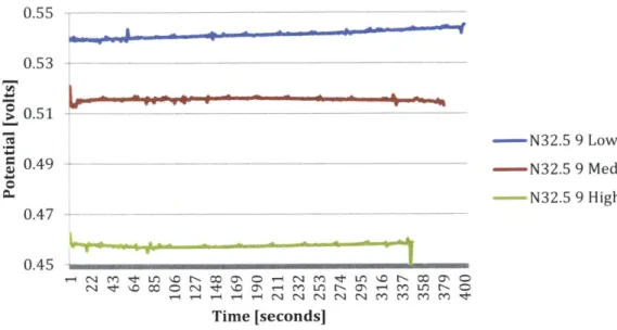
-- A M N Ct Ln \CO I- M (DI ~N Lf O ICt- CO ON C) N ~ - r- r- 0 - N rOC -4 .U .- M' M M -Rd, -N32.5 9 Low -N32.5 9 Med - N32.5 9 High Time [seconds]

Figure 11: Aside from some slight upward drift in the low and high readings, it is safe to

say that electrode N32.5 9 can be considered acceptably reliable.

N32.5 10 r- M 'C LO .O r- W 0" 0 NC W f ON C~ 0 N O 0 N , \c '. -- 0 W M LO r- r' r- M Ln N'-0 r- r-4 r 'I -4 r- N N N N N M -N32.5 10 Low -N32.5 10 Med -N32.5 10 High Time [seconds]

Figure 12: The upward drift in the low reading is slightly more pronounced than that of

electrode N32.5 9. Because of this, N32.5 10 may not be considered for implementation in the final soil analysis system electrode cartridge.

N32.5 9 0.55 0.53 > 0.51 0.49 .4-0.47 0.45 U, .1-a 0 0.54 0.52 0.5 0.48 0.46 0.44 I

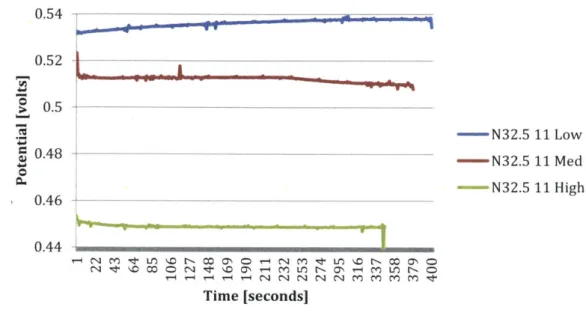
-N32.5 11 Low -N32.5 11 Med - N32.5 11 High U' N ~ Lf 'D - O Cl M~ 0 r- C31 M L r- CD~ Time [seconds]

Figure 13: The upward drift in the low reading is pronounced enough that electrode N32.5 11 probably would not be considered for implementation in the final soil analysis

system electrode cartridge.

All Electrodes Together

0.54 0.52 0.5 0.48 0.46 0.44 -N32.5 9 - N32.5 10 - N32.5 11 M \O 0" N -4 t-, 0f M? "D a, Mr in M M .I-M II It M f Ln ZO zO N- l- M a,\ 01% 0 0D r-Time [seconds]

Figure 14: Showing all three electrodes' data together is important for context and proper evaluation. From this view, we can see that all three electrodes exhibit upward drift in the low standard. Despite this, electrodes N32.5 9 or N32.5 10 would probably be the most reliable electrodes to select if necessary, as they display the most stable readings of the three. N32.5 11 0.54 0.52 0.5 0.48 0.46 0.44

All Electrodes: Soil Testing

The overall data for all electrodes taken at once, the data separated by electrode type, and the calculated soil concentration for each nutrient will be presented for each of the four soil samples tested. At the very end of this section, a master table will be provided to compare all of the calculated soil concentrations with those found in the NAPT Soil Charts [5]. As a general calculation note, all E values were calculated by taking the average value of 10 potential voltage values during a stable (no noise or drift) soil reading. All EO values were calculated by taking the average value of 20 potential voltage values during a stable low standard reading. All high potential values involved in the slope were calculated by taking the average value of 20 potential voltage values during a stable high standard reading. When reading these graphs, it should be noted that any spike in readings at the edge of a gap in data is due to the electrodes being removed from one solution and placed in another. The spike is not indicative of electrode performance, but rather a reaction from the shift in the open circuit potential system.

Kreid Soil Testing

Kreid: All Data Together 0.8 0.7 0.6 0.5 0.4 0.3 0.2 0.1 0 -0.1 -0.2

-r ~

~W~I

Figure 15: The data of all 16 electrodes was collected at once. Generally speaking, the electrodes tend to group by electrode type. Gaps in the data represent the spans of time in

0

~m.

.1-h

0

--t LA "0 r, O 0 M 00 _{C14 111Z M}

LO C) Ln 0 LO 110 r--q \ O r--I \.O \-O \D0

r--4 C14 CO LO Ln z z 00

i

which the electrodes were switched over to the next solution. The first set of data (to the left of the first gap) is the measured potential in the low standard solution, the middle data is the measured potential in the Kreid soil solution, and the third set of data is the measured potential in the high standard solution. The P3.4 series of electrodes will not be shown in greater depth, as their associated data is far too noisy and varied in drift to be of use.

Kreid: Potassium Electrodes

II

-

Figure 16: A closer look at the potassium electrodes' performance for the Kreid soil test.

This set of data appears to be rather noisy, with all three electrodes displaying drift at each stage. Initial performances like these prompted us to try conditioning new potassium electrodes in strontium chloride for later soil tests.

The calculated soil concentration for the best electrode, the K3 2.5uL 7 potassium

electrode, was 1.89 x 104. This calculation was achieved via the equations discussed in section

2.5 Simulating Soil Testing and Ideal vs. Experimental Response Theory.

The Two Point Calibration Equation was altered:

ai = 1

-4 + (E- EO)

0 s

Where a value of -4 was added to the difference in soil potential, and S was the slope between the high and low standards.

0.6 0.55 0.5 0.45 S0.4 0.35 0.3 0.25 0.2

Kreid: Nitrate Electrodes 0.8 Lt4 M DI-N N M 11 . O M~ c 0 ON r- 0D M .D~ r- r-- " N1 M M 111 --Cd M '-C %.C r. I-- M ~ 0 a, O* 0D r4 " " r- , - r-4 --N32.3 2.5 10 -N32.3 2.5 11 -N32.3 2.5 12 Time [seconds]

Figure 17: A closer look at the nitrate electrodes' performance for the Kreid soil test. Similar to the potassium electrodes, this set of data appears to be rather noisy, and also exhibits some drift (especially in the low standard and soil solution). This type of electrode was also a candidate for later strontium chloride conditioning.

The calculated soil concentration for the best electrode, the N32.3 2.5uL 10 nitrate electrode, was 5.19 x 10-5. The same equation used for the potassium electrode in the Kreid series was used for this electrode.

0.7 0.6 -. 5 e 0.4 0.3 0.2

Kreid: Phosphate Electrodes 0.5 0.45 0.4 0.35 0.3 0.25 -.

r-4 C 4 M li, O N - 00 all CD M lid L~ O %C t- 0 N Cq M ~ 14M\C

Mf

LC) LO~ 0 Lfl 0 r-4 D r-4 \.D r- 110 r- N1 N- N- CI r N Nq N-C M- M~ -RNd, LO~ Lf O %D N1 N- r O 00 0-4 (01 NOI N )

Time [seconds]

Figure 18: A closer look at the phosphate electrodes' performance for the Kreid soil test. This set of data appears to be rather noisy, and also exhibits some drift in all three solutions. This type of electrode was also a candidate for later strontium chloride conditioning.

The calculated soil concentration for the best electrode, the P2 7.9 32 phosphate electrode, was 2.33 x 10-6. This calculation was achieved via the equations discussed in section 2.5 _{Simulating Soil Testing and Ideal vs. Experimental Response Theory.}

The Two Point Calibration Equation was altered: ai =

-5 + (E- EO)

10 S

Where a value of -5 _{was added to the difference in soil potential, and S was the slope}

between the high and low standards.

-P2 7.6 11 - P2 7.6 12 - P2 7.9 32 - P2 7.9 33 0.2 0.15

Kreid: pH Electrodes --.. 0 D nr CO, - H 3.3.4 7 - H 3.3.4 8 H3.3.4 9 0 0 a -0.1 Time [seconds]

Figure 19: A closer look at the pH electrodes' performance for the Kreid soil test. This

set of data is the noisiest, and also exhibits the most amount of drift in all three solutions. This type of electrode, like the others, was also a candidate for later strontium chloride

conditioning.

The calculated soil concentration for the best electrode, the H3.3.4 7 pH electrode, was

5.71 x 10-8. This calculation was achieved via the equations discussed in section 2.5 Simulating

Soil Testing and Ideal vs. Experimental Response Theory. The Two Point Calibration Equation was altered:

-7.25 + (E- EO)

ai = 10 s

Where a value of -5 was added to the difference in soil potential, and S was the slope between the high and low standards. The slope is equal to 52 in this instance, unlike the previous three tests. 0.1 0.05 0 0 -0.05 U.15b 0% CO t- 1.0 Ln r1% C4 t- C4 r-o r-4 V-4 " r4 T-4 T-4 MA L-&--LAM4

Deckerman Soil Testing All Data Together

0.8 0.7 0.6 0.5 0.4 0.3 0.2 0.1 0 -0.1 fit-* M C -- n- -) - --+ -4 C4" M M 0'-t Oo riC4 M Time [seconds]

Figure 20: The data of all 16 electrodes was collected at once. Generally speaking, the electrodes tend to group by electrode type. Gaps in the data represent the spans of time in which the electrodes were switched over to the next solution. The first set of data (to the left of the first gap) is the measured potential in the low standard solution, the middle data is the measured potential in the Deckerman soil solution, and the third set of data is the measured potential in the high standard solution. The dip at the very end of the third set of data has been interpreted as a system error and was not sampled from for any of the final soil concentration calculations. It should be noted that the entire P3.4 series of electrodes and electrode N32.3 13 will not be shown in greater depth, as their associated data is far too noisy and varied in drift to be of use.

-K3 2.5uL 4 -K3 2.5uL 5 -K3 2.5uL 6 - N32.3 13 - N32.3 14 -N32.3 27 H 3.3.4 1 H 3.3.4 2 H 3.3.4 3 -P2 7.6 13 - P2 7.6 14 - P2 7.9 28 P2 7.9 29 P3.6 1 P3.5 2 ~m. 0

Deckerman: Potassium Electrodes 0.65 0.6 0.55 h 0.5 r 0.45 0.4 L(n 0 LO 0D LO 0D LO 0 LO~ 0 Ln 0 Lrn 0 Ln 0= n 0D Ln 0D Ln 0) LO Ln 0D -4 N.- "NM CO 1. . Ln '. 10 110 t-- r~- M M OC 0 0 r-4 N- " M T-4 1- -- -4r-4 r- r-4 Time [seconds]

Figure 21: A closer look at the potassium electrodes' performance for the Deckerman soil test. This set of data appears to be rather noisy, with all three electrodes displaying drift at the low standard and high standard. Initial performances like these prompted us to try conditioning the electrodes in strontium chloride for later soil tests. As stated before, the fourth clustering towards the end of the third set of data has been attributed to the open circuit system being bumped or an error in measurement made by the system itself.

The calculated soil concentration for the best electrode, the K3 2.5uL 5 potassium

electrode, was 1.13 x 10~4. This calculation was achieved via the same altered equation used for the Kreid potassium electrodes.

- K3 2.5uL 4 -K3 2.5uL 5 -K3 2.5uL 6 0.35

-'-~--1

Figure 22: A closer look at the nitrate electrodes' performance for the Deckerman soil

test. Similar to the potassium electrodes, this set of data appears to be rather noisy, and also exhibits some drift (especially in the high standard solution).

The calculated soil concentration for the best electrode, the N32.3 2.5uL 14 nitrate electrode, was 1.71 x 10-3 . The same equation used for the potassium electrode in the Deckerman series was used for this electrode.

Deckerman: Nitrate Electrodes

Deckerman: Phosphate Electrode 0.55 0.5 0.45 S0.4 0.35 0.3 0.25 0.2 0.15 0.1 I 4_4 _ _ _ _

I

Figure 23: A closer look at the phosphate electrodes' performance for the Deckerman

soil test. This set of data appears to be quite noisy, but the performance of each electrode is at least similar to that of one another. This type of electrode was also a candidate for later strontium chloride conditioning.

The calculated soil concentration for the best electrode, the P2 7.9 29 phosphate electrode, was 4.01 x 10-4. This calculation was achieved via the same altered equation used for the Kreid phosphate electrodes.

-P2 7.6 13 -P2 7.6 14 - P2 7.9 28 P2 7.9 29

Deckerman: pH Electrodes

Iii

I

~Ii___

LI

Figure 24: A closer look at the pH electrodes' performance for the Deckerman soil test. This set of data is noisy, much like the Deckerman potassium data. It also exhibits drift in all three solutions. This type of electrode, like the others, was also a candidate for later strontium chloride conditioning.

The calculated soil concentration for the best electrode, the H3.3.4 1 pH electrode, was

5.39 x 10~ . _{This calculation was achieved via the same altered equation used for the Kreid pH}

electrodes. 0.2 0.15

Darroch Soil Testing All Data Together

p

_____i

.4: .4:.4:

Figure 25: The data of all 16 electrodes was collected at once. Starting with Darroch soil testing, we decided to use electrodes conditioned in strontium chloride during fabrication to see if the electrode responses would be more reliable (drifting less) and less noisy (stable in general). It should be noted that the electrodes with an 'S' listed in their name were conditioned in strontium chloride, while electrodes with a '*' listed in their name are regular electrodes that were not conditioned in strontium chloride (like the electrodes used in the Kreid and Deckerman tests were). Aside from some obvious outliers, it appears that conditioning the electrodes in strontium chloride was beneficial. It should be noted that electrode P2 7.9 20m 5 is not further analyzed in the P2 7.9 20m series because

it is far too noisy of data to be useful.

-N32.6 S10 - N32.6 S11 -N32.6 S12 N32.2 *4 - H3.3.4 S4 - H 3.3.4 S5 H3.3.4 S6 - pH 3.3.4*1 - P2 7.9 20m 3 - P2 7.9 20m 4 P2 7.9 20m 5 - P2 7.9 20m 6 0.2 0 4.) 0 -0.1 -A2, - ~. VA*Am*Awb

jPqPP-Darroch: Potassium Electrodes 0.45 0.4 0.35 0.3 0.25 0.2 AL o r1 t - M~ M N "t M r- - M M ltd Uct M N-1- " M ' Lf ,-I

a- doo - r- .oC Lfn L 4 -td co Nq cn -4 00 =~ d a- co do-,

Time [seconds]

Figure 26: It appears that the potassium electrodes conditioned in strontium chloride are

far less noisy than the potassium electrodes in the Kreid and Deckerman trials were. It makes sense that K3 *3 would be an outlier in this experiment, seeing as it is the only electrode that wasn't conditioned in strontium chloride. The potassium electrodes in general could still be improved in stability (drift) and reliability (consistent reading per electrode group type), but this initial graph seemed like a step in the right direction.

The calculated soil concentration for the best electrode, the K35 S 12 potassium

electrode, was 1.09 x 10-4. This calculation was achieved via the same altered equation used for

the Kreid and Deckerman potassium electrodes.

- K35 S 10

-K35 S 11

-K35 S 12 -K3 *3

Darroch: Nitrate Electrodes 0.5 0.48 0.46 0.44 F-o rN Lfn " l N O Rr1 N' M -_ M~ MD M~ V4 cr, ~ M O ' "0 M ' -4= 7,M rr M ~ ~ ~ ~ ~ -1-1,-%Or MC%01 Nn " - 14" " 01%11 CON Time [seconds]

Figure 27: This data is the most promising-looking set of data we have seen so far. It

makes sense that the N32.2 *4 (non-conditioned) electrode is the outlier. As for the three other electrodes, they are closely grouped together, which bodes well for reliability. The lack of noise in these plots is also an improvement. Upon closer inspection, however, it appears that the low and high standard data are not quite 0.1 volts apart. We will be able to tell more once we compare the actual Darroch nutrient measurements with these specific potential voltage readings (see Table 4 on page 46).

The calculated soil concentration for the best electrode, the N32.6 S12 nitrate electrode,

was 1.66 x 105. The same equation used for the potassium electrode in the Darroch series was

used for this electrode.

-N32.6 S10 - N32.6 S11 -N32.6 S12 - N32.2 *4 0.42 10.4 0.38 0.36 0.34 0.32 0.3

_____________________ _F r-4 r- '- I-- P2 7.9 20m 3 --- P2 7.9 20m 4 - P2 7.9 20m 6 Time [seconds]

Figure 28: P2 7.9 20m 3 appears to be an outlier of the group. P2 7.9 20m 6 is a little too

noisy to be considered a useable electrode for the final soil analysis cartridge. The low and high standard solutions for these electrodes do not appear to be 0.1 volts apart, so the subsequent soil concentration calculation is probably not within the range of what the Darroch soil was actually measured to be.

The calculated soil concentration for the best electrode, the P2 7.9 20m 3 phosphate electrode, was 1.24 x 10-7. This calculation was achieved via the same altered equation used for the Kreid and Deckerman phosphate electrodes.

Darroch: Phosphate Electrodes

0.4 0.38 0.36 0.34 0.32 S 0.3 * 0.28 0.26 0.24 0.22 0.2

C14 It I'D W 0* r-I MY) Ln

r--: L6 r 14 C C6 16 4

M tl- 110 Ln M C14 r-4 CD

Ln %.C rI_ M a's CD