Optimal configuration of active-control mechanisms

Publisher’s version / Version de l'éditeur:

Journal of Engineering Mechanics, 120, 3, pp. 535-556, 1994-03

READ THESE TERMS AND CONDITIONS CAREFULLY BEFORE USING THIS WEBSITE.

https://nrc-publications.canada.ca/eng/copyright

Vous avez des questions? Nous pouvons vous aider. Pour communiquer directement avec un auteur, consultez la

première page de la revue dans laquelle son article a été publié afin de trouver ses coordonnées. Si vous n’arrivez pas à les repérer, communiquez avec nous à PublicationsArchive-ArchivesPublications@nrc-cnrc.gc.ca.

Questions? Contact the NRC Publications Archive team at

PublicationsArchive-ArchivesPublications@nrc-cnrc.gc.ca. If you wish to email the authors directly, please see the first page of the publication for their contact information.

NRC Publications Archive

Archives des publications du CNRC

This publication could be one of several versions: author’s original, accepted manuscript or the publisher’s version. / La version de cette publication peut être l’une des suivantes : la version prépublication de l’auteur, la version acceptée du manuscrit ou la version de l’éditeur.

For the publisher’s version, please access the DOI link below./ Pour consulter la version de l’éditeur, utilisez le lien DOI ci-dessous.

https://doi.org/10.1061/(ASCE)0733-9399(1994)120:3(535)

Access and use of this website and the material on it are subject to the Terms and Conditions set forth at

Optimal configuration of active-control mechanisms

Abdel-Mooty, M. A. N.; Roorda, J.

https://publications-cnrc.canada.ca/fra/droits

L’accès à ce site Web et l’utilisation de son contenu sont assujettis aux conditions présentées dans le site LISEZ CES CONDITIONS ATTENTIVEMENT AVANT D’UTILISER CE SITE WEB.

NRC Publications Record / Notice d'Archives des publications de CNRC:

https://nrc-publications.canada.ca/eng/view/object/?id=d4b7f56c-4114-4c20-9ed2-ec660338facc https://publications-cnrc.canada.ca/fra/voir/objet/?id=d4b7f56c-4114-4c20-9ed2-ec660338facc

Opt im a l c onfigura t ion of a c t ive -c ont rol m e c ha nism s

N R C C - 3 6 0 4 1

A b d e l - M o o t y , M . A . N . ; R o o r d a , J .

M a r c h 1 9 9 4

A version of this document is published in / Une version de ce document se trouve dans:

Journal of Engineering Mechanics,

120, (3), pp. 535-556, March-94, DOI:

10.1061/(ASCE)0733-9399(1994)120:3(535)

http://www.nrc-cnrc.gc.ca/irc

The material in this document is covered by the provisions of the Copyright Act, by Canadian laws, policies, regulations and international agreements. Such provisions serve to identify the information source and, in specific instances, to prohibit reproduction of materials without written permission. For more information visit http://laws.justice.gc.ca/en/showtdm/cs/C-42

Les renseignements dans ce document sont protégés par la Loi sur le droit d'auteur, par les lois, les politiques et les règlements du Canada et des accords internationaux. Ces dispositions permettent d'identifier la source de l'information et, dans certains cas, d'interdire la copie de documents sans permission écrite. Pour obtenir de plus amples renseignements : http://lois.justice.gc.ca/fr/showtdm/cs/C-42

OPTIMAL CONFIGURATION OF ACTIVE-CONTROL MECHANISMS"

By Mohamed Abdel·Mooty1 _{and John Roorda}2

ABSTRACT: The relative merit of the different control.configurations cannot be foreseen by considering only the controllability and observability .conditions. A measure of the degree of controllability has to be defined to help choose the best control configuration. The optimal control configuration that maximizes the control effectiveness and minimizes the control cost is considered in this paper. The vi-brational mode shapes, the structure-controller interaction, the control strategy, the control objective, and the control spillover are among the factors influencing the optimal placement of the control actions. The contribution of these factors in the control distribution problem is assessed through numerical examples.lt is found that the structure-controller interaction, a factor usually neglected in previous stud-ies, greatly affects the optimal control distribution. Quantitative measures of the degree of controllability are proposed. Finally the paper presents a methodology for dealing with the optimal control configuration problem, a problem that does not have a unique solution.

INTRODUCTION

According to modern control theory, a general rule for placing a limited number of sensors and control actions on a continuous structure is to satisfy the observability and controllability conditions for the controlled modes. However, for a given control configuration, this criterion tells only whether. the structure is controllable or not. The relative merit of the different control configurations cannot be foreseen by considering only the ccintrollability and observability conditions. A measure of the degree of controllability has to be defined to help choose the best control configuration. In the present paper, an effort is made to define a scalar controllability measure or degree of controllability (DOC). This measure should have the following attributes:

It must vanish for uncontrollable structure

• It must indicate the control effectiveness, which is the ability of the control to induce the desired effect

It must indicate the control cost as a measure of the effort made to achieve the required control level

It must reflect the control objective, whether it is control for the safety of the structure, for the comfort of the users, or for the sensitive operation of the secondary systems mounted on the struc-ture

"Part of this work was ｰｾ･ｳ･ｮｴ･､＠ at the ASCE Engineering Mc::chanics Speciality Conference, Columbus, Ohio, May 19-22, 1991.

1_{Res. Assoc., lost. for Res. in Constr., Nat. Res. Council Canada, Ottawa, On·}

tario, Canada KIA OR6; formerly, Post-Doctoral Fellow, Civ. Engrg. Dept., Univ. of Waterloo, Ontario, Canada.

2_{Prof., Civ. Engrg. Dept., Univ. of Waterloo, Waterloo, Ontario, Canada N2L} JGI.

Note. Discussion open until August 1, 1994. To extend the closing date one month, a written request must be filed with the ASCE Manager of Journals. The manuscript for this paper was submitted for review and possible publication on October 7, 1992. This paper is part of the Journal of Engineen"ng M11chanics, Vol.

llfb.No

3 March 1994. ©ASCE, ISSN 0733-9399/94/0003-0535/$2.00

+

$.25 per page. Paper No. 4916.

At this point, it is necessary to stress that the optimal configuration of the control mechanism is problem-dependent. It varies for different control mechanisms, algorithms, and objectives as well as loading. The optimal position for an active mass damper may not be optimal for an active tendon or pulse generator. The way the control system works, whether open-loop, closed-loop, or open-closed-loop, has an impact on the optimal placement of the control action. The optimal placement of the control actions greatly depends on the control objective. Control for safety aims at limiting the relative displacements of the different points on the structure while control for comfort is to limit the absolute acceleration. Finally, since structures respond differently to the large spectrum of external excitations, such as earthquakes, wind, waves, traffic, impact, etc., the load that mainly affects the structure and necessitates the control application would have an influ-ence on the best distribution of the control actions.

The work in the present paper aims at investigating, for a particular structure and control mechanism using closed-loop control strategies and given control objective, the other factors that govern the optimal distribution of the control actions. The structure considered here is a simple beam, modeling a single span bridge, controlled by an active tendon mechanism. The most important factor affecting the optimal control configuration is the vibrational mode shapes of the controlled modes because a mode becomes uncontrollable if the control force is placed at its nodal point. Another factor, considered here and usually neglected in previous studies, is the interaction between the original structure and the control mechanism. Two different control strategies, namely direct velocity feedback (DVFB) control and linear quadratic optimal control (LQOC) are considered. Finally the effect of control spillover into the uncontrolled modes on the optimal dis-tribution of the control actions is considered.

To implement the DOC defined before, quantitative measures of both the control effectiveness and cost must be defined first. The main objective of the control is to keep the structural motion (displacement, velocity, and/ or acceleration) as small as possible during the excitation and to bring the structure to rest as fast as possible after the excitation. This can be achieved by introducing active stiffness and active damping to the structure. However, since large structural motions occur near resonance and the excitation fre-quency and time history are, in general, not known in advance it is more effective to rely on the active damping in controlling the structure. The amount of damping in a certain mode gives a good indication of how fast . that mode comes to rest in free vibrations as well as the maximum response amplitude during its forced vibrations. Therefore the amount of active damp-ing in a certain mode is chosen as a measure of the control effectiveness in that mode. The control effort is subject to limitations on the available actuator force, stroke, hydraulic power, and delivery rate. The maximum actuator force, ram displacement, power, delivery rate, or the total control energy used during the control implementation can be used as measures of the control cost. These measures are closely related and most of them are examined in the present study. Both control effectiveness and cost depend very much on the location of the control actions on the structure. The best

control configuration is the one that maximizes the control effectiveness

and minimizes the control cost. ·

In the present paper a control efficiency measure, for each controlled mode, defined as the ratio of the active damping to the control effort utilized to achieve that damping is considered as a candidate for the required degree

of controllability. The effect of the control strategy and control mechanism on that measure is studied. An effort is made to .arrive at an integrated control efficiency measure that includes the contributions of all the con-trolled modes and reflects the control objective. But first, the previous studies in this area are briefly reviewed.

LITERATURE REVIEW

Among the first attempts to address the degree-of-controllability issue was the work of Kalman et al. (1963), in which a symmetric controllability matrix for time-varying linear systems was defined. That study further de-fined the determinant and the trace of that matrix as scalar measures of the controllability. Arbel (1981) used the controllability definition of Kalman et al. (1963) and added the minimum eigenvalue of the controllability matrix as a third measure of controllability. Although those measures vanish when the system becomes uncontrollable, it is not clear what other physical mean-ing can be related to the eigenvalue, trace, or determinant of the control-lability matrix.

Juang and Rodriguez (1979) defined, within the framework of the optimal control theory for systems subjected to initial disturbances, the value of the cost function that is to be minimized as an indication of the controllability. They defined the optimal actuator distribution as the one that makes the cost function an absolute minimum.

Hughes and Skelton {1979) used the norms of the rows of the control location matrix as measures of the controllability of the individual modes. Vilnay (1981) and Ibidapo-Obe (1985) studied the functional relationship between the actuator location and the structural mode. In an attempt to consider the control effort in the actuator placement, Abdei•Rohman {1984) suggested that the optimal distribution of the sensors and the actuators is that which minimizes the observer gains and the control gains for the same level of control. However the control gains do not represent completely the control effort, which depends greatly on the type and configuration of the control mechanism.

The optimal actuator placement in controlling large structures in space subjected to initial disturbances was considered in-Viswanathan et al. (1979), Lindberg and Longman (1981), Longman and Lindberg (1986), Viswana-than and Longman (1983), and Longman and Horta (1989). A recovery region in the state space was defined as the region that includes all of the initial conditions (or disturlled states) that can be returned to the origin (rest) in a finite time T using the bounded control forces. The degree of controllability was defined as a scalar measure of the size of the recovery region. Longman and Horta (1989) showed that actuator masses may have a significant effect on the optimal actuator placement when they are large compared with the structural mass.

In an attempt to define a degree of controllability for seismic buildings, Cheng and Pantelides (1988) suggested a weighted sum of the squares of the modal displacements at the actuator position, each multiplied by the maximum modal response spectrum value for the design earthquake. How-ever this criterion does not satisfy the basic requirement that the DOC vanishes when the system becomes uncontrollable. In a deviation from the concept of the degree of controllability, Chang and Soong (1980) considered the optimal controller placement that minimizes a weighted sum of the squares of the control forces for the same level of co"trol. Schulz and

Heimbold (1983) presented a method based on the maximization of the energy dissipated due to the control actions.

The problem of optimal actuator locations was also tackled within the framework of combined structural and control optimization. Haftka and Adelman (1985) considered the problem of selecting

n

actuator locations from a set of m available sites, m

>

n, for static shape control of large space structures. Onoda and Haftka (1987) considered simultaneous optimization of structural and control systems for flexible spacecraft for a given distur-bance. Cha et al. (1988) considered the minimization of the structural re-sponse, the control force, and the structural weight as an application of the general theory of optimal control of parametric systems. They allowed the actuator position to be a design variable and the optimal location for min-imum cost was obtained for given disturbance. Khot et al. (1990) considered the optimum number of actuators and their locations with the objective of minimizing the weight of the structure and satisfying constraints on the closedcloop eigenvalues for a specified disturbance .

• 1 MATHEMATICAL MODEL

i:!.

' 1, The structure considered for active control application is a simply sup-ported beam modeling a single-span bridge. The structural dimensions used in the present paper are those used in experimental studies on active struc-tural control by the writers (Abdel-Mooty and Roorda 1991a, d). The beam span I is 5 m, mass per unit length m is 12.2 kglm, and bending stiffness EI

is 133,000 N X m2 (Fig. 1). The control force is applied through a post by the action of pulling or releasing a cable of axial stiffness, EA = 730 kN, by means of a hydraulic actuator. The post of mass M = 1.577 kg and length el = 0.5 m is placed at distance gl from the left support, where 0

<

ｾ＠

<

1.0. The equation of motion and the boundary conditions for the un-damped free vibration of the beam-post-cable arrangement reads

EJwiV(x, 1)

+

KB(x - gl)w(x, 1)

+

mw(x, 1)

+

MB(x - gl)w(x, 1) = 0

... (1) w(O, 1) = w"(O, t) = w(l, 1) = w"(l, t) = 0 ... (2) where w(x, t)

= beam displacement at any point x and at any timet; primes

denote derivatives with respect tox; overdots denote derivatives with respect to

t;

3 = Dirac delta function; and K is the passive stiffness of the control . mechanism at the post location, defined as the force acting on the beam at

Actuator

FIG. 1. Active Tendon Control of Bridge-Like Structures

the post due to unit displacement of the beam at the post. As well, K is a function of the material and the geometric characteristics of the cable.

The natural frequencies w, and the mode shapes of vibrations Y,(x) can be obtained by solving (1) and (2) using Galerkin's approach as in Abdel-Mooty and Roorda (1991b) or any other numerical technique. The vibra-tional modes Y,(x) are normalized to satisfy the orthonormality condition

r

.

Jo

NY.(x)Yi(x) dx

=

B,i ... (3) where B,i = Kronecker's symbol and N = mass operator given by

NY(x) = mY(x)

+

MB(x - ｾｬＩｙＨｸＩ＠ ... (4) The next step is to consider the dynamics of the whole system governed by the following equation of motion:

EfwlV(x, t)

+

KB(x - ｾｬＩｷＨｸＬ＠ t)

+

Cw(x, t)

+

Nw(x, t) = f(x, t)

+

Sv(t)B(x - ｾＯＩ＠ ... (5) and the boundary conditions given by (2). In (5), C = damping operator assumed to be of the proportional viscous type;f(x, t) = external excitation;

v(t)

=

actuator movement; and S

=

active stiffness of the control mechanism at the post. The variable S is the force acting on the beam at the post due to a unit displacement of the actuator shaft, and it is a constant dependent on the material and geometric characteristics of the cable.i The solution of (5) can be written as

"

w(x, t) =

2:

ui(t)Yj(x) ... (6)

i"" 1

where the coordinate functions Yj(x) = orthonormal mode shapes of the original structure with the control mechanism in place. Using (6) in (5), multiplying by Y.(x), integrating over the length of the beam, and observing the orthonormality condition results in

a,(t)

+

2,,w,u,(t)

+

wlu.(t) = [,(t)

+

ｓｙＬＨｾｬＩｶＨｴＩＬ＠ k = 1, 2, 3, ... , oo ... (7)

i

l .

f,(t)

=

Y,(x)f(x, t) dx ... (8)

0 .

and '' = damping ratio in the kth mode.

CONTROL MECHANISM EFFECT

In most of previous studies, control actions were regarded as individual

forces or moments applied at different points on the structure. In reality, these forces can only be applied through the use of control mechanisms that cause changes in the structural parameters even when they are not activated. The interaction between the control mechanism and the original structure, and its effect on the optimal configuration of the control mechanism, is the focus of the present section. .

The tendon control mechanism apds to the original beam a point mass

Mat the post position. Furthermore, the motions of both the beam and the 539

.

'

ｾ＠

ｾ＠

ｾ＠

i

_E

ﾷｾ＠

_<U

.s::

&l

E

e

_....

c:

0

u

FIG. 2. 200 100

passive stiffness at the post

passive stiffness at the actuator

active stiffness at the post

active stiffness at the actuator

ＰｾｾＭＭｲＭＭＭＭＭｲＭｾＭＭｲＭｾＭＭｲＭＭＭｾ＠

0 1

2

3

4

5

Control force position {m)

Control Mechanism Stlffnesses for Different Control-Force Positions

actuator shaft generate forces in the cable with components. applied to the beam at the post and to the actuator. These forces are functions of the material and geometric characteristics of the cable. Cable forces due to the beam motion are called passive forces and those due to the actuator move· ment are called active forces. These interactive forces are characterized by the passive stiffness of the control mechanism at the post and at the actuator

K and K, respectively, and the active stiffness of the control mechanism at

the post and at the actuator S and cr, respectively. The passive stiffnesses are the forces, applied to the beam at the post or to the actuator, due to unit displacement of the beam at the post while the active stiffnesses are the forces due to unit displacement of the actuator shaft. The calculated stiffnesses for different control configurations are shown in Fig. 2.

It should be noted that the variations of the passive and active. forces acting on the beam with the different control-force positions are significantly different from those acting on the actuator shaft. The forces acting on the actuator should be the ones used in evaluating the control effort. The use of the control force acting on the structure as a measure of the control cost can be misleading.

The presence of the control mechanism, even when it is not activated,

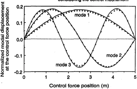
changes the free vibration characteristics of the original structure. The nor· malized modal displacements at the post position for different control mech· anism configurations considering the cori.trol mechanism effect are ｣｡ｬ｣ｵｾ＠

lated, using Galerkin's approach as in (Abdel-Mooty and Roorda 1991b), and compared with those of the original structure. Fig. 3 shows the passive effect of the control mechanism on the first three vibrational mode shapes. It is clear that the existence of the control mechanism does change the vibrational mode shapes of the original structure. This effect could be sig·

neglecting the control mechanism

considering the control mechanism

0.1

-0.1

ＭＰＮＲＱＭｾＭＮＭＭｾＭＮＭＭｾＭＮＭＭｾＭＮＭＭｾＭＭｬ＠

0 1 2

3

4

5

Control f.orce position (m)

FIG. 3. Normalized Modal Displacements at Post for Different Control Conflgu·

ration

nificant if the stiffnesses and masses added by the control mechanism were relatively large compared with those of the original structure. However, for the mechanism considered here, this effect is relatively small.

MODAL CONTROL EFFICIENCY INDEX

The equation of motion of the actively controlled structure using a single control force reads

u/t)

+

2'

₁wi";(t)

+

wfu

1(t) = Jj(t)

+

ｓｙ _Ｑ ＨｾｬＩｶＨｴＩＬ＠ j = 1, 2, 3, ... , n ... (9) · where n = number of controlled modes and the different variables in (9) are as defined in (7). Eq. (9) is externally coupled because the actuator movement v(t), in general, depends on a full complement of the state var-iables u₁(t) and

u

₁(t), j = 1, n. Coupling causes a small shift in the closed· loop poles designed for the uncoupled system; particularly for systems with well separated vibrational modes as the one considered in the present paper (Abdei-Mooty 1992). This coupling will be neglected and the control will be designed for each mode independently. This approximation allows for the derivation of closed-form solutions for the closed-loop poles which gives more insight into the variation of the control efficiency with the control force position.

In this section, the active damping coefficient in each controlled mode is calculated as a measure of the control effectiveness in that mode. The direct velocity feedback control and the linear quadratic optimal control are used to show the effect of the control strategy on the control efficiency. The total (active plus passive) actuator force utilized in controlling a certain mode is used as a measure of the control cost in that mode. A control efficiency

541

i

!

i,ndex is defined, for each mode, as the ratio of the control effectiveness to the control cost.

Direct Velocity Feedback Control

The velocity sensed at the control force location, multiplied by a negative gain G, is used directly as the feedback signal to the actuator movement. This gives the active damping coefficient for the jth mode

cA,

as (Abdel-Mooty and Roorda 1991a)

1

cA,

=

z

GSYJW) ... (10)

The total control force used in achieving the above damping is composed of the active actuator force due to the actuator shaft movement fA. and the passive actuator force due to the beam motion fp. These forces, for the jth

mode, are given by , 1

fA1 = - ｇ｡ｙ _Ｑ ＨｾｬＩｵ _Ｑ ＨｴＩ＠ ... " ... (11)

fp₁ = - KlfW)u₁(t) ... (12)

In (10)-(12) the different stiffnesses, K, S, and a, of the control mechanism

are functions of the control force position ｾＱＮ＠ The total control force in the jth mode is

fi

= ｇ｡ｙ

_Ｑ

ＨｾＱＩｵ

_Ｑ

ＨｴＩ＠

+

KY₁W)u₁(t) ... (13a) To facilitate the subsequent manipulations the total control force is written, approximately, in terms of the modal velocity coordinate ll₁(t) as

fi

= ( Ga ±

ｾＩ＠ ｙ

Ｑ

ＨｾＱＩＱｬｪＨｴＩＬ＠

i =

v"=1 ...

(13b) For simplicity let the time independent control force index for the jth mode,

[₁₁, be defined as

[ 11 =

I

ｙ

Ｑ

ＨｾＱＩ＠

Ja'a'

+ :;/ ...

(14) Since the total actuator force for the jth mode, is calculated in terms of the. modal velocity coordinate ll₁(t), of that mode, the relative magnitudes of the control force indices for the different modes will depend on the relative magnitudes of their controlled modal velocities

u

₁(t), j = 1,

n.

Dividing the active damping coefficient by the control force index yields the modal control efficiency index for the jth mode, ｍｃｅｉ _Ｑ ＨｾＱＩＬ＠ as

2

Ja'a'

+

ｾ＠

_wJ

... (15)

where ｾｉ＠ = control force position measured from the left end. This measure· indicates the amount of active damping introduced to the jth mode per unit control force. Therefore it is considered as the DOC of that mode. As can be seen from (15) the distribution of this DOC depends not only on the vibrational mode shapes but also on the distribution of the different control

mechanism stiffnesses. The variation of the control effectiveness indices (active damping coefficient), control force indices, and control efficiency indices for the first three modes with the different control force positions are shown in Figs. 4, 5, and 6. In calculating these measures the DVFB gain G is assigned arbitrarily the value of 0.005.

Linear Quadratic Optimal Control

Once again the coupling between the controlled modes is neglected to obtain form approximate mathematical expressions for the closed-loop poles using the LQOC strategy. The control gain for the jth mode using linear optimal control strategy is designed such that the following quadratic performance index J is minimized:

J =

J: {

ＨｾＩＧ＠ ｛ｾｉ＠ ｗｾｷｊ｝＠

ＨｾＩ＠

+

vrav} dt ... (16)

where t₁ = terminal control time, which is larger than that of the excitation; and ltj = a weight factor assigned to the jth mode. This minimizes a weighted sum of the total energy in the structure and the control energy. The min-imization of the cost function (16) yields the optimal! x 2 feedback control gain row vector G

p G = br- ... (17a) (1 ' ' b

=

' ... ' ' ... ' ... ' .. '' ' ... (17b) P= [P1 _P2 ] P2 P3 ... (17c)

where b = control location vector; and P = a 2 x 2 symmetric positive semidefinite matrix that satisfies the nonlinear matrix Riccati equation

(Bry-son and Ho 1975). The optimal actuator movement is given by

v(t) = G

Ｈｾ［Ｉ＠

... (18) Using (17) in (18) yields the active actuator force fA, as

fA, = Slj(t/)[P,u₁(t)

+

P2

u

1(t)] ... (19) where P1 and P2 = elements of the Riccati matrix given by (Abdel-Mooty

1992)

P2 =

[-I

+

1

+

S'YJW)W] 2 I S' w'a ',(<f) ... ' .. ' .. ' .... ' .... (21)

W;f1 Y; ':.

For the system considered here, ＨｓＧｹｙＨｾｬＩｗＩｉＨｷｪ｡Ｉ＠

<<

1. Therefore 543

I

ｾ＠

r

I

I

r

I

I

I, !

I

,<

'

w

P₂ = ｾ＠ , , , , , , , , , , , , , , , , , , , , , , , , , , , , , , , , , , , , , , , , , , , , , , . , , . , (22) Using (17), (18), (20), and (22) in the closed-loop system equation (9) yields

1

₊

S'YJW)W; . _ ( 2 S'YJW)W1) = [,- (₂₃₎

2 z z uJ

+

w,

+

ui ' ...

t1w1rr 2rr

The closed-loop poles for the jth mode are given by

1

+

ｓＧｙｾＨｾ［Ｉｗ［＠

± iw₁

vr=-v , ... , .. , ... , ,

(24)

2,/W/<T

The active damping coefficient in the jth mode cA- is

I

cA,

=

SY₁

W)

ｾＭ

. -- ... -- ... -- -- .. -- . -- -- .. _. -- ...

(25) The active actuator force for the jth mode is given by (19) while the passive actuator force is given by (12). The total control force index for the jth

mode /1 is approximated by

I

, !I,=

ll)W)

S'Pl

+

(SP,w;

KYI·'".'" '" ... '" ... '"'" ..

(26) Therefore the modal control efficiency index for the jth mode, ｍｃｅｉ _ＱＨｾＯＩＬ＠

is

' ... ' .. '' .... (27)

The variation of the control effectiveness indices (active damping coef-ficients), the control force indices, and the control efficiency indices for the first three modes with the control force location are shown in Figs. 4-6, The value assigned for the weighting factors W_1, j = 1, 2, 3, in (25)-(27)

is 'chosen, after some trials, as 0.053, which gives approximately the same

level of damping obtained earlier for the DVFB control strategy.

The significant effect of the vibrational mode shapes on the active damping coefficients, using DVFB and LQOC strategies, is shown in Fig. 4, Maxi-mum damping values occur near the points of maxiMaxi-mum modal displacement while points of zero damping coincide with the nodal points. The correlation between the distribution of the modal displacements and the active damping coefficients is slightly distorted by the effect of the control mechanism stiff-nesses. High values of damping, for the same control gain, are achieved near the ends of the beam following the distribution of the active stiffness of the control mechanism at the post (Fig. 2). Also the -unsymmetric dis-tribution of the active stiffness of the control mechanism is reflected on the active damping distribution.

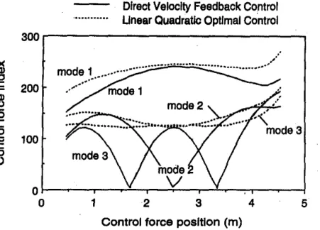
Fig. 5 shows higher control force index for the first mode than those for 544

Direct Velocity Feedback Control

j

12

Unear Quadratic Optimal Control mode3 ｾ＠

₁₀

'-'

'C

Q)

8

'l.i

s

8

6

01

4

.5

a.

ｾ＠

2

ｾ＠

0

'il

0

<( 1

2

3

4

5

Control force position (m)

FIG. 4. Active Damping Coefficients for Different Controi·Force Positions

ｾ＠

Direct Velocity Feedback Control Unear Quadratic Optimal Control

ＳＰＰＮＭＭＭＭＭＭＭＭＭＭＭＭＭＭＭＭＭＭＭＭＭＭＭＭＭＭＭｾ＠

.5

200

ｭｯｾｾ｟Ａ＠

... / /

ｾ＠

.e

:g

c:

100

8

ｯｾｾＭＭｲＭｾｾｲＭｾＭＭｲＭｾｾｔＭｾｾ＠ 0 1

2

3

4

5

Control force position (m)

FIG. 5. Modal Control-Force Indices for Different Control-Force Positions lhe second and third mode. That is because, for the same modal velocity coordinate tl;(l) for all modes, the modal displacement coordinates u;(t) for the lower modes are larger than those for the higher modes, as long as w;

> 1 rad/s. Since the passive actuator force [see (12)] is proportional to the modal displacement, the total (active and passive) control force is expected

545

'

Direct Velocity Feedback Control

Unear Quadratic Optimal Control

0 . 1 0 r - - - , 0.08

·· mode3

..

0.06 0.04

0'02

ｭｯ､ｾﾷｲﾷﾷﾷ＠

....

ﾷﾷＮＺＮＺﾷﾷｾﾷﾷ［［ｯﾷﾷＮＮＮｲｲＮ｣ＭＭＭｴｾｾ＠

-0.00 ＱＭｾＭＮＮＭＭｾＭＢＭＮＮＮＬＮＮＮＮＮＮＭＭＧＴＢＭＭｲＭＭＢＭｾＭＮＭＭｾｾ＠ 0 1 2 3 4 5

Control force position (m)

FIG. 6. Modal Control Efficiency Indices for Different Control Force-Positions

to be higher for the lower modes assuming the same modal velocity for all modes. This consequently leads to a lower control efficiency index for the lower modes. If the amplitudes of the modal velocities are expected to be different in the controlled response, the control efficiency index for the different modes shown in Fig. 6 must be multiplied by different weighting factors to account for their relative modal velocity amplitudes.

Also, Fig. 5 shows, in general, higher control force indices at the right end of the beam. This follows from the distribution of the active and passive stiffnesses of the control mechanism at the actuator, Fig. 2. The effect of the unsymmetrical distribution of the control mechanism stiffnesses is re· fleeted in the distribution of the modal control efficiency indices, Fig. 6. Fig. 6 shows that the control strategies used may have a small effect on the control efficiency. However these small differences due to the use of dif· ferent control strategies are unlikely to affect significantly the optimal dis· tribution of the control actions.

OPTIMAL CONFIGURATION CRITERION

The modal control efficiency index derived in the previous section, in fact, is a scalar measure of the degree of controllability for each individual

mode. This measure satisfies the basic requirements mentioned in the

in-troduction of the present paper. It vanishes when the mode becomes un-controllable; it indicates the control effectiveness in terms of the active damping coefficient introduced to that mode; and also it indicates the control effort represented by the control force. It remains to define a controllability measure that includes the effect of all the controlled modes collectively. That measure should reflect the effect of the exciting loads as well as the overall control objective whether for safety, comfort, or secondary system operation.

Different candidates for the DOC measure are proposed in this section 546

and evaluated numerically in the next section. The optimal control config-uration is the one that maximizes the DOC. The first controllability measure follows from the fact that the structure becomes uncontrollable when any of its modes that are supposed to be controlled becomes uncontrollable. That is, the controllability of the structure is limited by the controllability of the least controllable mode. Based on that, the first controllability mea-sure (DOC!) is defined as

DOC! =

m:n

｛ｍｃｾ［ＨｻｉＩ＠

J ...

(28) where MCEI;({I) = modal control efficiency index for the jth mode, and

U;, j

=

I,

n,

are modal weighting factors. The choice of U; should reflect the effect of the loading and the control objective as illustrated in the next section. If all controlled modes are of the same importance and if the controlled modal velocity coordinates it;(t) are expected to be of the same order of magnitude the modal weighting factors will all be equal to 1.0. Fig. 7 shows the variation of DOC! with the control force position for unit U;,

j = I,

n,

using DVFB control strategy.

'According to DOC!, the optimal control force location is the one that maximizes the minimum modal controllability. Obviously this definition does not include the effect of all the modes collectively whereas the structural

motion contains contributions from all the vibrational modes

simultane-ously. To overcome such shortcoming a second controllability measure is proposed. Since the control aim is to limit the vibrations of all the controlled modes by maximizing, simultaneously, the active damping in the controlled modes, a suitable controllability measure may be defined as

n

DOC2 =

2,;

U;MCEI;({I) ... (29) j""l

where

U;

= modal weighting factors defined previously. One may argue that since the maximum modal control forces for the controlled modes do not all occur at the same time, the controllability measure should be defined as

n

DOC3

=

2,; (

ｖ［ｍｃｅｉ［ＨｾＯＩＩ Ｒ＠ _{• • • . • • • • • • • • • • • • • • • • • • • • • • • • • • • (30)}

j= I

Fig. 7 shows the controllability measures DOC2 and DOC3 for different control force positions assuming the value of 1.0 for U;, j = I, 2, 3.

Both controllability measures DOC2 and DOC3, although they include the effect of all controlled modes, do not vanish when the system becomes uncontrollable. The direct use of these measures in optimal actuator place-ment may lead to an uncontrollable system. For example, if the first three modes are to be controlled with the same weight and if the control force location is restricted to ihe middle third of the beam, according to DOC3 of Fig. 7, the optimal location is at the midspan point. However, for this configuration the second mode and consequently the whole system is un-controllable. Therefore one has to keep an eye on the controllability of the least controllable mode, i.e. DOC!, and at the same time consider the contribution of all the modes, i.e. DOC2 or DOC3. This can be achieved by imposing the profile of DOC! on any of the other two measures yielding

j :

0.12

ｾ＠

0.10

:c

_(U

DOC2

e

0.08

-

c:

8

0.06

-

0

ｾ＠

0.04

Cl

0.02

C1) 0

0.00

0

1

2

3

4

5

Control force position (m)

FIG. 7. Controllability Measures I, 2, and 3 (Controlled Modes are Equally Weighted)

0.08

ｾ＠

ｾ＠

0.06

e

-

c:

8

0.04

0

ｾ＠

0.02

Cl

_DOC5

C1) 0

0.00

0

1

2

3

4

5

Control force position (m)

FIG. 8. Controllability Measures 4 and 5 (Controlled Modes are Equally Weighted)

_ [ .

Ｈｍｃｅｉ［ＨｾＯＩＩ｝＠

[ "

]

DOC4 - mm

2;

ｕｩｍｃｅＡｩＨｾｬＩ＠ ... (31) 1

ui

j=l

"

2;

｛ｕｩｍｃｅＡｩＨｾｬＩ｝Ｇ＠ ... (32) j=l

Fig. 8 shows, for differenl control force positions, the controllability mea· sures DOC4 and DOC5 assuming the value of 1.0 for Ui, j = 1, 2, 3.

Control Spillover

Control spillover into the residual modes is characterized by the passive actuator forces due to the residual modes' vibrations. These forces are given by (12) where j =

n

+

I, N. The control aims at maximizing the control-lability of the controlled modes and minimizing the control spillover into the uncontrolled modes. Therefore a suitable controllability measure con-sidering spillover may be defined as

DOC6 = DOCk - '¥

f

[U,KY;W)]' ...

(33)

j>=n+l WI

where DOCk, k = I, 5, could be any of the measures given by (28)-(32);

U_1, j =

n

+

I, N, are modal weighting factors for the uncontrolled modes depending on the relative magnitudes of their modal displacement coordi-nates; and '¥ = an adjusting factor that puts more or less emphasis on the minimization of control spillover rather than the maximization of the control efficiency of the controlled modes. Higher values for '¥ should be used if the modal displacement of the uncontrolled modes are expected to be high in order to minimize the energy wasted in control spillover. The optimal choice of'¥ relies on experience and trial-and-error approach. The optimal control configuration is the one that maximizes the controllability measure DOC6. However, for the structure under consideration, the modal dis-placement coordinates of the uncontrolled higher modes are expected to be very small compared with those of the controlled ones. Therefore control spillover is unlikely to affect the choice of the optimal configuration of the control mechanism. In this case, the use of any of the measures (28)-(32) is enough for control placement; otherwise controllability measure DOC6

should be used. ·

NUMERICAL EXAMPLES

Example 1: Free Vibrations

In this example the beam is subjected to initial conditions,

u

₁(0) equals 5.0, 5.0, 5.0, 0.5, 0.1, and 0.05, in the first six modes, respectively. The inherent damping ratios in all modes are assumed to be 0.2%. It is required to actively damp the structural response such that it reaches only 5% of the initial value after 1.0 s. This can be achieved by introducing an active damping coefficient of 3.0 s-1 _{in the first three modes using DVFB control}

strategy.

Since the controlled modes all have the same importance and their con-trolled modal velocities are of the same order of magnitude, the weighting factors U_1, j = I, 2, 3, may be chosen all equal to 1.0. In this case the controllability measures shown in Figs. 7 and 8 can be used in choosing the optimal placement. The variation of the maximum control force occurring during the control period with the control force position, for the same active damping, is shown in Fig. 9. The initial tension in the cable was neglected since it is unlikely to affect the optimal position of the control force. Fig. 9 shows a good correlation between the control force distribution and the controllability measures' distributions of Figs. 7 and 8. Unbounded control forces correspond to zero controllability in controllability measures DOC!, DOC4, and DOCS. Controllability measure 4 gives the best correlation with the control force requirements. The maximum DOC according to the controllability measure DOC4 occurs at 1.06 m from the left support.

549

·-··

"

I I

b.

...

g

iU

ｾ＠

E

:s

E

Ｍｾ＠

::E

10

5

0 0 1 _.j

\J

ｾ＠

...

2 3

4

5

Control force position (m)

'·, ; FIG. 9. Maximum Control Force for Different ｃｯｮｴｲｯｩｾｆｯｲ｣･＠ Positions

(Exam-[,'. pie 1)

displacement

, ·

velocity

g

0.10r---

ｾＭＬＭＭＭＬＭＭＭＭＭＭｾＲＰ＠

i

ｾ＠

i

ｾ＠

E

:s

E

ﾷｾ＠

0.05

10

Control force position (m)

FIG. 10. Maximum Ram Displacement and Velocity lor. Different Control-Force Positions (Example 1)

This location yields the minimum control force requirements according to

Fig. 9. '

Figs. 10 and 11 show the variation of other measures of·the control cost, namely maximum ram displacement and velocity, maximum control power, and Iota! control energy during the control period, with the control force position for the same level of active damping. Figs. 10 and 11 show general

20

10

0 0 ｾ＠ power energy

.)

ｾ＠

v

\..

1

2

3

...

4

Control force position (m)

1.0

0.5

0.0

5

ｾ＠ E

z

.l< ｾ＠

ｾ＠

"'

c:

"'

e

-

c:

8

]i

r=.

FIG. 11. Maximum Control Power and Total Control Energy lor Different Control-Force Positions (Example 1)

DOC1 DOC2 DOC3 DOC4 DOCS

0 . 0 3 r - - - ,

0.02

O.Q1 _

... ..

.,

_.,

....

\

..

0.00

ＱＭｾＭＮＬＮＭｾＭＭＮＮＭ｟｟ｪＭＭＭＭｲＭｬｯＭｾＭＭＮＮＭＭＭＭｬ＠ 0 1

2

3

4

Control force position (m) FIG. 12. Controllability Measures 1-5 (Example 2)

' 551

,·r. .'j ! ｾ＠ ｾ＠

z

･ｯｯｲＭＭＭＭＭＭＭＭＬＬＭＭＭＬＮＭＭＭＬｾＭＭＭＭＭＭＭＭ

...

ｾ＠

.S!

..

0

1U

400

ｾ＠

E

200 :I

Ｍｾ＠

ｾ＠ _{ｯｾｾＭＭｾｾＭＭｾｾＭＭｾｾＭＭｾｾＭＭ}

o

1 2 3 4 5 Control force position (m)

FIG. 13. Maximum Control Force for Different Control-Force Positions (Exam-pie 2)

distributions of these measures similar to that of the control force. Of course, perfect correlations between these measures and the controllability measures of Figs. 7 and 8 is not expected. However, an optimal control configuration based on minimum control force yields reasonably small values for the other control cost measures shown in Figs. 10. and 11.

Example 2: Forced Vibrations

Let the beam be excited by the distributed dynamic force

f(x, t) =

7

(5 sin 47t

+

25 sin 166t

+

50 sin 366t) ... (34)

simulatfng a wind loading on a bridge that causes resonance in the first

three modes. The excitation is assumed to last only 4.0 s, after which the beam vibrates freely. The inherent damping ratios in all modes are assumed to be 0.2%. The steady-state modal displacement coordinate amplitudes

ui(t), j = 1, 2, 3, for the uncontrolled structure (Abdei-Mooty and Roorda

1990;·and Abdei-Mooty 1992) are approximately in the ratio 1.00:0.20:0.05. Let the control objective be to limit the overall displacement response of the structure. This can be achieved by introducing active damping into the first three modes. The active damping ratio in the first three modes

'i·

j = 1, 2, 3, should be in the ratio 1.00:0.20:0.05. Let the active damping ratios be specified as 5.0%, 1.0%, and 0.25% in the first three modes, respectively, using DVFB control strategy.

In the present case, the active damping coefficients in the first three modes are in the ratio w1 :0.2w2:0.05w3 • Since the controlled modal displacement coordinates of the first three modes are required to be of the same order, the control modal velocity amplitudes will be of the ratio w1 :w2:w3 • Con-sequently, the modal control force indices for the first three modes are of the ratio w1:w2:w3 • Based on this discussion, a suitable choice of the modal

respec-tively. Use of these values of U₁ yields the controllability measures (28)-(32) shown in Fig. 12.

The values of the maximum control force that occur during the control period for different control force positions are calculated and plotted in Fig. 13. Fig. 13 shows reasonable correlation with the controllability measures of Fig. 12. The best correlation in terms of the correspondence between the maximum controllabilities and the minimum control force requirement is achieved in controllability measure DOC2. However this measure does not show zero controllability where the control force is unbounded. Control-lability measure 4 of Fig. 12 shows zero controlControl-lability at unbounded control and maximum controllability near 2.0 m from the left end of the beam, which correlates favorably with the control force distribution.

The maximum ram displacement and velocity, maximum control power, and total control energy over the control period of5.0 s, for different

control-force positions are calculated as in the previous example. Once again, the

control position that minimizes the control force yields reasonably small values for the other measures of control cost also (Abdei-Mooty 1992).

SUMMARY AND CONCLUSIONS

The optimal configuration of the control mechanism that maximizes the

control effectiveness and minimizes the control cost is considered. The work

in this paper is not intended to present the definitive solution to the actuator-placement problem, because it is problem-dependent and it does not have a unique solution. Rather, the paper aims at investigating the. different factors involved in the optimal actuator placement problem and presents a methodology for dealing with this problem.

The vibrational mode shapes, the structure/controller interaction, the control strategy, and the control spillover are among the factors influencing the optimal distribution of the control actions. It is found that the structure/ controller interaction in active tendon control of bridge-like structures has a great effect on the optimal distribution of the control actions. This effect

was neglected in the previous studies reviewed in the present paper. It is

also found that the control effectiveness for the individual modes differs slightly for different control strategies. However these differences are un-likely to affect the optimal ,distribution of the control actions. Finally a method to account for the control spillover effect is introduced.

A control efficiency index for each controlled mode is obtained based on a single mode approximation. This control efficiency index is defined as the

amount of active damping, as a measure of the control effectiveness, per

unit control force, as a measure of the control cost. Different degree of controllability measures for the whole system that include the effect of all the modes collectively, the excitation, and the control objective are proposed

and their relative merits are discussed. Two numerical examples are used

to evaluate the proposed measures. It is found that the controllability mea-sure DOC4, defined by equation (31), provides the best correlation with the distribution of the control force requirements for the same control level. Finally, it is concluded that an optimal control configuration based on min-imum control force requirements yields reasonably small values for the other control cost measures such as ram displacement and velocity, control power and total control energy.

ACKNOWLEDGMENT

Financial support for this research from the Natural Sciences and Engi-neering Research Council of Canada is gratefully acknowledged.

APPENDIX I. REFERENCES

Abdel-Mooty, M., and Roorda, J. (1990). "Dynamic analysis of continuous beams

with singularities in mass and stiffness distribution.'' Proc., 8th Int. Modal Analysis

Conf., Union College, Schenectady, N.Y., 55-61.

Abdel-Mooty, M., and Roorda, J. (1991a). "Time delay compensation in active damping of structures." J. Engrg. Mech., ASCE, 117(11), 2549-2570.

Abdel-Mooty, M., and Roorda, J. (1991b). "Free vibrations of continuous beams

with singularities in inertia and stiffness distribution." Dyn. and Stability of Systems,

6(1), 1-16.

Abdei-Mooty, M., and Roorda, J. (1991c). "Optimal Control Configuration for Active Control of Structural Vibrations." Proceedings of the ASCE Engineering Mechanics Speciality Conference, Columbus, Ohio, May 19-22, 1991, pp. 761-.765.

Abdei-Mooty, M., and Roorda, J. (1991d). "Experiments in active control of ｳｴｲｵ｣ｾ＠

tural vibrations." Proc., Engrg. Mech. Syrnp., 1991 CSCE Annu. Conf., II, ｃ｡ｾ＠

nadian Society for Civil Engineering, Toronto, Ontario, Canada, 2-11.

ａ｢､･ｩｾｍｯｯｴｹＬ＠ M. (1992). ''Practical aspects of active structural control,'' PhD thesis, Univ. of Waterloo, Waterloo, Ontario, Canada.

Abdei-Rohman, M. (1984). "Design of optimal observers for structural control."

·lEE Proc.·D, J. Control Theory and Applications, England, 131(4), 158-163. Arbel, A. (1981). "Controllability measures and actuator placement in oscillatory

systems." Int. J. Control, Vol. 33(3), 565-574.

Bryson, A. E. Jr., and Ho, Y. C. (1975). Applied optimal control: optimization, estimation, and control, Hemisphere Publishing Corp., Washington, D.C. Cha, J. Z., Pitarresi, J. M., and Soong, T. T. (1988). "Optimal design procedures

for active structures." J. Struct. Engrg., ASCE, Vol. 114(12), 2710-2723. Chang, M. I. J., and Soong, T. T. (1980). "Optimal controller placement in modal

control of complex systems." J. Math. Anal. and Applications, 75, 340-358.

Cheng, F. Y., and Pantelides, C. P. (1988). "Optimal placement of actuators for structural control." Tech. Rep. NCEER-88-0037, National Center for Earthquake Engineering Research, State Univ. of New York at Buffalo, Buffalo, N.Y. Haftka, R. T., and Adelman, H. M. (1985). "Selection of actuator locations for

static shape control of large space structures by heuristic integer programing."

Comp. and Struct., 20(1-3), 575-582.

Hughes, P. C., and Skelton, R. E. (1979). "Controllability and observability for flexible spacecraft." Proc., 2.nd VPI&SU/AJAA Symp. on Dynamics and Control of Large Flexible Spacecraft, L. Meirovitch, ed., A1AA, 385-408.

lbidapo-Obe, 0. (1985). "Optimal actuators placements for the active control of flexible structures." J. Math. Anal. and Applications, 105, 12-25.

Juang, J.-N., and Rodriguez, G. (1979). "Formulations and applications of large structure actuator and sensor placements." Proc., VPI&SUIAIAA Symp., on

Dy-namics and Control of Large Flexible Spacecraft, VPI&SU, Blacksburg, Va., L. Meirovitch, ed., 247-262.

Kalman, R. E., Ho, Y. C., and Narendra, K. S. (1963). "Controllability of linear dynamical systems.'' Contributions to Differential Equations, Vol. 1(2), John Wiley & Sons, New York, pp. 189-213.

Khot, N. S., Veley, D. E., and Grandhi, R. V. (1990). "Actively controlled structural design." Proc., Space '90: Engineering, Construction, and Operation in Space ll,

Vol. 2, S. W. Johnson and J. P. Wetzel, eds., ASCE, New York, N.Y.,

1085-1093. .

Lindberg, R. E. Jr., and Longman, R. W. (1981). "Aspects of the degree of con-trollability-applications to simple systems." Adv .. Astronautical Sci., 46,

871-891.

Longman, R. W., and Lindberg, R. E. (1986). "The search for appropriate actuator

distribution criterion in large space structures control." Adaptive and Learning

Systems: Theory and Applications, Narendra, ed., Plenum Publishing Co., New

York, N.Y., 297-307.

Longman, R. W., and Horta, L. G. (1989). "Actuator placement by degree of controllability including the effect of actuator mass." Proc., 7th VPI&SU Symp.:

Dynamics and Control of Large Structures, L. Meirovjtch, ed., Virginia Polytech.

Ins!. and State Univ., Blacksburg, Va., 245-260.

Onoda, J., and Haftka, R. T. (1987). "An approach to structure/control simultaneous

optimization for large flexible spacecraft." AIAA J., 25(8), 1133-1138.

Schulz, G., and Heimbold, G. (1983). "Dislocated actuator/sensor positioning and feedback design for flexible structures." J. Guidance, 6(5), 361-367.

Vilnay, 0. (1981). "Design of modal control of structures." J. Engrg. Mech. Div.,

ASCE, 107(5), 907-915.

Viswanathan, C. N., Longman, R. W., and Likins, P. W. (1979). "A definition of the degree of controllability-a criterion for actuator placement." Proc., 2nd

VPJ&SUIA/AA Symp. on Dynamics and Control of Large Flexible Spacecraft, L. Meirovitch, ed., Virginia Polytech lost. and State Univ., Blacksburg, Va., 369-384.

Viswanathan, C. N., and Longman, R. W. (1983). ''The determination of the degree of controllability for dynamic systems with repeated eigenvalues." Adv. in

Astro-nautical Sci., 50, Part II, 1091-1111. APPENDIX II. NOTATION

The following symbols are used in this paper:

b

c

G J K I ｍｃｅｉＯｾＯＩ＠ M

control location vector;

damping linear differential operator; = active damping coefficient in jth mode;

=

degree of controllability or controllability measures as de-fined in Eqs. (28)-(33);

= axial stiffness of cable; bending stiffness of beam; = external excitation;

jth modal excitation;

active actuator force for jth mode;

passive actuator force for jth mode;

= total actuator force for jth mode; control force index for jth mode; = control gain;

control gain row vector;

= performance index;

passive stiffness of control mechanism at post; = simple beam span;

model control efficiency index for jth mode; = mass of post;

m beam mass per unit length;

N mass linear differential operator;

P -. symmetric positive semidefinite Riccati matrix;

P1 , P2 elements of Riccati matrix;

S active stiffness of control mechanism at post; = closed-loop poles of jth mode;

= time;

•

uj(t) jth time-dependent modal coordinate; v(l) actuator shaft movement;

W; = weight factor assigned to jth mode in optimal control design;

w(x, r) = beam displacement at point x and at time t;

X = spatial coordinate;

Y₁(x) jth orthonormal mode shape of vibration;

E = ratio of post length to beam span;

8 = Dirac delta function;

&kj Kronecker's symbol;

K passive stiffness of the control mechanism at actuator;

(f = active stiffness of control mechanism at actuator;

t

= ratio of post distance from left support to beam span;

t,

damping ratio in jth mode; and

CHARACTERIZATION OF CIRCULATION AND SALINITY CHANGE IN GALVESTON BAY

By Keh-Han Wang'

ABSTRAcT: Circulatory change and alteration of salinity in Galveston Bay is ｩｮｾ＠ vestigated numerically by using a three-dimensional hydrOdynamic and transport model. Galveston Day is an extremely complex and dynamic estuarine system. Tides, freshwater inflows, wind, and bathymetry all affect the circulation patterns and salinity distribution. A thorough understanding of the physical hydrodynamic and environmental impact on the estuary, due to the influences of stream inflows, wind, tides, bathymetry, and pollutant transport, is essential to develop a rich and healthy estuarine ecosystem. A three-dimensional hydrodynamic and salinity trans-port model is applied to simulate the whole GalvestOn Bay. This model solves coupled full Navier-Stokes equations and salinity transport equations in a curvilin-ear coordinate system. By inputting freshwater inflows, tide, and wind data into the model, the time variation of the three-dimensional circulation patterns, free-surface elevations and salinity profiles are obtained to describe this dynamic system. A curvilinear grid of the Galveston Bay is generated for computation. A monthly simulation has been conducted to study the tide and freshwater induced circulation. The free-surface elevations and salinity distribution are also presented. The pre-dicted free-surface elevations in the bay are in good agreement with the field measurements. The results also indicate that the bottom salinity in the bay increases during a monthly tidal-forcing. The impact of velocity and the salinity field caused by the freshwater inflows are discussed.

INTRODUCTION

Galveston Bay, shown in Fig. I, is an extremely complex and dynamic estuarine system, not only due to the high variability of a number of physical mechanisms, but also due to the important social, ecological, and economic issues that are present. This estuary serves a number of functions; it is a nursery and adult habitat for commercial fishery species, a flood control for coastal communities, a pollution control for the surrounding coastal envi-ronments, and is used for transportation and recreation. Saltwater and fresh-water mix in Galveston Bay, creating a brackish habitat for oysters, shrimp, and coastal fish. Freshwater diversion for inland use and dredging of the ship channel in the bay influence the estuary by changing salinity distri-butions, nutrient and detrital transport, and circulatory patterns. These changes may affect the currently productive fishery.

Hydrodynamic and salinity transport modeling is important for the study of Galveston Bay because a model can define the salinity distribution and provide an economical way to explore relationships between circulation, water quality, and ecology by using physical circulation patterns as input. In estuaries that are not excessively polluted, salinity is the major stress on the ecosystem and a major concern for estuary preservation. Wind, fresh-water inflows, tides, and bathymetry all affect the circulatory patterns, sa-linity distributions, and pollutant flushing in Galveston Bay. Reduced

fresh-1_{Asst. Prof., Dept. of Civ. and Envir. Engrg., Univ. of Houston, Houston, TX} 77204-4 791.

Note. Discussion open until August 1, 1994. To extend the closing date one month, a written request must be filed with the ASCE Manager of Journals. The manuscript for this paper was submitted for review and possible publication on November 17, 1992. This paper is part of the journal of Engineering Mechanics, Vol. 120, No. 3, March, 1994. ©ASCE, ISSN 0733-9399/94/0003-0557/$2.00 + $.25 pet page. Paper No. 5095.

II

_{' , Vol.}

_{Ill, International Association for Earthquake Engineering, New Delhi, India,} 3323-3327.

Woodhouse, J. (1981). "An approach to the theoretical background of statistical energy analysis applied to structural vibration." J. Acoust. Soc. Am., 69(6),

1695-1709.