HAL Id: hal-00747723
https://hal.archives-ouvertes.fr/hal-00747723
Submitted on 1 Nov 2012HAL is a multi-disciplinary open access
archive for the deposit and dissemination of sci-entific research documents, whether they are pub-lished or not. The documents may come from teaching and research institutions in France or abroad, or from public or private research centers.
L’archive ouverte pluridisciplinaire HAL, est destinée au dépôt et à la diffusion de documents scientifiques de niveau recherche, publiés ou non, émanant des établissements d’enseignement et de recherche français ou étrangers, des laboratoires publics ou privés.
Constraint Programming as a Means to Manage
Configurations in Self-Adaptive Systems
Pete Sawyer, Raul Mazo, Daniel Diaz, Camille Salinesi, Danny Hughes
To cite this version:
Pete Sawyer, Raul Mazo, Daniel Diaz, Camille Salinesi, Danny Hughes. Constraint Programming as a Means to Manage Configurations in Self-Adaptive Systems. Special Issue in IEEE Computer Dynamic Software Product Lines, 2012, pp.1-12. �hal-00747723�
Constraint Programming as a Means to Manage Configurations in Self-Adaptive Systems
Pete Sawyer, Raul Mazo, Daniel Diaz, Camille Salinesi and Danny Hughes
Abstract
In recent years, new software architectures have been developed in which components can be bound and unbound dynamically as the context demands. This capacity to dynamically adapt the software’s structure, behaviour and quality of service should make resilience easier to achieve by allowing systems to respond more flexibly to changing environmental contexts. However, because the decision of how to react to a new context is devolved to a run-time decision-making element that senses the context and selects an appropriate component configuration, a new approach to how software is specified is needed. A self-adaptive system that uses architectural adaptation may be conceptualized as a dynamic SPL. In this paper we argue that the problem of specifying a DSPL can be reduced to a constraint satisfaction problem. We combine goal modeling techniques with constraint programming to provide the analyst with a means to identify the system variants best suited to the various environmental contexts that a system might encounter at runtime. We illustrate our approach using the example of a self-adaptive wireless sensor network.
Keywords Dynamic Software Product Lines, Self-Adaptive Systems, Goal Modeling,
Constraint Programming
Introduction
It is hard to make software systems resilient when their operating environment is volatile. In recent years, new software architectures have been developed in which components and services can be bound and unbound dynamically as the context demands [1][4]. This capacity to dynamically adapt (self adapt) the software’s structure, behaviour and quality of service to changing contexts should have two potential advantages. Compared with traditional code-based or parametric adaptation (e.g. using exception handling), such architectural adaptation [5] should make it easier to evolve the software as understanding of the system’s environment improves and as new components and services become available. It should also make resilience easier to achieve by allowing systems to respond flexibly to changing environmental contexts. However, because the decision of how to react to a new context is devolved to a run-time decision-making element that senses the context and selects an appropriate component configuration, a new approach to how software is specified is needed. Instead of directly enumerating the requirements that define system behaviour under every context, the software engineer must focus on understanding the trade-offs that constrain how the system achieves optimization of its goals [10].
A self-adaptive system [7] that uses architectural adaptation may be conceptualized as a dynamic software product line (DSPL) [2] in which each configuration is one of the possible variants of the SPL. However, in a self-adaptive system, these variants may be bound dynamically and emergent. Two kinds of variability exist: structural variability, which defines the configuration of components that define a particular configuration (a product in SPL terms); and environmental variability, which concerns the states that the environment may adopt and the associated uncertainty about the contexts that the system may encounter at runtime.
In this paper we argue that the problem of specifying a DSPL can be reduced to a constraint satisfaction problem. By combining the strengths of goal modeling techniques, such as the ability to reason about quality of service (QoS), with constraint programming which has been shown to support reasoning about variability [6], the analyst is provided with a means to
identify the system variants best suited to the various environmental contexts that a system might encounter at runtime. Our solution adapts the VariaMos tool [6], which allows us to reason efficiently over constraints used to model a DSPL. We illustrate our approach using the example of a self-adaptive wireless sensor network (WSN) that uses architectural adaptation and is subject to a challenging set of environmental contexts.
An Example DSPL: the GridStix Wireless Sensor Network
Wireless Sensor Networks (WSNs) are used for collecting data from a physical environment, often where access to fixed (wired) power or communications infrastructure is impractical or otherwise unavailable. WSNs may offer a solution where data needs to be collected from dangerous or remote locations or in situations where things are on the move. They are composed of embedded computers that are equipped with sensors and low-power wireless communications. Self-adaptation permits a WSN to respond tactically to changing context, for example, by varying sampling rate or spatial resolution to reduce energy consumption. This is important because resources such as memory, power availability and communication bandwidth are constrained meaning that the desired QoS is seldom fully achievable. Thus trade-offs between different QoS properties are needed but are complicated because the optimal trade-off may differ from one context to another. Further, the QoS that is achievable is often emergent since (e.g.) wireless network signals may be absorbed by obstacles, and weather may affect battery life.
GridStix [3] is a flood warning WSN deployed on the Rivers Ribble and Dee in England and Wales respectively (Figure 1). GridStix uses Linux boards with depth and flow sensors deployed over a c. one-kilometer stretch of river. Power is supplied by batteries, replenished by solar panels. Nodes are equipped with both 802.11b (WiFi) and Bluetooth communications for inter-node data transmission, with a single GSM uplink node.
Figure 1. A GridStix node next to the River Ribble
A stochastic model predicts river behaviour and uses the WSN as a lightweight grid capable of distributing tasks. The model’s accuracy is a function of the number and distribution of nodes contributing sensor data and of the resources committed to processing the data.
At the software architecture level, GridStix uses a set of domain-specific component frameworks [1]. Each supports a component configuration within which components from a corresponding component library can be swapped in and out dynamically. For example, the
OpenOverlays component framework is responsible for networking, using components that
(among other things) provide spanning tree algorithms and wireless communication. GridStix can therefore be conceptualized as a variable configuration of components within a fixed architecture. Some of these components are common to all variants while others are variable, and some component combinations are incompatible.
WSN designers need to make assumptions about the QoS that will achieved by deployed components. For example, the terrain, weather and other factors affect radio signal propagation, which in turn can affect QoS properties such as resilience. This is a key point; that systems and their environment don’t always behave as expected and self-adaptation is a means to tolerate the unexpected.
Modeling DSPLs
Several notations exist for modeling SPLs, of which perhaps the best-known is FODA (Feature-Oriented Domain Analysis). A useful model of an SPL will capture:
• the set of features of which a product can be composed;
• variability rules that define which features are common and which are variable;
• constraints that ensure that products are configured to (e.g.) avoid incompatible component combinations.
These notions are necessary but not sufficient for a DSPL. Domain engineering must acquire an understanding of environmental variability, by identifying the contexts that may be encountered during operation and the QoS required for each context. Thus context and QoS need to be modeled explicitly and context variables identified that can be monitored at runtime to detect when an adaptation needs to be triggered.
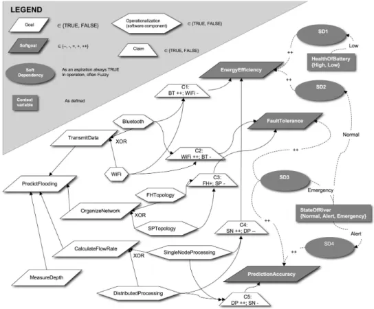
While they are not identical, features and requirements are related since features exist to satisfy requirements. It is not therefore such a big step to use requirements as proxies for features and model requirements variability instead of feature variability. Unsurprisingly, therefore, goal modeling [11] (where goals derive requirements) has also been used for modeling variability [8]. Goal modeling is particularly useful for reasoning about variants that have different QoS requirements (or softgoals). Thus (e.g.), two variants may have a common goal but offer alternative ways to operationalize the goal to achieve different levels of QoS. Figure 2 shows a simplified goal model of GridStix represented as a variant of KAOS [11]. The main elements in the models are:
• Goals, shown as white parallelograms, indicate the (functional) purpose of the system. Goals are either satisfied (TRUE) or denied (FALSE).
• Softgoals, shown as grey parallelograms, are a specific kind of goal, specifying the system’s non-functional requirements (QoS). The extent to which a softgoal is satisfied is modeled on an ordinal scale in which the set of values is {--, -, =, +, ++}, ranging from complete denial (--) through neutral or undefined (=) to complete satisfaction (++). • Goal operationalizations, shown as hexagons, specify how a goal may be satisfied. Only
one operationalization may be bound (TRUE) at any instant in time, as represented by the XOR labels.
• Claims which we model using KAOS assumptions (shown as trapeziums) indicate assumptions about operationalizations’ satisfaction of softgoals. A claim is taken as TRUE until and unless runtime monitoring shows the assumption to not hold.
• Context variables, shown as rectangles, are abstractions over a part of the system’s environment, and are monitored at runtime by sensing. Context is the combination of all context variables and the set of all contexts represents the environmental variability. • Soft dependencies, shown as grey ellipses, express required levels of softgoal
satisfaction for a particular context variable value. They are soft in the sense that it may prove impossible to satisfy them for all possible values.
Figure 2. GridStix Goal Model
Modeling the system using a goal model starts with the highest-level (e.g. business) requirements, represented as goals at the root(s) of the goal model. The goals are decomposed to form a directed acyclic graph (DAG), reflecting the hierarchy of goals of the system. Eventually, goal decomposition will reach a point where it is possible to identify how to operationalize the goals; in other words to identify the software or other components to which responsibility for the satisfaction of a leaf goal is assigned. Each identified goal operationalization has a link between it and the goal it operationalizes. A goal may have several alternative operationalizations in which case the goal acts as a variation point, with the operationalizations acting as mutually exclusive alternative features. The set of possible system configurations, as defined by the set of possible operationalizations, represents the system’s architectural variability. At variation points, a decision needs to be taken about which of the alternative goal operationalizations to select. In a conventional static SPL, this decision would be taken by the analyst at design time according to a range of criteria. In a DSPL, it may also be a run-time decision driven by the current context.
Selection among the set of possible operationalizations to be deployed is made on the basis of softgoals, for which an optimal satisfaction is sought for each context. To help achieve this, the contexts that represent environmental variation need to be identified. The impact an operationalization is believed to have on a softgoal is recorded using a claim, linked to both the operationalization and the softgoal. For each identified context, one or more soft dependencies is defined to specify the degree of satisfaction required for one of the softgoals. Thus claims and soft dependencies are orthogonal. Claims specify the QoS expected from particular operationalizations, while soft dependencies specify the QoS required under particular context variable values.
Using the set of claims and soft dependencies, for each context the set of goal operationalizations is selected that (as predicted by the claims) will come closest to achieving the required degrees of softgoal satisfaction.
In Figure 2, there are three softgoals; EnergyEfficiency, FaultTolerance and PredictionAccuracy. The single root goal is to PredictFlooding, which has been refined into a number of sub-goals. Goal refinement eventually leads to the derivation of leaf goals, such as TransmitData, for which a goal operationalization can be identified. In the GridStix case, this means a software component or configuration of components can be identified that satisfies the goal. TransmitData can be operationalized using either a Bluetooth or a WiFi component.
In Figure 2, claim C1 indicates that using Bluetooth has a strongly positive (++) effect on EnergyEfficiency, while WiFi has a weakly negative (-) impact. Thus, a configuration that uses the BlueTooth component is likely to satisfy the EnergyEfficiency softgoal better than WiFi. This advantage is reversed for FaultTolerance where BlueTooth’s low power consumption results in a comparatively short range, worsening the risk of network fragmentation.
Claims represent assumptions and reflect the fact that sometimes, the way we operationalize a goal does not result in the anticipated QoS levels. In GridStix, for example, achievement of expected QoS is subject to the uncertainties characteristic of WSNs. For this reason, claims are monitored at run-time in order to check their validity. Claim monitoring is a complex issue that we do not have space to examine here (see [12]) beyond noting that in the worst case, evaluating the truth or falsity of a claim may require the statistical interpretation of empirical data collected over prolonged periods. The key point is that claims may be subject to revision at run-time. Because a claim informs decisions taken at design time, revision of the claim caused by the accretion of empirical evidence for how an operationalization really satisfies a softgoal, means that the decisions will need to be retaken, possibly at runtime and using automated reasoning.
Context in Figure 2 comprises the two context variables: StateOfRiver and HealthOfBattery. Domain analysis indicates that the state of the river can be; normal (the river is quiescent), alert (flow rate has increased, but not depth) or emergency (flood). Battery health is modeled using only two states; low and high. GridStix’ context can therefore be represented as a set of 6 possible value pairs, representing StateOfRiver and HealthOfBattery. In Figure 2, SD1 is an example of a soft dependency and specifies that when the health of the battery is low, GridStix’s EnergyEfficiency should be at its highest (++).
Model Reasoning
Figure 2 illustrates how it is possible to treat a self-adaptive system as a DSPL, and use goal modeling to represent architectural and environmental variability, and to reason about the extent to which different variants (component configurations) satisfy the soft constraints. Even in a model as small as that in Figure 2, it may be difficult to use the set of claims to derive a variant for each context that satisfies the soft dependencies. In complex systems there may be thousands of possible component configurations [4] and many soft dependencies, leading to a risk of defining ones that are mutually inconsistent, contradictory, or simply unachievable. Thus a systematic or automatic means for analyzing a DSPL, exposing inconsistencies and deriving the set of valid variants for any context is needed.
1. At design time domain, a goal model of the DSPL is constructed, as described in the previous section, and verified to avoid defects of the types described above. Once verified, a variant is sought for each context that best satisfies the soft dependencies, even if none exists that can satisfy them all. To achieve this, we transform the goal model into a Constraint Program (CP) that can be executed by VariaMos [6]. The transformation follows a set of mapping rules where goals, softgoals, operationalizations and context variables are modeled as variables within the CP, while claims and soft constraints are modeled as constraints within the constraint program. The CP can also represent SPL properties such as operationalization incompatibilities (excludes relationships) that cannot be easily represented in goal models.
2. Once deployed, the DSPL operates an execute, monitor, evaluate, adapt control loop. Our focus in this paper is only on the decision-making evaluate element that takes the result of monitoring as input and triggers adaptations as output. The other elements can be
provided by:
I. an adaptive architecture such as that provided by the OpenCom component model [1] and GridKit middleware [3], or by the MADAM middleware [4];
II. a means to monitor claims, by collecting data about the system and its environment and interpreting it in terms of whether it supports or refutes the claims [12].
Constraint Modeling
A constraint is a logical relationship among several unknowns (or variables), each one taking a value in a given domain of possible values, where a domain is a set of possible values that a variable can take. Constraint programming is a programming paradigm in which constraints between variables are defined declaratively and a solution is found using a solver. A constraint program is defined as a triple (X, D, C), where X is a set of variables, D is a set of domains and C is a set of constraints restricting the values that the variables can simultaneously take. Classical constraint programming deals with finite domains for the variables, which are usually mapped to ordinal values such as integers. The impact on a softgoal of a particular operationalization is represented in the constraint program by integers in the range from 0 (--) to 4 (++). Elements that take Boolean values (See Figure 2) are represented as the integers 0 and 1.
Solving constraints involves first reducing the variable domains by propagation techniques [9] that will eliminate inconsistent values within domains, and then finding values for each constrained variable in a labeling phase. The labeling phase iteratively grounds (i.e. fixes a value to) each variable and propagates its effect onto other variable domains by again applying the same propagation technique. The net effect of this is to make verification and evaluation of the transformed goal model very efficient by using optimization techniques proven for solving hard combinatorial problems.
To illustrate the derivation of a constraint program, the GridStix goal model in Figure 2 can be transformed as follows:
• The group cardinality dependency between the goal TransmitData and the software components Bluetooth and WiFi is represented by the following constraint:
Which means that if TransmitData is satisfied (equal to 1), then exactly one of Bluetooth and WiFi must be satisfied too, and vice versa.
• The claims are reified as variables that can be satisfied or not by the user as an input value. For instance, in the claim C1, the value 4 means that Bluetooth fully satisfies (++) EnergyEfficiency. WiFi weakly impedes (-) EnergyEfficiency so has the value 1. This is represented by:
C1 ! (Bluetooth " EnergyEfficiency = 4) ! (WiFi " EnergyEfficiency = 1).
• The soft dependencies are reified as Boolean variables. For instance, SD1 specifies that if the health of the battery is low then EnergyEfficiency should be fully satisfied and is represented by:
SD1 ! (HealthOfBattery = 0 " EnergyEfficiency = 4).
Once the goal model is transformed into a constraint program, it can be augmented to represent properties that are hard to represent in a goal model but easy in a constraint program. For example, Bluetooth’s bandwidth is too low to support distributed processing, so the Bluetooth and DistributedProcessing operationalizations should not be used in the same variant. This can be represented as an SPL excludes relationship using the constraint:
¬(Bluetooth # DistributedProcessing)
Once the model is complete, it can be verified, analyzed and simulated with different input values. An example of verification is checking for contradictory soft dependencies. For example, a soft dependency that specified that EnergyEfficiency should be ’-‘ when StateOfRiver was Normal would contradict SD1.
Evaluation seeks to identify the optimal configuration of goal operationalizations, for any given context at design time and (if claims are revised) at runtime. To do this, constraint analysis is performed for every legal configuration.
For any context, the aim is to find at least one configuration that satisfies all the soft dependencies. To illustrate what we mean, consider the following based on the GridStix goal model:
SAT represents softgoal satisfaction values: SAT ::= -- | - | = | + | ++
These map onto the ordinal values 0 to 4 so simple arithmetic operators apply. OP represents the operationalizations :
OP ::= Bluetooth | WiFi | FHTopology | SPTopology | SingleNodeProcessing | DistributedProcessing
G represents the variation point goals:
G ::= TransmitData | OrganizeNetwork | CalculateFlowRate SG represents the softgoals:
SG ::= EnergyEfficiency | FaultTolerance |
PredictionAccuracy
CXTV ::= (HealthOfBattery, High) | (HealthOfBattery, Low) | (StateOfRiver, Normal) | (StateOfRiver, Alert) | (StateOfRiver, Flood)
Let the function operationalizes define the variation point goal that an operationalization realizes.
operationalizes: OP $ G
The function softDepends returns the required level of satisfaction of a softgoal for a particular context variable value.
softDepends: CXTV X SG $ SAT
The function claim returns the predicted level of satisfaction of a softgoal by an operationalization.
claim: OP X SG $ SAT
config defines the set of operationalizations (op) that satisfy the soft dependencies for each softgoal (sg) for a given context variable value (cxtv). Note that config will not necessarily define the full set of operationalizations, since it only contains operationalizations that affect a softgoal that participates in one of the soft dependencies defined for that context variable.
config = {%cxtv:CXTV, &sg:SG|%op:OP claim(op, sg) ' softDepends(cxtv, sg) • op}
A configuration must not contain two different operationalizations of the same variation point goal because they are always XOR-ed.
&op1 ( config, ¬% op2 ( config, %g:G|
op1 ) op2 # op1 operationalizes g # op2 operationalizes g
For every combination of context variable values that represent a context, VariaMos tries to find a legal configuration. In GridStix, this means that for every HealthOfBattery, StateOfRiver pair, a configuration is sought that satisfies both the HealthOfBattery value and the StateOfRiver value. In addition, the system will use the claims to try to optimize the softgoals that do not participate in soft dependencies, and will check for excludes relations.
At design time, in the best case, for each context at least one configuration will be found that satisfies all the soft constraints. The analyst’s job then is simply to select one; typically the one that maximizes softgoal satisfaction. Thus, for example for the context (StateOfRiver, Emergency), (HealthOfBattery, High), the optimal configuration would be {WiFi, FHTopology, DistributeProcessing}. This is because WiFi and FHTopology when combined result in complete satisfaction of the FaultTolerance softgoal as specified by SD3, while DistributedProcessing maximizes satisfaction of the softgoal PredictionAccuracy.
If no variant exists that satisfies all the soft dependencies for a given context, the analyst either needs to re-think the soft dependencies, find some alternative (better) goal operationalizations or (more commonly) accept that the soft dependencies can’t all be satisfied in this context and select a configuration that satisfies as many of the soft dependencies for that context as possible. This would be the case for the context (StateOfRiver, Emergency), (HealthOfBattery, Low) where SD1 specifies that EnergyEfficiency be maximized, and SD3 specifies that FaultTolerance and PredictionAccuracy be maximized. It is impossible to satisfy both SD1 and SD3 because SD1 can only be achieved by a configuration that uses BlueTooth and
SingleNodeProcessing, while S3 needs WiFi and DistributedProcessing. Here, the analyst would need to make a judgement about which of FaultTolerance and PredictionAccuracy, and EnergyEfficiency were most important. Since, WiFi and DistributedProcessing maximize more of the softgoals this would be the default choice.
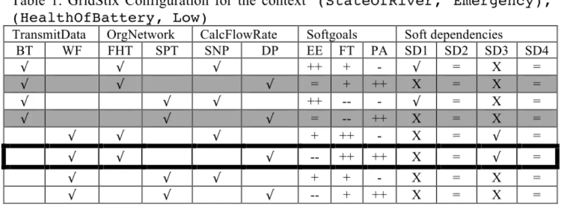
Table 1 summarizes the various configurations for the context (StateOfRiver, Emergency), (HealthOfBattery, Low). Note that a ‘=’ in a soft dependency column means simply that the soft dependency doesn’t apply in this context. The rows in grey are illegal configurations because they conflict with the constraint that BlueTooth and DistributedProcessing are mutually exclusive. The row with the bold outline is the optimal configuration since although SD1 is not satisfied, SD3 is and two softgoals are maximized.
Table 1. GridStix Configuration for the context (StateOfRiver, Emergency), (HealthOfBattery, Low)
TransmitData OrgNetwork CalcFlowRate Softgoals Soft dependencies BT WF FHT SPT SNP DP EE FT PA SD1 SD2 SD3 SD4 * * * ++ + - * = X = * * * = + ++ X = X = * * * ++ -- - * = X = * * * = -- ++ X = X = * * * + ++ - X = * = * * * -- ++ ++ X = * = * * * + + - X = X = * * * -- + ++ X = X =
Once a configuration has been defined for each context, the DSPL will adapt to the appropriate configuration whenever sensing detects a new context. However, over time, monitoring the claims may cause their revision. Monitoring can result in three things:
1. No evidence is found that the claim is incorrect;
2. The evidence shows the claim to be false but does not support computation of an accurate value. By default the effect on softgoal satisfaction predicted by the claim is automatically revised to neutral [12];
3. A new value for the claim may be computed from the collected monitoring evidence. Cases (2) and (3) constitute changes to the goal model, meaning that the DSPL’s architectural configurations may be invalid. For case (2), it would be possible to evaluate the goal model at design time to pre-compute the optimal configuration under each context using a series of what-if scenarios for refuted claims. For case (3), static evaluation isn’t practical and must be reactive to monitoring results. In this case, runtime re-evaluation is the only option so must be fully automatic.
As with the design-time computation of the per-context configurations, where no optimal configuration exists, a configuration must be sought that satisfies as many soft dependencies as possible. For example, it may turn out that DistributedProcessing does not in fact yield better prediction accuracy than SingleNodeProcessing, and claim C5 is automatically revised to (DP =; SN =) (case 2 above). Now, for the (StateOfRiver, Emergency), (HealthOfBattery, Low) context, there would be a tie between WiFi and SingleNodeProcessing and BlueTooth and SingleNodeProcessing for the optimal configuration. In fact, the former would be selected to minimize reconfiguration costs since WiFi is already the bound operationalization for TransmitData.
Where runtime recomputation of the optimal configurations is necessary (case 3 above), a performance overhead is incurred. However, in contrast to the design time evaluation, the whole model need not be evaluated at once. The optimal configurations only needs to be
found for a particular context when that context becomes current. In GridStix, only 6 (8 minus the 2 illegal combinations of Bluetooth and DistributedProcessing) configurations need to be evaluated, whereas if it had been necessary to evaluate these 6 configurations for all 6 contexts, the value would be 36. Thus, the degree of environmental variability has no impact on the cost of runtime efficiency, which is dominated by the complexity of the architectural variability.
Conclusions
Self-adaptive systems that use architectural adaptation can be conceptualized as dynamic SPLs. This is an attractive notion because work on SPLs has resulted in powerful techniques for modeling architectural variability. However, conventional SPL models cannot easily handle two important properties of DSPLs; environmental variability and QoS. Our contribution is to combine goal modeling with constraint programming. Goals support the modeling of environmental variability and QoS as well as a subset of the concepts needed for the effective representation of architectural variability. A goal model can be mapped to a constraint program, which has the added capability to represent properties such as excludes relationships that are hard to represent in goal models. Moreover, a constraint program, when solved using a tool such as VariaMos, is able to determine the extent to which the set of variants for any context meet the QoS requirements. The key advantages of our approach are that it allows the analyst to perform static verification of the goal model that captures the requirements and assumptions for a DSPL, and that the same techniques can be used to dynamically re-evaluate the goal model as assumptions are revised in the light of evidence acquired by runtime monitoring.
There are, of course limitation to our approach. Our approach would not work where a high degree of environmental complexity made it impossible to identify a discrete set of contexts
a-priori. However, we are confident of our constraint programming approach’s ability to deal
with significant architectural variability. Computation of the optimal configuration for any GridStix context takes c. 20ms on a standard PC. GridStix has relatively little architectural variability, but we have tested VariaMos on static SPLs running to many thousands of features, and including the added complexity of optional features that are absent from our WSN models. These experiments show that VariaMos evaluates these product line models in linear or polynomial time.
Generalizing the above, finding the per-context optimal architectural configuration is essentially a problem of multi-criteria decision-making (MCDM), and this is an acknowledged open problem for self-adaptive systems [7]. However, in our approach we only attempt to optimize softgoals. We treat (functional) goal satisfaction as Boolean and the set of goals and softgoals as fixed and unchanging. All that varies is:
• the required degree of softgoal satisfaction that is defined per context;
• the expected degree of softgoal satisfaction achievable by the different goal operationalizations.
Both of these are measured using a discrete set of ordinal values. The net effect is to allow our approach to exploit the highly efficient capabilities of modern constraint program solvers. Our approach still suffers the problem common to other MCDM techniques whereby the assignment of the right weights (required and estimated degrees of softgoal satisfaction in our case) can be hard. At least with our approach, claims can be revised using empirical evidence gathered by runtime monitoring.
Memory consumption may be more of an issue for WSNs but even here, with careful design and appropriate middleware support, processing can be performed off-line and new configurations (or rather the policy rules that select components) distributed to the nodes. Note that in any case this is likely to be needed only rarely, when a claim is revised. We are
therefore confident that constraint programming holds real promise for DSPLs combining significantly greater scale and complexity than GridStix, our exemplar DSPL.
References
1. Coulson, G., Blair, G., Grace, P., Joolia, A., Lee, K., Ueyama, J., Sivaharan, T. (2008) “A generic component model for building systems software”. ACM Transactions on
Computer Systems, 26 (1).
2. Hallsteinsen, S.; Hinchey, M.; Sooyong Park; Schmid, K. (2008) “Dynamic Software Product Lines” IEEE Computer, 41 (4).
3. Hughes, D., Greenwood, P., Coulson, G., Blair, G., Grace, P., Pappenberger, F., Smith, P., Beven, K. (2008) “An experiment with reflective middleware to support grid-based flood monitoring,” Concurrency and Computation: Practice and Experience, 20 (11). 4. Khan, M. U., Reichle, R., Geihs, K. (2008) “Architectural Constraints in the
Model-Driven Development of Self-Adaptive Applications”, IEEE Distributed Systems Online 9 (7)
5. Mckinley, P., Sadjadi, S., Kasten, E., Cheng, B. (2004) “Composing adaptive software” IEEE Computer 37 (7)
6. Mazo, R., Salinesi, C., Diaz, D., Djebbi, O., Lora-Michiels, A. (2012) “Constraints: the Heart of Domain and Application Engineering in the Product Lines Engineering
Strategy”, International Journal of Information System Modeling and Design (IJISMD), 3 (2).
7. Sawyer, P., Bencomo, N., Whittle, J., Letier, E., Finkelstein, A. (2010) “Requirements-aware systems: A research agenda for RE for self-adaptive systems,” 18th IEEE International Conference on Requirements Engineering (RE’10), Sydney, Australia. 8. Semmak, F., Gnaho, C., Laleau, R. (2010) “Extended KAOS Method to Model
Variability in Requirements” in (Maciaszek, L., González-Pérez, C., Jablonski, S. Eds) Evaluation of Novel Approaches to Software Engineering, Springer Berlin Heidelberg. 9. Schulte, C., Stuckey, P. (2008) “Efficient constraint propagation engines” ACM Trans.
Program. Lang. Syst. 31 (1).
10. Sykes, D., Heaven, W., Magee, J., Kramer, J. (2010) “Exploiting non-functional preferences in architectural adaptation for self-managed systems” Proc. ACM Symposium on Applied Computing (SAC '10), New York, NY.
11. van Lamsweerde, A. (2009) Requirements Engineering: From System Goals to UML Models to Software Specifications. John Wiley & Sons, Chichester, UK.
12. Welsh, K., Sawyer, P., Bencomo, N. (2011) ”Towards Requirements Aware Systems: Run-time Resolution of Design-time Assumptions”, Proc. 26th IEEE/ACM International Conference on Automated Software Engineering (ASE’11), Lawrence, Kansas.
Author Biographies
Pete Sawyer is Professor of Software Systems Engineering at Lancaster University. His
primary research interests are in requirements engineering, self-adaptive systems and knowledge management. Sawyer received a PhD in Computer Science from Lancaster University. He is a member of the IEEE, the ACM and the British Computer Society.
Raúl Mazo is an Associate Professor at Université Paris 1, Panthéon Sorbonne. His research
interests include the definition of constraint-based formalisms to represent complex product line models, the definition of methods to validate, verify, analyse, configure and evolve variability models and the construction of product line models. Mazo received a PhD in Computer Science from Université Paris 1, Panthéon Sorbonne. Contact him at:
Daniel Diaz is an Associate Professor at Université Paris 1, Panthéon Sorbonne. He is
member of the Centre de Recherche en Informatique. He is the author of GNU Prolog. His research interests include: Logic Programming, Constraint Programming, Local search and parallelism. Diaz received his PhD from Université d'Orléans. Contact him at:
Camille Salinesi is a Professor at Université Paris 1, Panthéon Sorbonne. He is the head of
the Centre de Recherche en Informatique, which specializes in Information Systems
Engineering. His research interests include requirements engineering, strategic alignment and product lines. Salinesi received a PhD from Université Paris 6, Pierre et Marie Curie. Contact him at: [email protected]
Danny Hughes is an Assistant Professor with the IBBT-DistriNet research group of KU
Leuven. His research interests focus on reconfigurable component models, service oriented architectures and self-adaptive middleware for networked embedded systems. Hughes received a PhD in Computer Science from Lancaster University. He is a member of the IEEE and the ACM. Contact him at: [email protected]
Contact Information:
Pete Sawyer: School of Computing and Communications, InfoLab21, Lancaster University,
Lancaster, UK. LA1 4WA. +44 1524 510320, [email protected]
Raul Mazo: Centre de Recherche en Informatique (CRI), Université Paris 1 Panthéon
Sorbonne, 90 rue de Tolbiac, 75013 Paris, France. +33 1 44 07 86 45, [email protected]
Daniel Diaz: Centre de Recherche en Informatique (CRI), Université Paris 1 Panthéon
Sorbonne, 90 rue de Tolbiac, 75013 Paris, France. +33 1 44 07 89 61, [email protected]
Camille Salinesi: Centre de Recherche en Informatique (CRI), Université Paris 1 Panthéon
Sorbonne, 90 rue de Tolbiac, 75013 Paris, France. +33 1 44 07 86 45, [email protected]
Danny Hughes: IBBT-DistriNet, Department of Computer Science, KU Leuven,
Celestijnenlaan 200a, B-3001 Heverlee, Belgium. + 32 16 3 28287, [email protected]