Computational design and optimization of infrastructure policy in water and agriculture

Computational Design and Optimization of

Infrastructure Policy in Water and Agriculture

by

Abdulaziz Alhassan

B.S., King Fahd University of Petroleum and Minerals (2013)

Submitted to the Center for Computational Engineering

in partial fulfillment of the requirements for the degree of

Masters of Science in Computation for Design and Optimization

at the

MASSACHUSETTS INSTITUTE OF TECHNOLOGY

June 2017

@

Massachusetts Institute of Technology 2017.

Author...

Certified by....

a

All rights reserved.

A N

Signature redacted

- -% '.

Center for ,4omputational Engineering

Signature redacted

M

_ay

t/11-

-24, 2017

Olivier L. de Weck

Professor of Aeron

ics and stro utics and Engineering Systems

A17/

7 V

rThesis

_Supervisor

Certified by.

Signature redacted

....

Kenneth Strzepek

Research Scientist, Joint Pg

3ra

and CGCS. Professor Emeritus of

Civil, Environmental, and Architectural Engineering, University of

Boulder at Colorado

Accepted by ..

MASSACHUSETS INSTITUTE

OF TECHNOLOGY

JUN 19 2017

Signature

redactedhesis

Supervisor

...

icolas Hadjiconstantinou

Co-Director, Computation

r Design and Optimization

I

Computational Design and Optimization of Infrastructure

Policy in Water and Agriculture

by

Abdulaziz Alhassan

Submitted to the Center for Computational Engineering on May 24, 2017, in partial fulfillment of the

requirements for the degree of

Masters of Science in Computation for Design and Optimization

Abstract

Investments in infrastructure tend to be associated with high capital costs, creating a necessity for tools to prioritize and evaluate different infrastructure investment op-tions. This thesis provides a survey of computational tools, and their applicability in fine-tuning infrastructure policy levers, prioritizing among different infrastructure investment options and finding optimal sizing parameters to achieve a certain ob-jective. First, we explore the usability of Monti Carlo simulations to project future water demand in Saudi Arabia and then, we use the outcome as an input to a Mixed Integer Linear Program (MILP) that investigates the feasibility of seawater desali-nation for agricultural irrigation under different water costing schemes. Further, we use numerical simulations of partial differential equations to study the conflicting interests between agricultural and municipal water demands in groundwater aquifer withdrawals and lastly we evaluate the use of Photo Voltaic powered Electro Dialy-sis Reversal (PV-EDR) as a potential technology to desalinate brackish groundwater through a multidisciplinary system design and optimization approach.

Thesis Supervisor: Olivier L. de Weck

Title: Professor of Aeronautics and Astronautics and Engineering Systems Thesis Supervisor: Kenneth Strzepek

Title: Research Scientist, Joint Program and CGCS. Professor Emeritus of Civil, Environmental, and Architectural Engineering, University of Boulder at Colorado

Acknowledgments

To my parents, Abdulrahman and Hessa, for their utmost care and encouragement, for always placing their faith in me and pushing me through my endeavors. To my siblings, Mohammed, Riyadh, Faten, Rami, Ziyad, Areej and Ahmed for always being there for me.

To my friends, for providing a network of guidance and companionship when needed the most. My teachers, mentors and professors, to their passion, knowledge and wisdom that enabled me to grow.

To my advisors, Olivier de Weck, who have always provided a unique point of view, and Kenneth Strzepek, a passionate water scientist on a long journey around the world to solve problems and raise awareness, who took me under his wings and made sure I had what it takes to be a better informed water person.

To MIT, and the Center for Computational Engineering, for providing an envi-ronment for innovation to thrive. To King Abdulaziz City for Science and Technology for paving my way forward and for their generous scholarship that made this possible. To the Center for Complex Engineering Systems and its co-director, Anas Alfaris for pushing me to the limit.

Contents

1 Introduction

1.1 M ain Contribution . . . .

1.2 Planning, Policymaking, and Reforms in Saudi Arabia . . . .

2 Modeling Saudi Arabia's Water Resources

2.1 Water Resources in Saudi Arabia . . . .

2.2 Overview of Water Supply and Demand In Saudi Arabia . . . .

2.3 Demand Projection Methodology . . . .

2.4 Municipal Water Demand . . . .

2.4.1 Background . . . .

2.4.2 Municipal Demand Projections . . . .

2.5 Agricultural Water Demand . . . .

2.5.1 Background . . . .

2.5.2 Agricultural Water Demand Projection . . . .

2.6 Water Supplies in Saudi Arabia . . . .

2.7 C onclusion . . . .

3 Saudi Arabia's Agriculture Policy

3.1 Background . . . .

3.1.1 Economic Implications of Agriculture . . . .

3.1.2 Food Im ports . . . .

3.2 Spatial Distribution of Agricultural Groundwater Withdrawals

3.3 The Energy Footprint for Water in Agriculture . . . .

17 17 19 21 21 23 24 25 25 28 32 32 32 34 38 39 . . . . 39 . . . . 40 41 . . . . 44 . . . . 45

3.4 The Potential of Seawater Desalination for Agriculture . . . .

3.5 W ater Pricing . . . .

3.5.1 The Cost of Virtual Water Imports . . . .

3.5.2 The Cost of Groundwater Pumping and the willingness to Pump

3.5.3 The Cost of Desalination and the Willingness to Desalinate . .

3.5.4 Comparison to Current Tariffs . . . .

3.6 C onclusion . . . .

4 Simulating Water Competition Between Municipal and Agricultural Uses in Riyadh 4.1 4.2 4.3 4.4 4.5 4.6 4.7 Background . . . . Simulation Scope . . . . Governing Equations . . 4.3.1 Groundwater flow Methodology . . . . Accuracy Estimation . . Results . . . . Conclusions . . . . equation 47 51 51 51 52 52 52 55 55 55 58 58 59 63 63 67 5 Cost-Optimizing Photovoltaic Powered Electrodialysis

EDR) Systems for Off-Grid Settings

5.1 Introduction . . . . 5.1.1 Background . . . . 5.1.2 EDRvs. RO . . . . 5.1.3 PV Power Source . . . . 5.2 System Model . . . . 5.2.1 Overview . . . .

5.2.2 Optimization Problem Formulation . . . .

5.2.3 Single-Objective Optimization Algorithms . . .

5.2.4 Multi-Objective Optimization . . . .

5.3 Results and Discussion . . . .

Reversal (PV-69 . . . . 69 . . . . 70 . . . . 71 . . . . 73 . . . . 73 . . . . 73 . . . . 77 . . . . 79 . . . . 81 82

5.3.1 Single-Objective Optimization Results . . . . 82

5.3.2 Multiple-Objective Optimization Results . . . . 82

5.3.3 Sensitivity Analysis . . . . 82

List of Figures

2-1 Historical Agricultural, Industrial and Municipal water demand [2] . 23

2-2 Historical desalination contribution to municipal demand, by region [9] 27

2-3 Historical municipal demand per capita [91 . . . . 27

2-4 Historical municipal water demand showing seasonality and

contribu-tion of groundwater and desalinacontribu-tion, nacontribu-tional [9] . . . . 28

2-5 Three scenarios for per capita water demand projections . . . . 29

2-6 Three scenarios for Population projections . . . . 30

2-7 Three scenarios for municipal water demand projections, obtained by

using population as a driver, and per capita water consumption as an

indicator . . . . 31

2-8 Three scenarios for Crop land areas across the four crop families . . . 33

2-9 Three scenarios for agricultural water demand projections, obtained by

using crop family land area as a driver, and per area water requirement

as an indicator . . . . 35

2-10 Supply requirements of the 27 scenario combinations . . . . 37

3-1 Historical agricultural land area showing major crop families, national

[10] . . . . 40 3-2 Agricultural GDP, and contribution of agriculture to overall GDP,

na-tional [101 . . . . 41 3-3 Comparing 10 economic sectors of the economy in terms of GDP and

3-4 Comparing 10 economic sectors of the economy in terms of

Employ-ment and Labor Compensation . . . . 42

3-5 Saudi Arabia's local production of food, and food imports [18] . . . . 43 3-6 Estimates of Saudi Arabia's virtual water imports, and the price per

cubic meter of virtual water imported. . . . . 43

3-7 Cumulative agricultural water withdrawals across 13 regions between

1999 and 2013 . . . . 45

3-8 Spatial distribution of groundwater withdrawals . . . . 46

3-9 Energy Intensity of Agricultural Water Withdrawals . . . . 47

3-10 27 agricultural zones, municipal demand nodes and the existing

desali-nation network . . . . 49

3-11 The optimized agriculture desalination network at 2050 . . . . 50 3-12 The cost of using Photo Voltaic Multi Effect Destination (PV-MED)

on the coast of the Red Sea . . . . 53

3-13 Comparing old, new water tariffs to four proposed water pricing metrics 54 4-1 The location of eight well fields supplying Riyadh, Saudi Arabia is

shown by the eight circles, the city is shown by the blue square, and

the analyzed three agricultural clusters are shown as black diamonds. 57

4-2 Historical daily water withdrawals from the eight well fields . . . . 57

4-3 Visualizing the A matrix resulting form a central difference discretization 62

4-4 The result of running a grid refinement study to the finite differences

schem e . . . . 64

4-5 Results of the simulation showing the water level for the current

situ-ation, full agricultural activity and municipal water demand. . . . . . 65

4-6 Results of the simulation showing the water level for the proposed

scenario of limiting agricultural activity and only keeping municipal

water dem and. . . . . 66

4-7 The difference between the two simulations, this figure shows the drop

4-8 The national agricultural system, the elements studied in this analysis

appear in the central region, and they only constitute a small fraction

of the national system .. . . . . 68

5-1 Reverse osmosis. [28] . . . . 71

5-2 Electrodialysis. [28] . . . . 72

5-3 Graphical depiction of the PV power system model. The parabolic

curve is the PV power output over the course of a day. The rectangular

curve is the EDR power requirement. The shaded area represents the

required energy storage capacity for this design configuration. .... 76

5-4 Steepest descent solution traces. . . . . 79

5-5 Pareto front generated by the manual weighted sum. . . . . 83

5-6 Sensitivity analysis of the PV-EDR system to changes in intake salinity

List of Tables

2.1 Variations of population, growth, demand and per capita municipal

dem and [2, 81 . . . . 26

3.1 Desalination for agriculture; Capital costs, operational costs and C02 emissions resulting form the INFINIT simulation run. . . . . 48

4.1 A list of the eight municipal water wells, and the three agricultural zones, and their corresponding annual water withdrawals . . . . 56

5.1 PV Subsystem Parameters . . . . 78

5.2 EDR Subsystem Parameters . . . . 78

5.3 Cost and Replacement Frequency Parameters . . . . 78

5.4 PSO Tuning Parameters . . . . 81

Chapter 1

Introduction

1.1

Main Contribution

Investments in infrastructure tend to be associated with high capital costs, creating

a necessity for tools to prioritize and evaluate different infrastructure investment

options, such as technology use and sizing. While numerical simulations provide

a tool to analyze and understand the environment that infrastructure operate in, such as simulating seawater salinity, groundwater flow, storms and dust patterns.

Optimization provides a decision tool that could help infrastructure policymakers to

investigate many alternatives such as the optimal economic benefit of agriculture, optimal water allocation between competing activities, selecting optimal sizing and

technology choice of an infrastructure plant.

This thesis provides a survey of a number of computational tools, and their

ap-plicability in fine-tuning infrastructure policy levers, prioritizing among different in-frastructure investment options and finding optimal sizing parameters to achieve a

certain objective.

The Second Chapter assesses the water balance in Saudi Arabia, and explores the usability of Monti Carlo simulations to project future water demand in Saudi Arabia on a regional level for both municipal demand and agricultural demand. For each demand category, three demand scenarios are picked as expected high, medium and

source composition.

The Third Chapter starts off with an investigation of agricultural economics and history in Saudi Arabia, and looks at the food balance in the country. A spatial representation of agriculture in the country is constructed. That spacial representa-tion together with the agricultural demand forecasts constructed in Chapter Two are used as inputs to a Mixed Integer Linear Program (MILP), an optimization tool that investigate the feasibility of seawater desalination for agricultural irrigation. Later, a set of alternative water pricing schemes are constructed that are driven by willingness to pump groundwater, willingness to desalinate seawater and the cost of virtual water imports. Those water pricing schemes are compared to the current municipal water tariff in Saudi Arabia.

In Chapter Four, a numerical simulation of the groundwater partial differential equation is developed, using a finite difference scheme to study the conflicting inter-ests between agricultural and municipal water demands in groundwater aquifer with-drawals around the city of Riyadh, Saudi Arabia. The accuracy of that simulation is analyzed, and then provide an assumption biased quantification of the hydraulic head change with and without agricultural activity around the city.

Chapter Five analyzes the use of Photo Voltaic powered Electro Dialysis Reversal (PV-EDR) as a potential technology to desalinate brackish groundwater for munici-pal use in Saudi Arabia through a multidisciplinary system design and optimization approach. The chapter begins by defining a model and its submodules, and then constructing a set of objective functions. A full factorial design space exploration is used, and then optimal solutions are found through gradient based and heuris-tic based methods. multiple objectives are handled through a manual weighted sum method and a full factorial study. Outcomes are compared in both the gradient-based optimization and the heuristic based optimization.

1.2

Planning, Policymaking, and Reforms in Saudi

Arabia

Saudi Arabia issued it's first "Development Plan" in 1970. That plan aimed to achieve economic diversification away from oil exportation as its first priority. The 10th Plan was released in 2015 and had similar goals to the first few ones. Particularly, the diversification goal was in every development plan ever issued in the 45 years between

1970 and 2015, but the government's income base has been dominated by oil rents.

The collapse of oil prices in the end of 2014, and the sustained low prices that followed, prompted the government to exercise many austerity measures: including reductions in capital investments, freeze in government workers raises and slashes in benefits, phasing out many government subsidies in the water and energy sectors, and (for the first time in its history) imposing a value added tax (VAT). Those policy reforms were rolled out as part of the Fiscal Balance Program announced in 2016, which aims to eliminate government deficit that resulted from the 2014 decline in oil prices. This Fiscal Balance Program is one of a set of programs under the "Vision 2030", an overarching framework meaning to achieve the historic goal of weaning the Saudi Arabian economy away from dependence on oil rents, with minimal socioeconomic disruption.

New policy reforms under "Vision 2030" share a few basic objectives: spending rationalization, efficiency increases and subsidy cuts. one can argue that the analysis provided in this thesis can provide a starting point for a policy-driven, optimality ori-ented, efficient water infrastructure planning toolkit. This work is intended to serve as a survey for a set of tools and their applicability to decision making and infrastruc-ture policy agenda setting. The conclusions discussed henceforth are dependent on the specific spatio-temporal context and should only be taken as a pre-feasibility anal-ysis. Further, location specific, context specific analysis is needed to enable decision making on a refined level.

Chapter 2

Modeling Saudi Arabia's Water

Resources

2.1

Water Resources in Saudi Arabia

Saudi Arabia, although energy rich, is poor in its water resources. The country is part of an arid region where there is no access to any form of fresh surface water. Saudi Arabia resorted to the energy intensive seawater desalination for municipal use to supplement groundwater resources that are being strained by agricultural activ-ity, raising the need to study the country's water-energy-food nexus. This chapter uses population and agricultural trends to build futuristic water demand scenarios, and proposes a set of variations on population growth and agricultural policy. This chapter matches demand scenarios with supply scenarios. Exploring the effect of these variations, estimates the possible ranges of resources needed, either as ground-water withdrawals or as energy requirements for desalination. This enables decision makers to make better-informed sustainable decisions. A specific policy on seawater desalination for agriculture is thoroughly investigated.

Saudi Arabia is divided into 13 administrative regions; each region has a capital that is usually the largest city in that region. In 2010, the population of Saudi Arabia was 27 million, 65% of the population lived in the three major regions of Saudi Arabia: Makkah, Riyadh and the Eastern Region [1]. This chapter will look into the water

balance of Saudi Arabia on the regional level.

The scarcity of rainfall in Saudi Arabia led to the absence of any permanent sources of surface water, forcing Saudi Arabia to rely on two main sources to satisfy water demand: ground water aquifers and seawater desalination. Presently, agricultural demand depends completely on ground water, while industrial and municipal demand are met through a combination of groundwater extraction and seawater desalination

[2].

Groundwater in Saudi Arabia can be described as fossil water. Due to limited rainfall and excessive consumption, the major groundwater aquifers are being de-pleted. A study estimated the storage of the main and secondary aquifers in 1984 to be around 500 billion cubic meters and a study in 1996 estimated the amount to be

289.1 billion cubic meters [4]. Taking into consideration the reported consumption

rates since then, the state of groundwater resources in Saudi Arabia is unsustainable

[5], and measures should be taken from either demand or supply side (or both) to put

the state of water resources in a more sustainable path.

The state of the groundwater is based on limited available data with a large degree of uncertainty. This is due to the fact that estimating exact figures of ground water levels is a difficult and uncertain task. We could end up either overestimating or underestimating ground water levels with a significant margin of error. More studies are needed to better evaluate the current state of ground water levels to make plans that are more reliable for the future. In addition, it is unclear if we are constrained

by extraction rates. It's uncertain that Saudi Arabia could reach a point in which

possible extraction rates could be a limiting factor to supply.

Excessive extraction of groundwater is associated with increased financial costs. Lower groundwater levels would add more energy demand for extraction from deeper wells. Deeper wells cost more to be dug, and water quality degrades significantly with excessive groundwater withdrawal [4, 6].

This study proposes regional scenarios where alternatives in major demand drivers are used, and matched with proposed supply scenarios, The scenarios are applied to Saudi Arabia as a case study.

20000 National Water Demand in Saudi Arabia 15000 10000 U C 5000 2874 Munidpal OM _____________________________~

~~~~~~~~~~

9_________________________________ 30 minuscal Daa 2&5 2006 2007 2008 2009 2010 2011 2012 2013 2014 Years

Figure 2-1: Historical Agricultural, Industrial and Municipal water demand [2]

2.2

Overview of Water Supply and Demand In Saudi

Arabia

We can see from Figure 2-1 that agricultural water demand constitutes 83% of the total water demand in Saudi Arabia in 2014. The remaining 17% is municipal and industrial water demand

[2].

Agricultural water supplies are coming from the fossil ground water reserves. The only water costs that farmers bare is the cost of energy needed to pump water from the ground up, and they usually rely on energy resources that are heavily subsidized by the Saudi government [5]. This makes water costs marginal and there is no incentive for farmers to invest in water efficient irrigation systems.

Municipal water demand is dependent on seawater desalination (Figure 2-2). Fifty-six percent of municipal water supplies come from desalination plants that are located on both the east and west coasts of Saudi Arabia [2]. Desalinating seawater is an energy intensive process. The energy requirements of those desalination plants are supplied from Saudi Arabia's oil and gas reserves, and utility companies purchases of fuel are heavily subsidized.

2.3

Demand Projection Methodology

To project demand, a driver-intensity approach is used, where different demand

cate-gories are associated with drivers (Population, agricultural land ares,...) and

intensi-ties (Per capita consumption, crop water requirements, ... ). A Monte Carlo process is

used to project the future values of those drivers and indicators with a confidence

in-terval, and then the value of a driver is multiplied by the value of an indicator to come

up with an estimate projection for future water demand across different categories.

The Monte Carlo process looks at historical values of either a driver or an indicator, then it builds a probability distribution of historical growth rate percentages. Then

the process generates a number of random walks that draw from the constructed

random distribution. The 90th percentile, mean and the 10th percentile for those

random walks are used as the high, medium and low scenarios respectively. The

random walk is constrained by a growth rate limit, and has a diminishing factor

that declines with time. This Monte Carlo process is parameterized by the following

parameters;

" Last simulation year

" Number of random walks

* Bound on growth rates

" The diminishing factor

And the demand projection is obtained through the following formula:

MY = (1 + U(min(Dg), max(Dg)))Dy_1(1 + U(min(Ig), max(Ig)))Iy-I

Where:

" Mt': is demand projection at year y

o I Intensity value at year y

* U(min(D,), max(D,)): a random variable drawn from a uniform distribution

bounded by the minimum and maximum historical driver growth rate

Using this formula to generate multiple random walks that project future demand through indicators and drivers, we define three demand projections:

" High the ninetieth percentile of all generated demand random walks " Medium the mean of all generated demand random walks

" Low the tenth percentile of all generated demand random walks

2.4

Municipal Water Demand

2.4.1

Background

Municipal water demand in Saudi Arabia is driven by population growth. Population in Saudi Arabia grew significantly in the 1970's and 1980's with growth rates touching

6.5% due to the jump of quality of life that was associated with the government's oil

income. The period of the 1990's and the 2000's exhibited a slower population growth rates with a growth rate of around 2% in 2013 [7].

The last two official censuses (2004, 2010) show varying growth rates across re-gions. This can be attributed to the fact that some regions are more economically mature than others; causing inter-regional migration towards the more economically developed regions.

Table 2.1 shows the variation of population demand across regions. Regions vary in their water supply source. Desalination constituted 58.4% of municipal water supplies. Ninety-nine percent of municipal water supplies in Makkah region came from seawater desalination, where Hail, Northern Borders, Najran, Baha and Jawf regions relied completely on groundwater. Table 2.1 shows variation of the contribution of desalination across all regions. We can see from Figure 2-2 that the contribution of desalination is following an increasing trend.

Table 2.1: Variations of population, growth, demand and per capita municipal

de-mand [2, 8]

Popula- Munici- Munici- Per Piopa p - pal Contri- Capita Popula- Growth Demand Demand bution of consump-Region tion Rate (2013 Growth Desalina- tion

(2013) (2004 MCM Rate tion (2013,

(20104 MM Y(2006- (2013, %) M3 per

-2010) _{per Year) 2013) Person)}

Saudi 30387506 3.3 2731 5.7 58 90 Arabia Riyadh 7733415 3.9 808 4.6 41 105 Makkah 7736211 3.3 676 9.7 99 87 Madinah 1972818 3.0 178 4.6 85 90 Qassim 1360856 3.3 120 0.7 3 88 Eastern 4645516 _{3.7 599 2.9 55} 129 Region Asir 2083276 2.4 76 8.2 89 36 Tabuk 865861 2.5 99 12.2 10 114 Hail 650172 2.4 32 3.5 0 50 Northern 350702 _{2.5 23 15.7} 0 65 Borders Jazan 1496944 2.6 38 14.5 65 26 Najran 567288 3.4 24 14.5 0 42 Baha 439697 1.7 16 14.4 0 37 Jawf 496401 3.6 40 2.6 0 81

Per capita demand is also varying across regions. Figure 2-3 shows that the

Eastern Region is the highest with 129 cubic meter per person per year in 2013, while

Jazan's per capita consumption was the lowest at 26 cubic meter per capita per year.

Municipal demand can be characterized to be seasonally fluctuating, demand rises

during summer months, and maximal monthly demand usually falls around July.

Demand falls during winter, reaching minimal monthly demand around February.

Figure 2-4 shows seasonality. The proportion of maximum monthly demand to

mini-mum monthly demand averaged 1.243:1 and the fluctuation of demand is mapped to

fluctuation in both supply sources. The proportion of maximum monthly supply to

100 Desalination Contribution 80[ 60 40 20 A57 2008 2009 2010 2011 2012 2013 2014 Years

Figure 2-2: Historical desalination contribution to municipal demand, by region [9]

Per Capita Water Demand

350 300 250 200-150 100 50-207 2008 2009 2010 Years

Figure 2-3: Historical municipal demand per capita [9]

v 92 Madinah 67 jazan 38 Saudi Arab. 55 Eastem R6gion 43 Riyadh 26 Baha 10 Tab -Qaswam 6. 0 5 Gordam %74 Eastern R"an 24X Inah 170 MW 142 =:wn Owder 153 q' , -66 Nalran 76 jazan 2011 2012 2013 2014

MONTHLY WATER DEMAND - SAUDI ARABIA

250 200 / / A.// / / ./ 150 50

A'

/ 92 / / 17 N N N N 0 00 00 0 0 0 0 0 4 N N ' m GWTotal a DTotal

Figure 2-4: Historical municipal water demand showing seasonality and contribution of groundwater and desalination, national [9]

desalinated water supply respectively [9].

2.4.2

Municipal Demand Projections

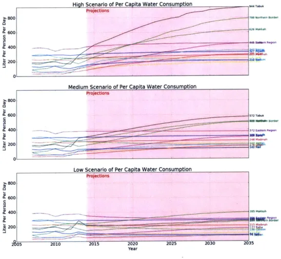
Following the earlier described Monte Carlo demand projection methodology, munici-pal demand is associated with population as a driver, and with per capita consumption as an intensity. A Monte Carlo process is used for each of the thirteen regions, for both the driver and intensities. Figure 2-5 shows three scenarios for per capita con-sumption, and Figure 2-6 shows three scenarios for population. A municipal water demand projection is then generated (Figure 2-7). The latest available data year shows that municipal demand across Saudi Arabia stands at 2,874 MCM in 2014. The high, medium and low scenarios project municipal demand to reach 5,000; 6,500;

8,000 MCM respectively of municipal demand in Saudi Arabia in 2035.

PI-1-High Scenario of Per Capita Water Consumption 9,au Projections 780 Nort~" 8~,d. 62- Makkah 45 WOM R*Won - f S s72 Tabuk Of I b Sc~ 31 InternRegio 01

Low Scenario of Per Capita Water Consumption

Projections

200z1 Uo 3

2020

Year

Figure 2-5: Three scenarios for per capita water demand projections

) 800 600 400 CL ,0200 0 600 .400 200

Medium Scenario of Per Capita Water Consumption

Projections >. 800 A600

a

400 200 2005 215Madina 39 *aka I 2025 ZUJU .9W.2. 2010 2015

Projections 2

1

2OS 2010 Projections - -Isom

MedIum Scenario of P nulto

Low Scenario of Population

Ikkah

,yadh

Year

Figure 2-6: Three scenarios for Population projections

1e7 ih ceaiofPoatn 5 4 2 1 0 5 3 2 1 0 5 4 1.7 P _{! I}

High Scenario of Population

107

e7

'1 - Medu Scnari of opulti,

Projections w

-- kkah

yadh

eom pm

q-High Scenario of Municipal Water Demand

Projections

- -

i-MediIum Scenarf of dineniWirf~~

Projections leg 7 -6 U5 2 C to E 3 0 02 2?i05 20 10

Low Scenario of Municipal Water Demand Projections

Figure 2-7: Three scenarios for municipal water demand projections, obtained by using population as a driver, and per capita water consumption as an indicator

-1eg9 7 E 3 1 0 7 -6 U ₅ 4 E 3 02 1 0 iyadh RRpM O-nt&kaon y~a Year

ea~" CgnrnMUnr lWti amn

a

I

2.5

Agricultural Water Demand

2.5.1

Background

Agricultural water demand in Saudi Arabia is investigated as it historically consti-tuted the largest bulk of national water demand. in order to build projections, the same driver-intensity approach is followed, where agricultural land areas are used as drivers, and per unit of area water requirements as intensities. As those intensities vary across geographical locations and types of crops, The analysis is broken down into four families of crops:

" Vegetables: tomatoes, cucumbers, ... etc.

* Cereals: wheat, malt, ... etc.

" Fruits: Dates, grapes, ... etc.

" Fodder: Barley, alfalfa, ... etc.

The intensities (per area water requirements) used in this analysis are based off of the ones generated in [161

2.5.2

Agricultural Water Demand Projection

From Figure 2-8, the following is observed about each of the four crop families

" Vegetables: In the near history, vegetable growing in Saudi Arabia has been

stable, as it wasn't directly impacted by a policy control. The High scenario shows a slight increase in land areas dedicated to vegetable growing, while the Medium and Low scenarios showed a slow, minor, gradual decline in areas dedicated to grow vegetables.

" Cereals: as a result of a recent policy changes (Discussed in details in

Chap-ter 3), and due to the recent inclination to import cereals as opposed to growing them locally in Saudi Arabia, we see a steady decline in the area dedicated to

Medium Scenarlo of Area ofVegitables

Low Scenario of Area of Veoltables

PrMjeto-(a) Projections of Areas of Vegetables

High Scenrlio ofArea of Fruits ____

250000

Medium Scenario of Area of Fruits

230000

-0000

LOW Scenario of Area of fruits

imp

500ooo

(c) Projections of Areas of Fruits

(b) Projections of Areas of Cereals

High Scenario of Area of Fodder

40000 asocco~

~ ~ ~

--- -.vm M200000ai f re fFoce 400000 350M 300000 "0000 nom 1100 400M 310M 300000 nom 10ow sow

(d) Projections of Areas of Fodder Figure 2-8: Three scenarios for Crop land areas across the four crop families

IZOOD 10000 .000 2000 70004 50001 40001 2000c 70004 60001 70004 f-50001 -o ---en or -re .g r-e 20-M0

growing cereals across the three scenarios, with the High scenario exhibiting a

slow decline, while the Medium and Low showing a steady and sharp declines

respectively.

* Fruits: Similar to the dynamics in vegetables, the land dedicated to grow fruits

is expected to grow in the High and Medium scenarios, while the low scenario

showed a minor decline.

" Fodder: it is interesting to observe that the area dedicated to grow fodder has

increased across the three scenarios. This can be attributed to a recent change

in policy (more details in Chapter 3), where a restriction on growing wheat

led farmers to grow fodder instead, as it uses the same infrastructure, while

it constitute an economically vital crop to farmers, and a good substitute for

the no longer subsidized wheat. While the Low scenario showed only a slight

increase, the Medium and High scenarios showed an increase of around 50%

and 100% in Fodder land areas respectively.

Using those projections in land areas dedicated to different families of crops as

drivers to agricultural water demand, and using the geographically varying crop

fam-ily water requirements generated in [16] as intensities, three demand projections are

constructed. Shown in Figure 2-9, the high scenario proposes a doubling in

agri-cultural water demand by 2035 from its levels in 2013, while the Medium scenario

projects an increase of 50% and the low scenario expects a minor increase. The

vari-ation between the three scenarios is mainly a result of the varivari-ation of the amount

of land dedicated to growing fodder. A key message of this analysis is that policies

centered around growing fodder would play a pivotal role in any proposed agricultural

water demand reduction scheme.

2.6

Water Supplies in Saudi Arabia

While Agricultural demand is met completely by groundwater, municipal demand is

mu-e1O High Scenario of Agricultural Water Demand Projections W 2.0 U I .n radh

Medium Scenario of Agricultural Water Demand

Projections Tw-rn Borders U .'t.- R.94.1, )A.Mrn 1201

Low Scenario of Agricultural Water Demand

Projections

Year

Figure 2-9: Three scenarios for agricultural water demand projections, obtained by

using crop family land area as a driver, and per area water requirement as an indicator

0.5 0.0 1elO 2.5 2.0 U 2 1.5 1.0 0.5 0.0 elO 2.5 2.0 U S1.5 mE0 0.5

nicipal demand projections in section 2.4.2, we propose three scenarios on desalination

contribution to municipal demand:

1. Constant Capacity: Where no further expansion of the existing desalination

infrastructure is assumed, and that 2013 desalination capacity would remain

fixed.

2. Constant Contribution: Where desalination contribution percentage is

as-sumed to remain fixed at its 2013 levels. Desalination capacity would grow to

cover the same percentage that it was covering in each region.

3. Growing Desalination: Where desalination would supply hundred percent

of demand in coastal regions (Makkah, Madinah, Eastern Region, Asir, Tabuk

and Jazan) in addition to Riyadh region, which already receives majority of its

supplies from seawater desalination.

Figure 2-10 shows the total supply requirements in the period from 2010 to 2050

for all the combinations of the following scenarios:

" Municipal Demand Scenarios (High, Medium and Low)

" Agricultural Scenarios (High, Medium and Low)

" Desalination Scenarios (Constant Capacity, Constant Contribution and Grow-ing Capacity)

The amount of groundwater withdrawals over the period ranged between 290 billion

cubic meters and 1030 billion cubic meters. The variation is mainly related to the

agricultural scenario component. Seawater desalination requirements for the period

of 2010 to 2050 are estimated to vary between 65 billion cubic meter and 141 billion

cubic meters. This variation is linked to both variations in the population scenarios

SUPPLY REQUIREMENTS

* Pop40-Constant Capacity

* Pop6O-Constant Capacity A Pop65-Constant Capacity

* Pop4o-Constant Contribution U Pop4OGrawing Desalination * Pop6O-Constant Contribution UPop60-Growing Desalination * Pop65-Constant Contribution N Pop65-Growing Desalination 160

Linear Shutdown

150 - - .--..- - -.I-- - - - -140 U 130 ---- 120 110 100 90 80 70 60 200 U 0 A A 400

Keeping Constont

Keepirig the Trend

A U * 0 ALA- -LA 600 800 1000 1200 BILLIONS GROUNDWATER (M3)

Figure 2-10: Supply requirements of the 27 scenario combinations

-~~ %

~ ~

-- -

-2.7

Conclusion

In this chapter, a scenario based regional water supply and demand model is described, in which three scenarios on population as a driver for municipal use, and three sce-narios on agricultural land area as a driver for agricultural demand are proposed and three scenarios on supply breakdown are introduced. The impact of agriculture on groundwater withdrawals is significant. The need to extract 290 Billion cubic meters of groundwater needed in the most conservative scenario over the period of 2010-2035 is significant by itself. Let alone the worst-case scenario of 1030 billion cubic meter in the most extreme scenario.

14]

Shows estimates of groundwater reserves of only

289 Billion in 1996, but consumption in the period of 1996-2013 proved that estimate

wrong. It is obvious that there is a need for more detailed understanding of the state of groundwater to make well-informed decisions. Detailed understanding of the state of ground water would enable Saudi Arabia to better plan its seawater desalination infrastructure, where and how large the next desalination investment should be is totally dependent on our knowledge of the availability of groundwater resources. De-mand side measures should be taken as well, the excessive groundwater withdraws for agriculture would lower groundwater levels and degrade quality, leading to more energy requirements to deliver groundwater to demand points.

Chapter 3

Saudi Arabia's Agriculture Policy

3.1

Background

Up until the oil boom in the nineteen seventies, agriculture in Saudi Arabia was

limited to smaller scale, family owned and operated farms that relied on manual

labor and animal operated shallow groundwater wells that are highly susceptible to

drought and fluctuations in rainfall that influence recharge rates. The economic boom

in the nineteen seventies enabled the Saudi Arabian government to incentivize and

subsidize the development of agriculture as part of a larger effort to increase economic

diversification. The sector, through government land grants and interest-free loans, became less labor intense, more mechanized [11]. Animal operated shallow wells were

replaced by electricity and diesel driven pumps enabling access to deep, fossil water

aquifers that are more reliable and less exposed to seasonal variations. Those fossil, deep aquifers wells offered a consistent and reliable source of water that enabled

smaller family farms to grow, and opened the door to large-scale corporation farming

business. This growth in deep aquifer water extraction resulted in increased demand

in energy for agricultural use, and also led to a swift decline in groundwater tables in

many of the main aquifer systems.

One of the goals of developing the agricultural sector is to achieve food security.

At some point, Saudi Arabia exceeded the point of self-sufficiency and started

AGRICULTURE AREA (1000 HA)

1800 1600 1400 1200

* Wheat *

Other

Grains

a

Vegetables Fruits * Green Fodder

Figure 3-1: Historical agricultural land area showing major crop families, national

[10]

expansion in agriculture on the limited water resources; fossil water being the sole supplier of water for agricultural activity is being depleted in faster rates than what was accounted for. In the mid 2000's, the government started regulating agriculture, limiting the number of new water well permits, banning the exportation of fodder, stopping permits to grow fodder, and shutting down its wheat purchasing program in an eight year process, reducing its purchases by 12.5% annually to stop purchasing wheat in 2015 [11.

3.1.1

Economic

Implications of Agriculture

Modern agriculture was incentivized by the government as a way to diversify the economy away form oil extraction, This effort led to the growth of agricultural land

area (Figure 3-1) from around 400 thousand hectares in 1970 to peak at around 1,600

thousand hectares in the mid 1990's. Since then, agricultural land area has been in a declining trend [10].

In constant 2010 Saudi Arabian Riyals (SAR), the agricultural GDP rose from 5 billion SAR in 1970 to more than 40 billion SAR in 2012. Agriculture contribution to GDP (Figure 3-2) peaked at above 6% in the late 80's and 90's. Agriculture

Agricultural GDP

45,000 7 40,000 ₆ 35,000 30,000 25,000 4 Z z o20,00 3 15,000 10,000 2 5,000 1 0 0 0 V W . 00 0 CN V t.D 00 CD C- 'It 0 cc o N Rl '.O 00 o rN [*- rl r* r_ 0 0 0 0 0 0000 CF a) C) 1.1 0-~ a) a)I M a) N) NN M

- Agricultural GDP - Contribution of Agriculture to GDP

Figure 3-2: Agricultural GDP, and contribution of agriculture to overall GDP, na-tional [10]

contribution declined steadily in the 2000's until it reached 3% in 2012 [11]. The

steady decline in agriculture's share of GDP is attributed to the higher growth of

other components of GDP.

The agricultural sector accounted for 339,000 jobs in 1999, constituting 6.1%

of jobs in the economy, the number of jobs grew to 515,000 jobs in 2012, but the

overall number of jobs in the economy grew at a faster rate, reducing the share of the

agricultural sector to 4.9% of all jobs in the labor market [12]. Labor productivity,

measured in Saudi Riyals per worker in agriculture is the smallest across all sectors

shown in Figure 3-3. While GDP productivity in agriculture was only 0.08 million

SAR per worker, it was 0.13 in retail and 7.2 in oil and mining. Similarly, agriculture

ranks last in terms of labor compensation across sectors shown in Figure 3-4, measured

by Saudi Riyals per worker, agriculture only paid 8,600 Annualy, compared to 22,400 in retail and 200,300 in oil and mining.

3.1.2

Food Imports

In 2012, Saudi Arabia produced slightly less than 10 million tonnes of locally grown

GDP and Employment [2013-2014-20151 Social Services Retail * Government Construction Agriculture ,Mlfufacturing TranspgstflIon es Financial Services ~~0.0 u.n

GDP in Trillon Saudi Riyals

Figure 3-3: Comparing 10 economic sectors of the economy in terms of GDP and Employment

3., Employment and Labor Compensation [2013)

Social Services

Retail

Construction

culture e Manujret'uring

Tarsportation

lcer' * Mining and Oil

50 100 ISO 200

Labor Compensation, Billion Saudi Riyals

Government

250 300 350

Figure 3-4: Comparing 10 economic sectors of the economy in terms of Employment and Labor Compensation

-A 2.5 2.0 1.5 1.0 0.5

Agriculture , Forestry & Fis Mining & Quarrying Manufacturing,. Utilities Copstitction

.-'ietali and Commercial activities i Transportation and Logistics

Financial Services Social Services

Government

Mining and Oil

1.2 2.5 2.0 1.5 .

15

1.0 Agr 0.5 Utilities Financial Sen

Agriculture , Forestry & Fishing Mining & Quarrying Manufacturing Utilities Construction

Retail and Commercial activities Transportation and Logistics Financial Services Social Services Government 0-. 1.0 -0.0 0.4 - _0

In a, C C 0 I-2.5 2.0 1.5 1.0 0.5

1e7 Total Imports and Local Production

0.01 - - -

-years

Figure 3-5: Saudi Arabia's local production of food, and food imports [18]

- 11A 4 3 U 2 1

Cost of an Imported Cubic Meter of Virtual Water

1995 nuu uu -k Year -60 BCM 0.7 0.6 0.50 0.4w 0.3

Figure 3-6: Estimates of Saudi Arabia's virtual water imports, and the price per cubic meter of virtual water imported.

I

- Imports

- Local Production

20M Tonnes

IOM Tonnes

0,6-0.7 SAR/ Cubic Meter

2010 LUID 2000 1W. In1n 2)15 2000 2005 2ZULU 2005

Increased demand on agricultural crops has been mainly met by increasing crop

im-ports, where the amount of imported crops has doubled from 10 million tonnes in

2005 into 20 million tonnes in 2015 (Figure 3-5).

We can look at Saudi Arabia's imports of agricultural crops as importing virtual

water, we estimate that Saudi Arabia in 2015 imported around 60 billion cubic meters

of virtual water; this is based on the assumption that imports carry water that would

be needed to grow those crop imports locally. Saudi Arabia, in 2015, spent 35 billion

Saudi Riyals on its crop imports (Figure 3-6).

3.2

Spatial Distribution of Agricultural

Groundwa-ter Withdrawals

We use the Global Map of Irrigation Areas (GMIA) [17] that was produced by the

Food and Agriculture Organization (FAO). The GMIA maps are produced through an

algorithm that uses Landsat satellite imagery, MODIS Vegetation Indices and several

large-scale irrigation maps to come up with the global spatial distribution of irrigated

areas. The map resolution is a 0.25 by 0.25 degrees and each cell shows the intensity

of irrigated agriculture in each location.

The Saudi Arabian Ministry of Agriculture publishes an annual statistical book

that shows estimates of production in tons, and land areas in hectare for the main

crop families (Cereal,Fodder, Fruit and Vegetables). Those estimates are on a regional

level. We took those regional estimates, and we assume a uniform distribution of crop

types across the same region to come up with a specially distributed map of crop

location using the GMIA database.

We use estimates on crop water footprint that take into account regional variations

in irrigation systems, climate effects and differences in the composition of each crop

family to come up with estimates for regional estimates of crop water footprint [3].

Combining the spatial distribution of irrigated areas from GMIA, estimates of crop

Cumulative Agricultural Water

Withdrawals By region (1999-2013)

&I

Figure 3-7: Cumulative agricultural water withdrawals across 13 regions between 1999

and 2013

generate a map (Figure 3-7) of the spatial distribution of the amount of water used in

agricultural activity. Between 1998 and 2013, it is estimated that there was around

290 billion cubic meter (BCM) of water that was consumed in the agricultural sector

(Figure 3-8). Consumption in Riyadh was 108 BCM, 47 in Qassem, 21 in Jouf and

20 in Hail. Those regions constitute the central spine of agricultural activities, and

all are inland regions, with no sea access and extremely low levels of precipitation.

Those regions are fully reliant on groundwater for all agricultural activity.

3.3

The Energy Footprint for Water in Agriculture

The energy footprint of agricultural activity results from the energy required to pump

groundwater from deep aquifers to the surface. Energy pumping costs depends on

the amount of water withdrawn, the depth of the well and the per volume unit energy

costs. In section 3.2, the amount of water withdrawn for agricultural purposes between

1999 and 2013 is estimated to be at 290 BCM. There is limited available data that

Water Withdrawal by Region

30*N

-20ON

Figure 3-8: Spatial distribution of groundwater withdrawals

discuss groundwater depths in a comprehensive manner, this makes it challenging to estimate the cost of energy required to pump groundwater to the surface. As a proxy to approximate energy requirement, data published by the Saudi Electricity Company

(SEC) on electrical power consumed in the agricultural sector is analyzed to come up

with the energy intensity of water extraction (mega watt hour/million cubic meter). Not all farmers in Saudi Arabia use grid electricity, and not all grid electricity used in agriculture is for groundwater pumping purposes, but for simplicity, and due to lack of data, the average grid power per cubic meter of groundwater withdrawals is used as a proxy of energy requirements for groundwater extraction. Figure 3-9 shows an increased power intensity of water, that does not necessarily mean increase in water depths, but it is the most likely a contributing reason.

POWER (MWH) PER VOLUME OF WATER

(MCM)

270 250 230 210 190 170 150 2005 2006 2007 2008 2009 2010 2011 2012

Figure 3-9: Energy Intensity of Agricultural Water Withdrawals

3.4

The Potential of Seawater Desalination for

Agri-culture

Currently, in 2017, agriculture water demand in Saudi Arabia is fully met through

groundwater resources. As the levels of depletion are seemingly not sustainable. The

option to use desalinated sea water for agriculture is investigated. Using a

graph-theoretic framework called the Interdependent Network Flow with Induced Internal

Transformation (INFINIT) model [13, 14]. INFINIT can be used to optimize the flow

of water resources and placement of new facilities such as desalination plants and

water pipelines (and expansion or retirement of existing facilities) at the individual

facility level over multiple dimensions of geographical networks.

To enable running the INFINIT desalination network optimization model, 27

"Agricultural Zones" are created based on clustering areas shown in the map of

ir-rigated areas (Figure 3-7) using a K-mean clustering algorithm. To optimize the

water strategy for agricultural demand and municipal demand simultaneously in the

INFINIT framework, agricultural zones are added to the baseline network described

in [14] as demand nodes. Figure 3-10 places the 27 agricultural zone nodes in the

preexisting water desalination infrastructure network as of 2010. It can be seen from

Table 3.1: Desalination for agriculture; Capital costs, operational costs and

CO

2

emissions resulting form the INFINIT simulation run.

perios 2010- 2015- 2020- 2025- 2030- 2035- 2040- 2045- 2050 overall 2014 2019 2024 2029 2034 2039 2044 2049

Total Cost

[BUSD/yearl61.6

41.5 65.5

52.3 50.1

52.8

62.9

63.0

75.2

2323.4

[BUSD/year] CAPEX 26.6 2.6 23.0 6.5 1.4 1.2 7.9 4.0 12.8 378.7 [BUSD/year] OPEX BU /e 35.0 38.9 42.5 45.8 48.6 51.6 55.0 59.0 62.4 1944.7

[BUSD/year]

ot/yea2 34.3 38.2 42.3 45.6 48.5 51.5 55.1 59.2 64.4 1937.8 [Mmt/year]

the relative size of the demand nodes that the agricultural demand is much larger (an order of magnitude) than the municipal demand.

Figure 3-11 shows the resulting network proposal for 2050 when running an IN-FINIT multiobjective optimization while setting the objective function to give cost minimization a 50% weight, and 50% weight on minimizing C02 emissions. The

2050 water network in Figure 3-11 eventually constitutes a nationwide

trans-Arabian-Peninsula pipeline network connecting the east and west coasts. Table 3.1 lists the resulting annual cost and C02 emission. This model, and its assumptions, are fully documented in a published paper[151.

These results can change greatly depending on the input parameters and assump-tions as well as the objective function weights. The cost associated to water desalina-tion for agriculture under the model assumpdesalina-tions is prohibitively high. Agriculture contribution to GDP in 2012 is slightly less than 45 billion Saudi Riyal ($12 Billion)

[101. The model suggests that triple that amount ($35 Billion) is needed as

oper-ational costs. There are many ways to reduce those expenses. One approach is to reduce overall agricultural water demand by using higher efficiency irrigation systems, and focusing on crops with less water requirements. Another approach is to reduce water transportation costs by shifting agricultural activity closer to the coastal areas. Doing so is subject to the availability of arable lands within proximity to potential

Water Network as of 2010 * City

I Agricultural zone

r Iraq Desal plant (existing)

o

Power plant (existing)

Jor dan * Desal/power plant (potential)

- Water pipeline (existing)

AJouf Potentialconnection

W abuk _{Us Al r}

Dube ssim Jubal

'UMlUj iyadh H f Medina Yanbu UA eddah M e sdf At abia Shoal Asir Najran ShUq& Ja Yemen

Figure 3-10: 27 agricultural zones, municipal demand nodes and the existing desali-nation network

Optimized Water Flow 2050

0 Agricultural 101e

* Desat plant (euislangl

SDesu plant (Investedj

d Water pipeline (wstinil

- Water pipeline (Iwestedl

- Water pipeline (offline)

uk ~

u

ssm 4 al -M Mecca -~

-I

~

wir

Asir apan -4 Wv gW

2050

Figure 3-11: The optimized agriculture desalination network at 2050

locations of desalination plants.

3.5

Water Pricing

In this section, three different water valuation metrics are proposed. first, the cost

of desalination, and the willingness to desalinate is used. Second, the virtual water

concept is used, were food imports act as a proxy to water imports. lastly, farmers

willingness to pump groundwater, and the price they pay for electricity are used.

3.5.1

The Cost of Virtual Water Imports

As discussed in Section 3.1.2, Saudi Arabia imported 20 million tonnes in 2015, the

cost of those imports was reported to stand at 35 Billion Saudi Riyals [18]. Ignoring

any other value contained in those crop imports, and using the assumption that if

those crops would have been produced locally under local water requirements, those

imports would have needed around 60 BCM. This suggests that the value of a cubic

meter of virtually imported water is around 0.6 Saudi Riyal per cubic meter. Figure

3-6 shows a time series of the price of virtual water imports.

3.5.2

The Cost of Groundwater Pumping and the willingness

to Pump

In Section 3.3, we showed a lower bound estimation of the electric power needed to

pump a cubic meter for agricultural activity. Figure 3-9 shows that the lower bound

estimate for the energy requirements for groundwater extraction in 2012 was about

240 Megawatt Hour per Million Cubic Meter (MwH/MCM). Using the subsidized

energy price that farmers pay for electricity, which in 2012, was 120 Saudi Arabian

Riyals per Megawatt Hour [19j, which results in a lower bound cost estimate of 0.028