High-resolution image classification with convolutional networks

HAL Id: hal-01660754

https://hal.archives-ouvertes.fr/hal-01660754

Submitted on 11 Dec 2017

HAL is a multi-disciplinary open access

archive for the deposit and dissemination of

sci-entific research documents, whether they are

pub-lished or not. The documents may come from

teaching and research institutions in France or

abroad, or from public or private research centers.

L’archive ouverte pluridisciplinaire HAL, est

destinée au dépôt et à la diffusion de documents

scientifiques de niveau recherche, publiés ou non,

émanant des établissements d’enseignement et de

recherche français ou étrangers, des laboratoires

publics ou privés.

High-resolution image classification with convolutional

networks

Emmanuel Maggiori, Yuliya Tarabalka, Guillaume Charpiat, Pierre Alliez

To cite this version:

Emmanuel Maggiori, Yuliya Tarabalka, Guillaume Charpiat, Pierre Alliez. High-resolution image

classification with convolutional networks. IEEE International Geoscience and Remote Sensing

Sym-posium - IGARSS 2017, Jul 2017, Fort Worth, United States. �hal-01660754�

HIGH-RESOLUTION IMAGE CLASSIFICATION WITH CONVOLUTIONAL NETWORKS

Emmanuel Maggiori

, Yuliya Tarabalka

, Guillaume Charpiat

, Pierre Alliez

1

_{Inria Sophia Antipolis - M´editerran´ee, TITANE team;}

_{Inria Saclay, TAO team, France}

Email: [email protected]

ABSTRACT

We address the pixelwise classification of high-resolution aerial imagery. While convolutional neural networks (CNNs) are gaining increasing attention in image analysis, it is still challenging to adapt them to produce fine-grained classifi-cation maps. This is due to a well-known trade-off between recognition and localization: the impressive capability of CNNs to recognize meaningful objects comes at the price of losing spatial precision. We here propose an architecture that addresses this issue. It learns features at different levels of detail and also learns a function to combine them. By integrating local and global information in an efficient and flexible manner, it outperforms previous techniques.

Index Terms— High-resolution aerial images, classifica-tion, deep learning, convolutional neural networks.

1. INTRODUCTION

Dense image classification, or semantic labeling, is the prob-lem of assigning a semantic class to every pixel in an image. In certain application domains, such as urban mapping, it is important to provide fine-grained classification maps where object boundaries are precisely located. Over the last few years, deep learning and more specifically convolutional neural networks (CNNs) have gained significant attention in the community. In particular, fully convolutional networks (FCNs) [1, 2] have become the standard for dense labeling.

To successfully classify a high-resolution aerial image, in-stead of only considering spectral reflectance values for each individual pixel, we must derive complex features that take into account a large amount of spatial context around each pixel. In CNNs this translates to a network with a large re-ceptive field, defined as the spatial extent of the input image on which the network relies to classify a pixel (how far an output neuron can “see” in the image).

Instead of using huge convolution kernels, CNNs progres-sively downsample the feature maps through the network to enlarge the overall receptive field and add robustness to spa-tial deformations, without increasing the number of param-eters. This is often done by pooling features together in a window. However, spatial precision is lost in the process:

The authors would like to thank CNES for initializing and funding the study.

(a) (b)

Fig. 1: Context taken to classify the central pixel. High-resolution everywhere (a). Higher High-resolution near the clas-sified pixel (b).

the increased receptive field (and thus recognition capability) comes at the price of losing localization capability, leading to overly coarse outputs [1]. We propose a novel CNN architec-ture that addresses this trade-off to generate high-resolution classification maps.

2. HIGH-RESOLUTION LABELING CNNS While it is clearly important to take large amounts of context into account, let us remark that we do not need this context at the same spatial resolution everywhere. For example, let us suppose we want to classify the central pixel of the patch in Fig. 1a. Such a gray pixel, taken out of context, could be easily confused with an asphalt road. Considering the whole patch at once helps to infer that the pixel belongs indeed to a gray rooftop. However, two significant issues arise if we take a full-resolution large patch as context: a) it requires many computational resources that are actually not needed for an effective labeling, and b) it does not provide robustness to spatial variation (the exact location of certain features might not be relevant). It is indeed not necessary to observe all sur-rounding pixels at full resolution: the farther we go from the pixel we want to label, the lower the requirement to know the exact location of the objects. Therefore, we argue that a com-bination of reasoning at different resolutionsis necessary to conduct fine labeling if we wish to take a large context into account in an efficient manner. We consider this to be the cor-nerstone principle to derive efficient high-resolution semantic labeling architectures.

There have been recent research efforts to adapt FCNs to provide detailed high-resolution outputs. We can group the state-of-the-art methods into three categories. The family of

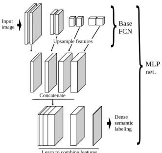
Concatenate

Learn to combine features Upsample features Base FCN MLP net. Dense semantic labeling Input image

Fig. 2: MLP network: intermediate CNN features are con-catenated, to create a pool of features. Another network learns how to combine them to produce the final classification. dilationnetworks [3] uses dilated convolutions (i.e., connect-ing the elements of a convolution kernel to non-contiguous locations of the previous layer) to improve the receptive field size without adding trainable parameters. While this indeed increases the receptive field, it does not provide robustness to spatial variation per se and is computationally demanding.

The category of deconvolution networks [4, 5, 6] adds a series of layers to learn to interpolate and upsample the out-put of an otherwise coarse FCN. This is usually formulated as an encoder/decoder architecture, where a base network is first designed (the encoder) and then a reflected version of itself is attached to it (the decoder, with corresponding “deconvo-lution” and “unpooling” layers). The depth of the network is doubled, making it slower and more difficult to optimize. In addition, it can only recover the lost resolution when the in-dices of the maximal activation of the max-pooling layers are transmitted to the corresponding decoder unpooling layers.

Finally, skip networks [1, 7] create multiple classification maps from different CNN layers (at different resolutions), in-terpolate them to match the highest resolution and add the results to create a final classification map. While the idea of extracting different resolutions is certainly relevant to the principle of Fig. 1, the skip model is arbitrary and insuffi-ciently flexible in how to combine them. We propose next an alternative scheme for high-resolution labeling, leveraging the benefits of the skip network while addressing its potential limitations.

3. LEARNING TO COMBINE RESOLUTIONS Taking multiple intermediate features at different resolu-tions and combining them seems to be a sensible approach to specifically address the localization/recognition trade-off,

as done with skip networks. In such a scheme, the high-resolution features have a small receptive field, while the low-resolution ones have a wider receptive field. Combining them constitutes indeed an efficient use of resources, since we do not actually need the high-resolution filters to have a wide receptive field, following the principle of Fig. 1.

The skip network combines classification maps derived from the different resolutions. We argue though that it is more appropriate to combine features, not classification maps. For example, to refine the boundaries of a coarse building, we may use resolution edge detectors (and not high-resolution building detectors).

Our proposed scheme is depicted in Fig. 2. We depart from a common FCN with convolutional and subsampling layers (the topmost part of Fig. 2). A subset of intermedi-ate features maps is extracted from this network, which are naively upsampled to match the resolution of the higher-resolution features. These maps are concatenated to create a pool of features, emanating from different resolutions, which are treated with equal importance. We must now learn how to combine these features to yield the final classification verdict. For this, a neural network takes as input the pool of features and predicts the final classification map (we could use other classifiers, but this lets us train the system end to end). We assume that all the spatial reasoning has been conveyed in the features computed by the initial CNN, therefore this second network operates on a pixel-by-pixel basis to combine the fea-tures. This way we conceptually and architecturally separate the extraction of spatial features from their combination.

We can think of the multi-layer perceptron (MLP) [8] with one hidden layer and a non-linear activation function as a min-imal system to learn how to combine the pool of features. Such MLPs can learn to approximate any function and, since we do not have any particular constraints, it seems an appro-priate choice. In practice, this is implemented as a sequence of convolutional layers with 1 × 1 kernels, since we want to apply the same MLP at every individual pixel.

The proposed technique, which we refer to as MLP, learns how to combine information at different resolutions. An ex-ample of the type of relation we are able to convey in this scheme is as follows: “label a pixel as building if it is red and belongs to a larger red rectangular structure, which is sur-rounded by areas of green vegetation and near a road”.

4. EXPERIMENTAL RESULTS

We evaluate our architecture on two benchmarks of aerial im-age labeling: Vaihingen and Potsdam, provided by ISPRS1_.

The Vaihingen dataset is composed of 33 image tiles (of av-erage size 2494 × 2064), out of which 16 are fully annotated with class labels. The spatial resolution is 9 cm. The images are split into training and validations sets following [3, 6, 9]. Potsdam dataset consists of 38 tiles of size 6000 × 6000 at

Table 1: Architecture of our base FCN.

Layer Filter size N. of filters Stride Padding

Conv-1 1 5 32 2 2 Conv-1 2 3 32 1 1 Pool-1 2 2 Conv-2 1 3 64 1 1 Conv-2 2 3 64 1 1 Pool-2 2 2 Conv-3 1 3 96 1 1 Conv-3 2 3 96 1 1 Pool-3 2 2 Conv-4 1 3 128 1 1 Conv-4 2 3 128 1 1 Pool 4 2 2 Conv-Score 1 5 1

Table 2: Comparison of our base FCN and derived architectures (Vaihing.)

Imp. surf. Building Low veg. Tree Car Mean F1 Acc. Base FCN 91.46 94.88 79.19 87.89 72.25 85.14 88.61 Unpooling 91.17 95.16 79.06 87.78 69.49 84.54 88.55 Skip 91.66 95.02 79.13 88.11 77.96 86.38 88.80 MLP 91.69 95.24 79.44 88.12 78.42 86.58 88.92

Table 3: Comparison of our base FCN and derived architectures (Potsdam)

Imp. surf. Building Low veg. Tree Car Clutter Mean F1 Acc. Base FCN 88.33 93.97 84.11 80.30 86.13 75.35 84.70 86.20 Unpooling 87.00 92.86 82.93 78.04 84.85 72.47 83.03 84.67 Skip 89.27 94.21 84.73 81.23 93.47 75.18 86.35 86.89 MLP 89.31 94.37 84.83 81.10 93.56 76.54 86.62 87.02

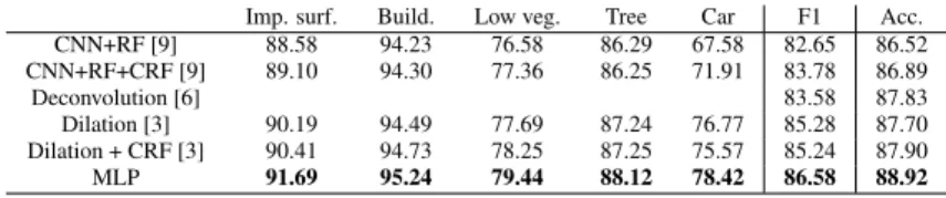
Table 4: Comparison of MLP with other methods on Vaihingen val. set.

Imp. surf. Build. Low veg. Tree Car F1 Acc. CNN+RF [9] 88.58 94.23 76.58 86.29 67.58 82.65 86.52 CNN+RF+CRF [9] 89.10 94.30 77.36 86.25 71.91 83.78 86.89 Deconvolution [6] 83.58 87.83 Dilation [3] 90.19 94.49 77.69 87.24 76.77 85.28 87.70 Dilation + CRF [3] 90.41 94.73 78.25 87.25 75.57 85.24 87.90 MLP 91.69 95.24 79.44 88.12 78.42 86.58 88.92

a spatial resolution of 5 cm, out of which 24 are annotated. Training/validation set is split as in [3]. Both datasets are la-beled into six classes (see Fig. 3). In the case of Vaihingen we predict five classes, ignoring the clutter class, due to the lack of training data for that class. In the case of Potsdam we predict all six classes. In both datasets we use NIR, R, G bands and add the DSM as an extra input channel. In the case of Potsdam we downsample the input and linearly upsample outputs by a factor of 2 (as in [3]), to cover a similar receptive field in terms of meters and not pixels.

To evaluate the overall performance, overall accuracy is used, i.e., the percentage of correctly classified pixels. To evaluate class-specific performance, the F1-score is used, computed as the harmonic mean between precision and re-call [6]. We also include the mean F1 measure among classes. To conduct our experiments, we depart from a base fully convolutional network (FCN) and derive other architectures from it2. Table 1 summarizes our base FCN. Every convolu-tional layer (except the last one) is followed by a batch nor-malization layer [10] and a ReLU activation. To produce a dense pixel labeling we must add a deconvolutional layer to upsample the predictions by a factor of 16, thus bringing them back to the original resolution.

To implement a skip network, we extract the features of layers Conv-* 2, i.e., produced by the last convolution in each resolution and before max pooling. Additional layers are added to produce classification maps from the intermedi-ate features and combined following [1]. Our MLP network was implemented by extracting the same set of features and combining them as explained in Section 3. The added multi-layer perceptron contains one hidden multi-layer with 128 neurons. We also created an encoder/decoder deconvolution network that reflects the base FCN (as in [4]), which we refer to as the unpoolingnetwork.

2_{Code/trained models avail. at github.com/emaggiori/CaffeRemoteSensing}

The networks are trained by stochastic gradient descent. We group five randomly sampled patches (size 256 × 256 for Vaihingen and 512 × 512 for Potsdam), performing random flips and rotations, to compute the gradient in every iteration. We first train the base FCN with a base learning rate of 0.1. We then initialize the weights of the derived unpooling, skip and MLP networks with those of the base FCN, and fine-tune them with a base learning rate of 0.01. Momentum is set to 0.9 and we set the L2 penalty for all parameters to 0.0005.

The classification performances on the validation sets are recorded in Tables 2 and 3. The skip network effectively en-hances the results compared with the base network, while the unpooling strategy does not yield a clear improvement over the base FCN. The MLP network is the most competitive method in almost every case, boosting the performance by learning how to combine features of different resolutions.

As depicted in Table 4, the MLP approach also outper-forms other methods recently presented in the literature, as reported by their authors using the same training/validation sets on Vaihingen.

We submitted the result of executing MLP on the Vaihin-gen test set to the ISPRS server (ID: ‘INR’), which can be accessed online. Our method scored second out of 29 meth-ods, with an overall accuracy of 89.5. Note that the MLP tech-nique described in this paper is very simple compared to other methods in the leaderboard, yet it scored better than them.

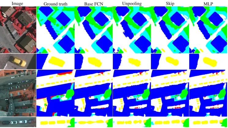
We include visual comparisons on closeups of classified images of both datasets in Fig. 3. As expected, the base FCN tends to output “blobby” objects, while the other methods provide sharper results. The unpooling technique seems to be prone to outputting artifacts. Boundaries tend to be more accurate at a fine level in the case of MLP. For example, the “staircase” shape of one of the buildings in the first row is better outlined by the MLP network.

The inference time is 1.7 s/ha for Vaihingen and 2.0 s/ha for Potsdam. This is, for example, 2.8 and 8.6 times faster

Image Ground truth Base FCN Unpooling Skip MLP

Fig. 3: Classification of closeups of Vahingen (first two rows) and Potsdam (last two rows) validation sets. Classes: Impervious surface (white), Building(blue), Low veget.(cyan), Tree(green), Car(yellow), Clutter(red).

respectively than the dilation network proposed in [3], while providing more accurate results (see Table 4).

5. CONCLUDING REMARKS

With the goal of semantically labeling high-resolution aerial images, we derived a CNN model in which spatial features are learned at multiple resolutions (and thus different levels of detail) and a specific module learns how to combine them. In our experiments, such a model proved to be more effec-tive than other approaches, providing a better accuracy with lower computational requirements. Some of the outperformed methods are in fact significantly more complex than our ap-proach, proving that striving for simplicity is often a relevant approach when using CNN architectures.

6. REFERENCES

[1] Jonathan Long, Evan Shelhamer, and Trevor Darrell, “Fully convolutional networks for semantic segmenta-tion,” in CVPR, 2015.

[2] Emmanuel Maggiori, Yuliya Tarabalka, Guillaume Charpiat, and Pierre Alliez, “Fully convolutional neu-ral networks for remote sensing image classification,” in IEEE IGARSS, 2016, pp. 5071–5074.

[3] Jamie Sherrah, “Fully convolutional networks for dense

semantic labelling of high-resolution aerial imagery,” arXiv preprint arXiv:1606.02585, 2016.

[4] Hyeonwoo Noh, Seunghoon Hong, and Bohyung Han, “Learning deconvolution network for semantic segmen-tation,” in IEEE CVPR, 2015, pp. 1520–1528.

[5] Vijay Badrinarayanan, Ankur Handa, and Roberto Cipolla, “Segnet: A deep convolutional encoder-decoder architecture for robust semantic pixel-wise la-belling,” arXiv preprint arXiv:1505.07293, 2015. [6] Michele Volpi and Devis Tuia, “Dense semantic

label-ing of sub-decimeter resolution images with convolu-tional neural networks,” arXiv prepr.:1608.00775, 2016. [7] Dimitrios Marmanis, Jan D Wegner, Silvano Galliani, Konrad Schindler, Mihai Datcu, and Uwe Stilla, “Se-mantic segmentation of aerial images with an ensemble of CNNs,” ISPRS Annals, pp. 473–480, 2016.

[8] Christopher M Bishop, Neural networks for pattern recognition, Oxford university press, 1995.

[9] Sakrapee Paisitkriangkrai, Jamie Sherrah, Pranam Jan-ney, and Van-Den Hengel, “Effective semantic pixel labelling with convolutional networks and conditional random fields,” in IEEE CVPR Workshops, 2015. [10] Sergey Ioffe and Christian Szegedy, “Batch

normaliza-tion: Accelerating deep network training by reducing in-ternal covariate shift,” arXiv prepr.:1502.03167, 2015.