HAL Id: hal-02895042
https://hal.archives-ouvertes.fr/hal-02895042
Submitted on 9 Jul 2020
HAL is a multi-disciplinary open access
archive for the deposit and dissemination of
sci-entific research documents, whether they are
pub-lished or not. The documents may come from
teaching and research institutions in France or
abroad, or from public or private research centers.
L’archive ouverte pluridisciplinaire HAL, est
destinée au dépôt et à la diffusion de documents
scientifiques de niveau recherche, publiés ou non,
émanant des établissements d’enseignement et de
recherche français ou étrangers, des laboratoires
publics ou privés.
Minimal dynamical systems model of the Northern
Hemisphere jet stream via embedding of climate data
Davide Faranda, Yuzuru Sato, Gabriele Messori, Nicholas Moloney, Pascal
Yiou
To cite this version:
Davide Faranda, Yuzuru Sato, Gabriele Messori, Nicholas Moloney, Pascal Yiou. Minimal dynamical
systems model of the Northern Hemisphere jet stream via embedding of climate data. Earth System
Dynamics, European Geosciences Union, 2019, 10 (3), pp.555-567. �10.5194/esd-10-555-2019�.
�hal-02895042�
0394∆ 8710∆ 0331 014B
Minimal dynamical systems model of the northern hemisphere jet
stream via embedding of climate data
Davide Faranda
1,2, Yuzuru Sato
3,2, Gabriele Messori
4,5, Nicholas R. Moloney
6,2, and Pascal Yiou
1 1Laboratoire des Sciences du Climat et de l’Environnement, UMR 8212 CEA-CNRS-UVSQ, Université Paris-Saclay, IPSL,91191 Gif-sur-Yvette, France
2London Mathematical Laboratory, 8 Margravine Gardens London, W6 8RH, UK
3RIES / Department of Mathematics, Hokkaido University, Kita 20 Nichi 10, Kita-ku, Sapporo 001-0020, Japan 4Department of Earth Sciences, Uppsala University, 752 33, Uppsala, Sweden
5Department of Meteorology and Bolin Centre for Climate Research, Stockholm University, Stockholm, Sweden 6Department of Mathematics and Statistics, University of Reading, Reading RG6 6AX, UK
Correspondence:Davide Faranda (davide.faranda@lsce.ipsl.fr)
Abstract.We derive a minimal dynamical systems model for the northern hemisphere mid-latitude jet dynamics by embedding atmospheric data, and investigate its properties (bifurcation structure, stability, local dimensions) for different atmospheric flow regimes. The derivation is a three-step process: first, we obtain a 1-D description of the mid-latitude jet-stream by computing the position of the jet at each longitude using the ERA-Interim reanalysis. Next, we use the embedding procedure to derive a map of the local jet position dynamics. Finally, we introduce the coupling and stochastic effects deriving from both atmospheric
5
turbulence and topographic disturbances to the jet. We then analyze the dynamical properties of the model in different regimes: one that gives the closest representation of the properties extracted from real data; one featuring a stronger jet (strong coupling); one featuring a weaker jet (weak coupling); and one with modified topography. Our model, notwithstanding its simplicity, provides an instructive description of the dynamical properties of the atmospheric jet.
Copyright statement. TEXT
10
1 Introduction
Jet streams are narrow, fast-flowing westerly air currents near the tropopause. They are a major feature of the large-scale atmospheric circulation and modulate the frequency, severity and persistence of weather events across the extra-tropics (e.g. Röthlisberger et al. (2016)). Their location and intensity also affects commercial aviation and shipping (Reiter and Nania, 1964; Hadlock and Kreitzberg, 1988; Williams and Joshi, 2013). Two types of atmospheric jets can be identified: thermally-driven
15
subtropical jets, and eddy-driven jets associated with baroclinic instability at the polar front. In the Northern Hemisphere (NH), the two are not always clearly separated (Lee and Kim, 2003), and when considering monthly or longer time-averages a single,
spiral-shaped jet structure emerges (e.g. Archer and Caldeira, 2008). In this paper we consider a single NH jet (NHJ), rather than attempting to separate the subtropical and eddy-driven jets (e.g. Belmecheri et al., 2017).
Even though the climatological NHJ is a westerly flow, it can present large meanders on synoptic timescales (e.g. Koch et al., 2006; Röthlisberger et al., 2016). These can cause the local flow to become predominantly meridional, or can even determine a splitting or breaking of the jet (Haines and Malanotte-Rizzoli, 1991). The occurrence of these large meanders in the jet is often
5
associated with events such as temperature and precipitation extremes (e.g. Dole et al., 2011; Screen and Simmonds, 2014). Although jet dynamics are well understood in a climatological sense, our insights into dynamical features such as jet splitting or meandering are still limited.
The dynamics of meanders and split jets has often been framed in terms of transitions between zonal and blocked flows since the seminal work by Charney and DeVore (1979). Legras and Ghil (1985) and Ghil (1987) used an intermediate complexity
10
barotropic model with dissipation forcing and topography, and observed two distinct equilibria associated with the zonal and blocked flows. Similar mechanisms have been proposed by Mo and Ghil (1988) and then performed in experimental facilities (Weeks et al., 2000). However, there is no consensus about the nature of flow multistability, and a wide range of theoretical explanations and models have been proposed (e.g. Tung and Lindzen, 1979; Simmons et al., 1983; Frederiksen, 1982; Faranda et al., 2016b). Moreover, jet dynamics have been described as a manifestation of multiple equilibria in asymmetrically forced
15
flows (Hansen, 1986) or as a result of soliton-modon structures (McWilliams et al., 1981).
In order to advance our understanding of the jet dynamics, we employ a low-dimensional dynamical systems model derived from reanalysis data. The best-known example of a low dimensional model for atmospheric phenomena is Lorenz’ simple three-dimensional system representing some features of Rayleigh-Bénard convection (Lorenz, 1963). Thereafter, simple dynamical systems models have been devised to study El Niño (Penland and Matrosova, 1994), ocean-atmosphere interactions (Dijkstra
20
and Ghil, 2005), climate tipping points (Stommel, 1961; Benzi et al., 1982), large scale atmospheric motions (Lorenz, 1984, 1996) and many other phenomena. The goal of these investigations was not to provide the most realistic representation of the relevant systems, but rather to capture key emerging behaviours (such as chaos, intermittency, multistability). The main drawback of those investigations was the weakness of the connection between models and real data due to the scarcity of observations as well as theoretical limitations. Until very recently, there was a strong case against the use of embedding
25
techniques to derive low dimensional models from experimental data (Letellier et al., 2006). This opposition was motivated by a long sequel of papers that appeared between 1984 and 1991. The initial claim that low dimensional models for complex phenomena could be derived using a very small numbers of variables (see e.g. Nicolis and Nicolis (1984); Fraedrich (1986)) was disproved by rigorous numerical computations by Grassberger (1986) and Lorenz (1991).
Progress in data quality and availability and the advent of stochastic dynamical systems have renewed the attention for
30
data embedding. Recently, Faranda et al. (2017c) have shown that embedding techniques can yield effective low-dimensional dynamics provided that the chosen observables reflect the symmetries of the system and that small-scale (subgrid) dynamics is represented as stochastic perturbations. Here, we use these results to develop a minimal model of the effective dynamics of the mid-latitude jet. This is useful to explore a range of possible behaviors beyond those displayed in the available data, that could have appeared in past climates and could appear again in future climates. In analogy to the model derived by Faranda
et al. (2017c) for the von Karman turbulent flow, the jet model is based on a coupled map lattice (CML, see Appendix A). Each element of the lattice reflects the dynamics of the jet at each longitude. Such a model does not require physical sub-grid terms a priori, but only if they are found to be essential to capture the large-scale phenomenology — which we show is not the case. We then evaluate how this model represents key dynamical features of the jet, namely its stability, the statistics of splitting/breaking and the response to topographical features, and relate the results back to the original ERA-Interim data.
5
First, we provide the details of the ERA-Interim data and of the jet detection algorithm (Section 2). We then present the stochastic coupled lattice map model and compute its bifurcation structure (Section 3). Next, we introduce some instantaneous dynamical indicators (Section 4) and use them to relate the conceptual model to more complex climate models and reanalysis data (Section 5). Finally, we highlight the open questions our results can answer and the new questions they pose (Section 6).
2 Data and Methods
10
2.1 ERA-Interim data and jet position algorithm
The analysis is based on the European Centre for Medium Range Weather Forecasts’ ERA-Interim reanalysis (Dee et al., 2011). We consider daily data with a 1◦horizontal resolution over the period 1979–2016.
The jet position is diagnosed through a modified version of the approach by Woollings et al. (2010). We take daily mean wind-speed averaged over 200–400 hPa and apply a 10-day low-pass Lanczos filter (Duchon, 1979). We then identify the
15
latitudinal position of the jet at every longitude as the location of the strongest wind, over the band 15◦–75◦N. This approach is intended to provide a "raw" measure of the jet variability. We then consider the longitude and time dependence of the latitude of the jet to monitor its waviness.
We define an index of large jet meanders, or breaks (Breaking Index, BRI), as the daily number of meridional variations in jet position of more than 10◦of latitude across adjacent longitude gridpoints, except at longitude 0. The analysis has been
20
repeated for BRI thresholds between 5◦and 15◦, with no significant qualitative differences.
Figure 1 shows a snapshot of the jet position on February 4th 1979, together with the time series of the daily jet position recorded in 1979 at longitude 120◦W. An animation of the jet location for the year 1980 is provided as supplementary video. Both the time series and the snapshot show large jumps in the jet position. A qualitative analysis of the jet position data suggests that the jet fluctuates around a central latitude (Central Jet, CJ) and seldom shifts to more northerly (NJ) or southerly
25
(SJ) latitudes.
In order to embed the data and derive the effective maps of the dynamics, we remove the seasonal cycle from the data by subtracting, longitude by longitude, the average meridional position for each calendar day and dividing by the standard devia-tion. For the deseasonalized data, the dimensionless threshold for the computation of BRI corresponding to about 10◦latitude is|x| > 1.
2.2 Local dynamical systems metrics
Our analysis leverages two recently developed dynamical systems metrics, namely: the local dimension of the attractor d and the stability or persistence of phase-space trajectories θ−1. Instantaneity in time corresponds to locality in phase-space, such that a value of d and θ−1can be computed for a given variable (in our case the jet position data) at every timestep. d is a proxy for the system’s active number of degrees of freedom. It provides information on how the system can reach a given state, and
5
how it can evolve from such state. θ−1describes the persistence of a state in time, thus providing complementary information to d.
2.2.1 Local Dimension
The local dimension is estimated by making use of extreme value statistics applied to Poincaré recurrences. The Freitas et al. (2010) theorem, modified by Lucarini et al. (2012), states that the probability of entering a hyperball with a small radius
10
centred on a state ζ on a chaotic attractor obeys a generalized Pareto distribution (Pickands III, 1975). In order to compute this probability empirically, we first calculate the series of distances dist(x(t), ζ) between the point on the attractor ζ and all other points x(t) on the trajectory. This series is transformed via the distance function:
g(x(t)) =−log(dist(x(t),ζ)), (1)
such that close recurrences of ζ correspond to large values of g(x(t)) (Collet and Eckmann, 2009). Thus, the probability
15
of entering a small hyperball around ζ is transformed into the probability of exceeding a high threshold s(q), where q is a percentile of the series g(x(t)) itself. In the limit of an infinitely long trajectory, it can be shown that the choice g(x(t)) in Eq. (1) locks this probability into the exponential member of the generalized Pareto distribution:
Pr(z > s(q))≃ exp [ −ϑ(ζ) ( z− µ(ζ) β(ζ) )] (2) where where z = g(x(t)), and µ and β (obtained via fitting) depend on the point ζ. These are the location and the scale
20
parameters of the distribution. Remarkably, β(ζ) = 1/d(ζ), where d(ζ) is the local dimension around the point ζ. This result has been recently applied to a range of atmospheric and oceanic fields (e.g. Faranda et al., 2017b, a; Messori et al., 2017; Faranda et al., 2019a, b). In this paper, we use the quantile 0.975 of the series g(x(t)) to determine q. Our results are robust with respect to reasonable changes in this quantile.
2.2.2 Local Persistence
25
Extreme value statistics also allow estimating the persistence of a given state ζ, by inspecting the temporal evolution of the dynamics around it. A measure of persistence around ζ can be obtained from the mean residence time of the trajectory within the neighborhood of ζ. To quantify this, we employ the so-called extremal index ϑ (Freitas et al., 2012; Faranda et al., 2016a):
an adimensional parameter 0 < ϑ(ζ) < 1 which can be interpreted as the inverse of the mean residence time. We can then compute θ−1(ζ) = dt/ϑ(ζ), where dt is the timestep of our data. Heuristically, if the ith visit to the neighbourhood of ζ lasts
τi consecutive time steps, and N such visits are made in total, then θ−1≈ (1/N) ∑
iτi. In practice, instead of this naive estimator, we compute the extremal index using the likelihood estimator of Süveges (2007). θ = 0 corresponds to a stable fixed point of the dynamics, so that the trajectory resides an infinite amount of time in the neighbourhood of ζ. θ = 1 corresponds
5
to a trajectory residing in the neighbourhood of ζ for only one time step per visit. The estimate of θ is thus sensitive to the dt used. If dt is too large, the time dependence structure is unresolved and θ will be close to 1. Conversely, if dt is too small, θ will be close to 0. Faranda et al. (2017b) observed that θ varies between 0.3 and 0.5, when dt = 1 day, for sea-level pressure fields over the North Atlantic. In this work, we use the same dt.
3 Derivation of the lattice jet model
10
3.1 Model Framework
While not directly issued from the Navier-Stokes equations, our framework builds on concrete physical hypotheses, namely that: (i) the physics of the jet is the same at every longitude and it is only slightly modified by the presence of topographical constraints, (ii) the jet can experience sudden breaks and shifts from its central position (CJ) to northern (NJ) or southern lati-tudes (SJ), (iii) the jet must propagate to the west, (iv) smaller scale phenomena, such as turbulence and baroclinic waves, will
15
be introduced in the model only if necessary to reproduce the effective dynamics in the data. This latter point is fundamentally different from the philosophy of direct numerical simulations.
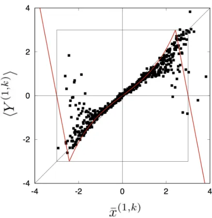
We construct our model starting from the local time series of the non-dimensionalised jet position x measured at each longitude i and time t. We use the simplest possible embedding procedure (see Appendix B), which consists of plotting the return map x(i)t vs. x
(i)
t+1(an example is shown in Figure 2) and searching for a function f
(i)such that x(i)
t+1= f
(i)(x(i)
t ). The
20
first thing to verify is that the same functional form f(i)may be used at all longitudes i. This is equivalent to asking that there is only one dynamics driving the jet independently of the location. With the choice:
f(i)(x) = −A(A+x) A−c + r (i), x <−c, sinh(βx) + r(i), −c ≤ x ≤ c, A(A−x) A−c + r (i), c < x. (3)
where we have dropped the dependecies of x for clarity, the parameters can be fixed at all longitudes as: β = 0.75, A = 3, and
c = sinh−1(A)/β≈ 2.4246. Even though the functional form of f(i)is independent of longitude, a dependence on i remains
25
in the form of the parameter r(i), which represents the effects of topography in terms of spatial inhomogeneities of the local dynamics. As first order approximation, we consider only the difference between land and ocean, and assign one of two discrete values to each r(i). The choice of the function f(i)is not unique; however the one we propose here is a suitable option that
satisfies hypotheses (i) and (ii) above. In order to reproduce the eastward propagation of the jet (hypothesis iii), we introduce the coupled map lattice (CML, see Kaneko (1983) and Appendix A):
x(i)t+1= (1− ϵ)f(i)(x(i)t ) + ϵf(i−1)(x(it−1)), (i = 1, 2, . . . , N ; t = 1, 2, . . .). (4)
With this geometry, the dynamics is divided into N = 360 cells. Periodic boundary conditions are applied at N = 360. The dynamics in each cell i is time-independent, but perturbed by the cell i−1 (i.e. its neighbour to the west) with intensity ϵ, which
5
we estimate and scale based on the observed data. This further implies that our reference length-scale in the model corresponds to that of 1◦longitude in the mid latitudes, namely order 100km.
3.2 Subgrid feedbacks to jet dynamics
If we perform a numerical simulation of Eq. (4), the dynamics is fixed to one of the three states (CJ, SJ, NJ), depending on the
10
value of ϵ. This means that the role of small scales perturbations in triggering the transitions between the states is fundamental. We therefore have to include an additive noise term ξt(i)in Eq. (4):
x(i)t+1= (1− ϵ)f(i)(x(i)t ) + ϵf(i−1)(x(it−1)) + ξt(i), (i = 1, 2, . . . , N ; t = 1, 2, . . .). (5)
The noise is a fundamental ingredient for the breaking of the jet and the transition between zonal and blocked states, as shown in tank experiments and numerical simulations (Jacoby et al., 2011). Physically, noise arises from key sub-grid processes that
15
affect the jet dynamics, such as convection or the interaction between the jet stream and gravity waves (Williams et al., 2003, 2005). Translated to our model with reference spatial scale of order 100km these phenomena, ranging from a few meters to a few kilometers, imply a perturbation in the range 10−4< ν < 10−3. Several subgrid parametrization of turbulence exists: the seminal works of Kraichnan (1961) and Thomson (1987) showed that if large scales are represented by a deterministic term, a single random variable can drive the turbulence term. This means that Langevin model representations are appropriate to
20
describe turbulent eddies (McComb, 1990; Frederiksen and Davies, 1997). Following these ideas, we model νt(i)∈ [−δ,δ] as an uniform random variable.
However, considering small scale turbulent disturbances to the jet dynamics is not sufficient to reproduce the blocking and breaking of the jet. Even if the introduction of ν as a stochastic term can account for the direct Kolmogorov turbulent cascade (Kolmogorov, 1941), the jet dynamics is also driven by the effect of an inverse cascade transferring energy to large scales via
25
baroclinic waves (Held and Larichev, 1996).
Baroclinic activity is associated with extra-tropical cyclones and anticyclones, on scales of order 103km. These can affect
the jet position by several degrees of latitude. Again, there is not a unique way to model baroclinic waves in our framework. We follow the rationale of multiscale parametrizations as they can be theoretically justified (e.g. Wouters and Lucarini (2013); Kitsios and Frederiksen (2019)) and are numerically efficient (Faranda et al., 2014). The simple introduction of another source
of noise η(i), acting at intermidiate scales (i.e. between the scale of the jet and the scale of turbulence), is enough to obtain
a reliable jet breaking dynamics (see Sect. 4.1). The simplest choice for η(i)t ∈ [−µ,µ] is a block noise taking the same value over bl cells (the one-dimensionalized size of cyclones/anticyclones, see Appendix B), and obeying the uniform distribution. Another choice for modelling baroclinic disturbances to the jet could be to introduce a second deterministic equation, weakly coupled with the jet position. However, this choice requires additional hypotheses and parameters and does not emerge naturally
5
from the embedding procedure used to derive the dynamics of x. The minimal sub-grid parametrization can thus be written in the form:
ξt(i)= ν
(i)
t + η
(i)
t , (6)
where ν(i)t and ηt(i)model the effects of small turbulent disturbances and baroclinic eddies, respectively (Figure 3). The noise terms are discussed further in Appendix B.
10
3.3 Local dynamics
Owing to the uni-directional coupling in our model and to the large N , the local dynamics can be approximated by a non-autonomous dynamical system:
x(i)t+1≃ f(i)(x(i)t ) + p(i)t , (7)
where a non-autonomous external force p(i)t is given by:
15 p(i)t = ϵ [ f(i−1)(x(it−1))− f(i)(x(i)t ) ] + νt(i)+ ηt(i). (8)
When|p(i)t | → 0, the local dynamics has a stable fixed point at x ≈ 0, and two unstable chaotic sets near x ≈ ±2. When
p(i)t > 0, the resulting perturbed dynamics may exhibit escape behaviour from the fixed point to the chaotic regions with
pos-itive Lyapunov exponents. Figure 4 shows the bifurcation diagrams as a function of κ over land (r(i)=−0.02), and ocean (r(i)= 0, see Appendix B) obtained by approximating the external perturbation p(i)t as a random variable obeying the uniform
20
distribution in [−κ,κ]. They both indicate a bifurcation to chaotic and partially chaotic behaviour (Sato et al., submitted). The different value of r(i) over land gives rise to an asymmetry in the invariant sets, namely the sets delimiting the accessible region of the dynamics with respect to all possible external perturbations p(i)t . In Figure 4, these dynamically reachable re-gions are depicted in grey, while a realization of the dynamics is depicted by the black dots. With r(i)=−0.02 over land and
0.1574 < κ < 0.1985, there is a small chance to reach SJ positions and no chance to reach NJ positions. This is reflected in
25
the skewed distribution of x(i)t . For the sake of conciseness, we do not report the detailed bifurcation analysis of the local dynamics here. A brief analysis for the global dynamics is presented in Sect. 5.
4 Validation of the model against ERA-Interim data
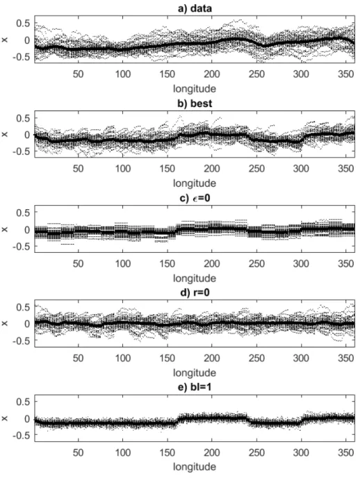
In this section we compare the ERA-Interim deseasonalized jet position data with numerical simulations of our model. In order to have the same statistical sample as as for the reanalysis, we simulate 37 years of daily snapshots of the jet position. The best fit of our model to the data is obtained, by a trial and error procedure, for the parameters: η = 1.2, bl = 15, ϵ = 0.33, δ = 10−4. We further compare the results of model runs containing all noise terms with runs where individual terms are suppressed in
5
turn: the coupling (ϵ = 0), topography (r = 0), and baroclinic waves (bl = 1).
4.1 Spatiotemporal Dynamics
We first consider the latitudinal distribution of the yearly median jet positions at each longitude (dots in Figure 5) and their interannual mean (solid lines in Figure 5). The ERA-Interim dataset (Figure 5-a) presents a negative interannual mean jet position at almost all longitudes, with noticeable zonal asymmetries and a marked interannual variability. The best model run
10
(Figure 5-b) captures both the interannual variability and, thanks to the term r, the longitudinal variations in average location. A run without coupling (ϵ = 0) is shown in Figure 5-c). In this simulation the dynamics is local, except for the presence of block noise, resulting in a discontinuous jet profile. Unlike the ERA-Interim data, the run with no geography (Figure 5-d) has median values which are roughly symmetric around zero. Finally, the run with suppressed baroclinc activity (Figure 5-e) has a smaller interannual variability than the ERA-Interim data and sharp changes in the median values of x following the geographic
15
constraints.
We next consider the NHJ’s shifts from CJ towards NJ or SJ positions. We binarize the dynamics by the detecting all the events such that|x| > 1. Note that this corresponds to breaks in the jet position with the same threshold defined by the breaking index BRI, although there is not exact correspondence. We then assign ’0’ to all the observations with|x| < 1 (CJ) and ’1’ to all the others (NJ or SJ). This procedure, known as coding, is widely used in dynamical systems analysis to identify different
20
dynamical phases in complex systems (Kaneko, 1990). The so-obtained binary spatio-temporal dynamics are shown in Figure 6a-e for all the previously described runs. In the ERA-Interim data (Figure 6a), the switch from CJ to NJ and SJ phases occurs in clusters displaying a characteristic longitudinal extent and temporal persistence. There is also some indication of westerly propagation of the clusters. The best model fit captures the qualitative aspects of this behavior, although the longitudinal coherence is weaker (see section 4.2 below). In the remaining model simulations, the suppression of different noise terms
25
alters either the cluster size or the westerly propagation of the clusters (6c-e). A quantitative analysis of the cluster size spectra is presented in Figure-6f for space clusters and Figure-6g for time clusters. There is a clear power law behavior, reminiscent of a multiscale structure (Schertzer et al., 1997). This is coherent with the claim that the underlying jet dynamics is turbulent, with energy at all scales. Despite its simplicity, our model is reproduces this power law behavior. The theoretical reasons are non-trivial and can be related to the possibility of building turbulent cascades starting from simple Langevin equations (Wouters
30
and Lucarini, 2013; Faranda et al., 2014). We underline here the necessity of adding ϵ and having bl > 1. Indeed when ϵ = 0 the spatial cluster spectrum consist of discrete peaks with the energy concentrated at precises scales. These are a resonance
of the block noise size. When instead we impose bl = 1, we still recover a power-law behavior, but the slope for the temporal clustering strongly deviates from that observed in the ERA-Interim data.
4.2 Dynamical indicators
We further assess our model by means of the d and θ metrics described in Sect. 2.2, computed on both ERA-Interim data and the coupled map lattice. We also compare here the statistics of the spatial breaks of the jet, detected via the indicator BRI.
5
Figure 7 show the box-plots of d (Figure 7-a), and θ (Figure 7-b) for each day in the data set and the breaking index BRI (Figure 7-c). The ranges of values of d and θ for the ERA-Interim data resemble closely those found for sea-level pressure fields over the Northern Hemisphere (Faranda et al., 2017a). This supports the claim that the position of the jet is indicative of large-scale features of the NH atmospheric circulation. Similar claims about the relevance of low dimensional projections in describing the mid-latitude atmospheric circulation are presented by Madonna et al. (2017). The model runs can produce
10
average dimensions comparable to those observed in the ERA-Interim data, except for the bl = 1 case. There, the fragmented dynamics leads to a much higher dimension. This is consistent with the spatio-temporal diagrams shown in Figure 6. The models’ inverse persistence θ are slightly larger than those observed in reanalysis, but still of order 2 days. Here we can clearly see the effect of the noise suppression (ϵ = 0 and bl = 1) in modifying the dynamical properties by leading to lower persistence. Finally, we remark that the number of breaks is correlated to the local dimension. This result is consistent with Faranda et al.
15
(2017b), who found that high d match blocking-like atmospheric configurations in the North Atlantic region. For the limiting
bl = 1 case, BRI is also correlated with θ: the more breaks, the lower the persistence of the flow.
5 Bifurcation diagram and jet regimes
The bifurcation diagram in Figure 8 is constructed by plotting the empirical density ρ(x) of the jet position at all longitudes as a function of ϵ. The vertical gray line corresponds to the value of ϵ that best fits the ERA-Interim data. The diagram would
20
look symmetric with respect to x = 0 if r = 0 everywhere, but the addition of geography via r(i)alters the relative proportions of time spent in SJ versus NJ. Specifically, our asymmetric land/ocean distribution implies a southward shift of the average CJ position with increasing coupling. This is reminiscent of the behaviour in the stochastic bifurcation obtained from the approximated local dynamics (Figure 4). By analysing the bifurcation structure of the conceptual model as a function of the coupling coefficient — which mimics the coherence of the jet — we identify three behaviours: (i) a strong and uniform jet
25
where large meridional excursions in the jet location are relatively rare events (ϵ < 0.35), which is close to the jet dynamics as inferred from the ERA-Interim data; (ii) a state with sharp meridional excursions in which the jet is very unstable and on average shifted far to the South (0.6 < ϵ < 0.9); and (iii) an intermediate state of transition between the two. These jet regimes are broadly consistent with those obtained in idealised atmospheric simulations (Lachmy and Harnik, 2016; Son and Lee, 2005), although here we do not delve into the physical mechanisms underlying the different behaviours. It is also noteworthy
30
that our model qualitatively reproduces a southern jet configuration, even though we provide it with a single NHJ and do not distinguish between eddy-driven and subtropical jets.
6 Conclusions
We have derived a minimal model of the jet stream position dynamics, based on a stochastic coupled map lattice, by embedding data extracted from the ERA-Interim reanalysis. This procedure innovates over earlier studies e.g.(Faranda et al. (2017c)) by making use of a coupled map lattice derived from a local embedding of the data, and could be adapted to systems with several degrees of freedom. Instead of embedding the data of a global observable in a high-dimensional space, we have constructed
5
the return map for the local position of the jet and then added, via coupling and noise, the physical ingredients identified in previous studies as drivers of the jet dynamics. The conceptual model is then validated and tuned using dynamical indicators of the jets dimension and persistence in the reanalysis data.
Future analyses could apply this approach to the southern hemisphere, where the role of topography is less important than in its northern counterpart. This would allow us to better constrain the influence of topography on the dimension-persistence
10
diagrams. Another possibility would be to use the low-dimensional model to build a surrogate data set of the jet positions and then apply this to atmospheric analogues, so as to construct realistic atmospheric dynamics. Finally, it would be interesting to study whether further projections of the atmospheric dynamics to a lower dimensional space are possible, beyond the model developed here, and to test possible relations between different atmospheric blocking indices and the breaking index BRI defined here.
15
The analysis we have conducted can however already answer some of the questions left open in Faranda et al. (2017a) and Madonna et al. (2017) concerning the possibility of reducing the complex mid-latitude circulation dynamics to low-dimensional representations given by blocking indices or conceptual models. The fact that the dimension-persistence diagram of our minimal model qualitatively matches many features obtained for the ERA-Interim jet position and sea-level pressure fields shows that a substantial part of the dynamics projects along a single line (the jet position). This may explain why previous
20
investigations observed relatively low dimensions when considering the full sea-level pressure fields (Faranda et al., 2017b, a). It also suggests that breaks in the jet are responsible for higher dimensions.
Appendix A: Coupled map lattice
A coupled map lattice (CML, Kaneko (1983)) is given by:
x(i)t+1= (1− ϵ)f(x(i)t ) +ϵ 2 [ f (x(it−1)) + f (x(i+1)t ) ] , (i = 1, 2, . . . , N ; t = 1, 2, . . .). (9) 25
where ϵ∈ [0,1], x(i)t ∈ R, and f(x) : R −→ R. For our jet dynamics, we adopt the open flow model, which is class of CML with uni-directional coupling (Kaneko, 1985):
The CML is a phenomenological model to study complex spatio-temporal dynamics in systems with large numbers of degrees of freedom. The idea is to discretize the dynamics in space and time, while capturing the global phenomenology of the system. CMLs have been successfully applied to processes such as turbulence in thermal convection (Yanagita and Kaneko, 1993) and turbulent puff in pipe flow (Avila and Hof, 2013). It is convenient for us to model the jet dynamics leveraging the CML approach because we can extract a local one-dimensional map from the observed time series.
5
Appendix B: Average return map and noise
To extract the local jet dynamics, we construct an average return map. We first coarse-grain the state space into M partitions
L(i)k (k = 1, 2, . . . , M ) and let ¯x(i,k)be the midpoint of L(i)
k . Then, we construct a set Y
(i,k)={x(i) t |x (i) t−1∈ L (i) k } (t = 2,3,...) and a return map f(i)via the return plot of (¯x(i,k),⟨Y(i,k)⟩), where ⟨·⟩ is the average over the elements of Y(i,k) at each longitude i, and at each partition k:
10
⟨Y(i,k)⟩ = f(i)(¯x(i,k)), i = 1, 2, . . . , , N, k = 1, 2, . . . , M, (11)
where|x| ≤ c. In the region |x| > c, we assume linear reflection effects. As a result, we have the return map f(i)in Eq. (3).
Figure 2 illustrates the construction for i = 1 and M = 500.
An important ingredient of the jet dynamics is the presence of topographic obstacles to the mid-latitude zonal flow. Mountain ranges and land-sea boundaries cause meridional deviations in the mean jet location (Tibaldi et al., 1980). This inhomogeneity
15
can be modeled via a parameter r(i)that mimics this “spatial noise”. Since the topography is at most a few kilometers in
height, this translates to a perturbation of the order of 10−3in the model. Reasonable geographical constraints are therefore:
r(i)=−0.02 (i ∈ land) and r(i)= 0.0 (i∈ ocean), where land spans the ranges 0 ≤ i < 161 and 239 ≤ i < 301, and ocean
spans the ranges 161≤ i < 239 and 301 ≤ i < 360. The negative sign for the jet shifts over land is justified by the negative median values of the ERA-Interim jet position anomalies over land (Compare Figure 5-a,b with Figure 5-c where no topography
20
is present).
As discussed in Sect. 3.2, noise is a fundamental ingredient in the jet dynamics. The “turbulent noise” term ν relates to physical phenomena in the range from a few meters to a few kilometers, implying a perturbation in the range 10−4< ν < 10−3, where ν is a random variable obeying the uniform distribution. The second noise term, η, relates to baroclinic activity and we model it as a block noise taking the same value over bl blocks (the one-dimensionalized size of cyclones/anticyclones in our
25
model) with an amplitude of order 1. The latter value is determined empirically as it is an indicative magnitude of the large shifts mid-latitude baroclinic systems can induce in the jet. To determine a realistic length for bl, we reason as follows: given that our model has a reference scale of about 100km, and assuming a typical scale for extra-tropical cyclones of about 3000 km, we then have that bl≈ 30 blocks. However, the perturbations are associated with the cyclone radius rather than diameter: upstream of the cyclone, the jet will mostly be deviated southwards, while downstream of the cyclone, the jet will mostly be
30
Owing to the uni-directional coupling in our lattice jet model and to the large N , the local dynamics can be approximated by a non-autonomous dynamical system x(i)t+1≃ f(i)(x(i)
t )+p
(i)
t , where the external force p
(i) t = ϵ [ f(i−1)(x(i−1) t )− f(i)(x (i) t ) ] +
νt(i)+ ηt(i). Assuming that the time averages⟨f(i−1)(x(it−1))− f(i)(x(i)t )⟩, ⟨νt(i)⟩, and ⟨ηt(i)⟩ are all 0 by symmetry, we have
⟨p(i)
t ⟩ ≈ 0. Thus we recover the average return map given in Eq. (11).
7 Acknowledgments
5
All the authors were supported by the ERC Grant No. 338965-A2C2. DF and YS were supported by the CNRS PICS Grant No. 74774 and by London Mathematical Laboratory External Fellowships. DF and PY were supported by a INSU-CNRS-LEFE-MANU grant (project DINCLIC). YS was supported by the Grant in Aid for Scientific Research (C) No. 18K03441, JSPS, Japan. GM was supported by grant No. 2016-03724 from the Swedish Research Council VetenskapsrÃˇedet, and the Department of Meteorology of Stockholm University. YS, GM and NRM thank the LSCE for the hospitality.
10
Author contributions. DF and YS performed the analysis and derived the conceptual model. GM computed the jet position data. All the
authors participated in the writing and the discussions.
References
Archer, C. L. and Caldeira, K.: Historical trends in the jet streams, Geophysical Research Letters, 35, 2008.
Avila, M. and Hof, B.: Nature of laminar-turbulence intermittency in shear flows, Physical Review E, 87, 063 012, 2013.
Belmecheri, S., Babst, F., Hudson, A. R., Betancourt, J., and Trouet, V.: Northern Hemisphere jet stream position indices as diagnostic tools for climate and ecosystem dynamics, Earth Interactions, 21, 1–23, 2017.
5
Benzi, R., Parisi, G., Sutera, A., and Vulpiani, A.: Stochastic resonance in climatic change, Tellus, 34, 10–16, 1982.
Charney, J. G. and DeVore, J. G.: Multiple flow equilibria in the atmosphere and blocking, Journal of the atmospheric sciences, 36, 1205– 1216, 1979.
Collet, P. and Eckmann, J.-P.: Iterated maps on the interval as dynamical systems, Springer Science & Business Media, 2009.
Dee, D. P., Uppala, S., Simmons, A., Berrisford, P., Poli, P., Kobayashi, S., Andrae, U., Balmaseda, M., Balsamo, G., Bauer, d. P., et al.: The 10
ERA-Interim reanalysis: Configuration and performance of the data assimilation system, Quarterly Journal of the royal meteorological society, 137, 553–597, 2011.
Dijkstra, H. A. and Ghil, M.: Low-frequency variability of the large-scale ocean circulation: A dynamical systems approach, Reviews of Geophysics, 43, 2005.
Dole, R., Hoerling, M., Perlwitz, J., Eischeid, J., Pegion, P., Zhang, T., Quan, X.-W., Xu, T., and Murray, D.: Was there a basis for anticipating 15
the 2010 Russian heat wave?, Mon Weather Rev, 38, 2011.
Duchon, C. E.: Lanczos filtering in one and two dimensions, Journal of applied meteorology, 18, 1016–1022, 1979.
Faranda, D., Pons, F. M. E., Dubrulle, B., Daviaud, F., Saint-Michel, B., Herbert, É., and Cortet, P.-P.: Modelling and analysis of turbulent datasets using Auto Regressive Moving Average processes, Physics of Fluids, 26, 105 101, 2014.
Faranda, D., Alvarez-Castro, M. C., and Yiou, P.: Return times of hot and cold days via recurrences and extreme value theory, Climate 20
Dynamics, 47, 3803–3815, 2016a.
Faranda, D., Masato, G., Moloney, N., Sato, Y., Daviaud, F., Dubrulle, B., and Yiou, P.: The switching between zonal and blocked mid-latitude atmospheric circulation: a dynamical system perspective, Climate Dynamics, 47, 1587–1599, 2016b.
Faranda, D., Messori, G., Alvarez-Castro, M. C., and Yiou, P.: Dynamical properties and extremes of Northern Hemisphere climate fields over the past 60 years, Nonlinear Processes in Geophysics, 24, 713, 2017a.
25
Faranda, D., Messori, G., and Yiou, P.: Dynamical proxies of North Atlantic predictability and extremes, Scientific reports, 7, 41 278, 2017b. Faranda, D., Sato, Y., Saint-Michel, B., Wiertel, C., Padilla, V., Dubrulle, B., and Daviaud, F.: Stochastic chaos in a turbulent swirling flow,
Physical review letters, 119, 014 502, 2017c.
Faranda, D., Alvarez-Castro, M. C., Messori, G., Rodrigues, D., and Yiou, P.: The hammam effect or how a warm ocean enhances large scale atmospheric predictability, Nature communications, 10, 1316, 2019a.
30
Faranda, D., Messori, G., and Vannitsem, S.: Attractor dimension of time-averaged climate observables: insights from a low-order ocean-atmosphere model, Tellus A: Dynamic Meteorology and Oceanography, 71, 1–11, 2019b.
Fraedrich, K.: Estimating the dimensions of weather and climate attractors, Journal of the atmospheric sciences, 43, 419–432, 1986. Frederiksen, J.: A unified three-dimensional instability theory of the onset of blocking and cyclogenesis, J Atmos Sci, 39, 969–982, 1982. Frederiksen, J. S. and Davies, A. G.: Eddy viscosity and stochastic backscatter parameterizations on the sphere for atmospheric circulation 35
models, Journal of the atmospheric sciences, 54, 2475–2492, 1997.
Freitas, A. C. M., Freitas, J. M., and Todd, M.: The extremal index, hitting time statistics and periodicity, Adv Math, 231, 2626–2665, 2012. Ghil, M.: Dynamics, statistics and predictability of planetary flow regimes, in: Irreversible Phenomena and Dynamical Systems Analysis in
Geosciences, pp. 241–283, Springer, 1987.
Grassberger, P.: Do climatic attractors exist?, Nature, 323, 609, 1986.
Hadlock, R. and Kreitzberg, C. W.: The Experiment on Rapidly Intensifying Cyclones over the Atlantic (ERICA) field study: Objectives and 5
plans, Bulletin of the American Meteorological Society, 69, 1309–1320, 1988.
Haines, K. and Malanotte-Rizzoli, P.: Isolated anomalies in westerly jet streams: A unified approach, Journal of the atmospheric sciences, 48, 510–526, 1991.
Hansen, A. R.: Observational characteristics of atmospheric planetary waves with bimodal amplitude distributions, Adv Geophys, 29, 101– 133, 1986.
10
Held, I. M. and Larichev, V. D.: A scaling theory for horizontally homogeneous, baroclinically unstable flow on a beta plane, Journal of the Atmospheric Sciences, 53, 946–952, 1996.
Jacoby, T., Read, P., Williams, P. D., and Young, R.: Generation of inertia–gravity waves in the rotating thermal annulus by a localised boundary layer instability, Geophysical & Astrophysical Fluid Dynamics, 105, 161–181, 2011.
Kaneko, K.: Transition from Torus to Chaos Accompanied by Frequency Lockings with Symmetry Breaking: In Connection with the 15
Coupled-Logistic Map, Progress of Theoretical Physics, 69, 1427–1442, 1983. Kaneko, K.: Spatial period-doubling in open flow, Physics Letters A, 111, 321–325, 1985.
Kaneko, K.: Clustering, coding, switching, hierarchical ordering, and control in a network of chaotic elements, Physica D: Nonlinear Phe-nomena, 41, 137–172, 1990.
Kitsios, V. and Frederiksen, J. S.: Subgrid Parameterizations of the Eddy–Eddy, Eddy–Mean Field, Eddy–Topographic, Mean Field–Mean 20
Field, and Mean Field–Topographic Interactions in Atmospheric Models, Journal of the Atmospheric Sciences, 76, 457–477, 2019. Koch, P., Wernli, H., and Davies, H. C.: An event-based jet-stream climatology and typology, International Journal of Climatology, 26,
283–301, 2006.
Kolmogorov, A.: AN Kolmogorov, Dokl. Akad. Nauk SSSR 30, 301 (1941)., in: Dokl. Akad. Nauk SSSR, vol. 30, p. 301, 1941. Kraichnan, R. H.: Dynamics of nonlinear stochastic systems, Journal of Mathematical Physics, 2, 124–148, 1961.
25
Lachmy, O. and Harnik, N.: Wave and Jet Maintenance in Different Flow Regimes, Journal of the Atmospheric Sciences, 73, 2465–2484, 2016.
Lee, S. and Kim, H.-k.: The dynamical relationship between subtropical and eddy-driven jets, Journal of the Atmospheric Sciences, 60, 1490–1503, 2003.
Legras, B. and Ghil, M.: Persistent anomalies, blocking and variations in atmospheric predictability, J Atmos Sci, 42, 433–471, 1985. 30
Letellier, C., Aguirre, L., and Maquet, J.: How the choice of the observable may influence the analysis of nonlinear dynamical systems, Communications in Nonlinear Science and Numerical Simulation, 11, 555–576, 2006.
Lorenz, E. N.: Deterministic nonperiodic flow, Journal of the atmospheric sciences, 20, 130–141, 1963. Lorenz, E. N.: Irregularity: A fundamental property of the atmosphere, Tellus A, 36, 98–110, 1984. Lorenz, E. N.: Dimension of weather and climate attractors, Nature, 353, 241, 1991.
35
Lorenz, E. N.: Predictability: A problem partly solved, in: Proc. Seminar on predictability, vol. 1, 1996.
Madonna, E., Li, C., Grams, C. M., and Woollings, T.: The link between eddy-driven jet variability and weather regimes in the North Atlantic-European sector, Quarterly Journal of the Royal Meteorological Society, 143, 2960–2972, 2017.
McComb, W. D.: The physics of fluid turbulence, Chemical physics, 1990.
McWilliams, J. C., Flierl, G. R., Larichev, V. D., and Reznik, G. M.: Numerical studies of barotropic modons, Dynam Atmos Oceans, 5, 219–238, 1981.
5
Messori, G., Caballero, R., and Faranda, D.: A dynamical systems approach to studying midlatitude weather extremes, Geophysical Research Letters, 44, 3346–3354, 2017.
Mo, K. and Ghil, M.: Cluster analysis of multiple planetary flow regimes, J Geophys Res-Atmos, 93, 10 927–10 952, 1988. Nicolis, C. and Nicolis, G.: Is there a climatic attractor?, Nature, 311, 529, 1984.
Penland, C. and Matrosova, L.: A balance condition for stochastic numerical models with application to the El Nino-Southern Oscillation, 10
Journal of climate, 7, 1352–1372, 1994.
Pickands III, J.: Statistical inference using extreme order statistics, the Annals of Statistics, pp. 119–131, 1975.
Reiter, E. R. and Nania, A.: Jet-stream structure and clear-air turbulence (CAT), Journal of Applied Meteorology, 3, 247–260, 1964. Röthlisberger, M., Pfahl, S., and Martius, O.: Regional-scale jet waviness modulates the occurrence of midlatitude weather extremes,
Geo-physical Research Letters, 43, 2016. 15
Sato, Y., Doan, T., Rasmussen, M., and Lamb, J. S.: Dynamical characterization of stochastic bifurcations in a random logistic map, arXiv:1811.03994.
Schertzer, D., Lovejoy, S., Schmitt, F., Chigirinskaya, Y., and Marsan, D.: Multifractal cascade dynamics and turbulent intermittency, Fractals, 5, 427–471, 1997.
Screen, J. A. and Simmonds, I.: Amplified mid-latitude planetary waves favour particular regional weather extremes, Nature Climate Change, 20
4, 704, 2014.
Simmons, A., Wallace, J., and Branstator, G.: Barotropic wave propagation and instability, and atmospheric teleconnection patterns, J Atmos Sci, 40, 1363–1392, 1983.
Son, S.-W. and Lee, S.: The response of westerly jets to thermal driving in a primitive equation model, Journal of the atmospheric sciences, 62, 3741–3757, 2005.
25
Stommel, H.: Thermohaline convection with two stable regimes of flow, Tellus, 13, 224–230, 1961. Süveges, M.: Likelihood estimation of the extremal index, Extremes, 10, 41–55, 2007.
Thomson, D.: Criteria for the selection of stochastic models of particle trajectories in turbulent flows, Journal of Fluid Mechanics, 180, 529–556, 1987.
Tibaldi, S., Buzzi, A., and Malguzzi, P.: Orographically induced cyclogenesis: Analysis of numerical experiments, Monthly Weather Review, 30
108, 1302–1314, 1980.
Tung, K. and Lindzen, R.: A theory of stationary long waves. I-A simple theory of blocking. II-Resonant Rossby waves in the presence of realistic vertical shears, 1979.
Weeks, E. R., Crocker, J. C., Levitt, A. C., Schofield, A., and Weitz, D. A.: Three-dimensional direct imaging of structural relaxation near the colloidal glass transition, Science, 287, 627–631, 2000.
35
Williams, P. D. and Joshi, M. M.: Intensification of winter transatlantic aviation turbulence in response to climate change, Nature Climate Change, 3, 644, 2013.
Williams, P. D., Read, P., and Haine, T.: Spontaneous generation and impact of inertia-gravity waves in a stratified, two-layer shear flow, Geophysical research letters, 30, 2003.
Williams, P. D., Haine, T. W., and Read, P. L.: On the generation mechanisms of short-scale unbalanced modes in rotating two-layer flows with vertical shear, Journal of Fluid Mechanics, 528, 1–22, 2005.
Woollings, T., Hannachi, A., and Hoskins, B.: Variability of the North Atlantic eddy-driven jet stream, Quarterly Journal of the Royal 5
Meteorological Society, 136, 856–868, 2010.
Wouters, J. and Lucarini, V.: Multi-level dynamical systems: Connecting the Ruelle response theory and the Mori-Zwanzig approach, Journal of Statistical Physics, 151, 850–860, 2013.
Figure 1.Snapshot of the jet position extracted from the ERA-Interim dataset on February 4th 1979 and time series of the jet position for the year 1979, recorded at longitude 120◦W.
Figure 2. The average return map extracted from the data at longitude i = 1. This is constructed by coarse-graining the state space at
i = 1 into M partitions L(1)k (k = 1, 2, . . . , M ). We then define ¯x(1,k)as the midpoint of the partition L(1)k , and Y(1,k)={x(1)t |x
(1)
t−1∈ L(1)k }
(t = 2, 3, . . .). The black dots represent (¯x(1,k),⟨Y(1,k)⟩) for k = 1,2,...,500, where ⟨·⟩ is the average over the elements of Y(1,k), computed based on the observed data. The red line represents the approximated average return map⟨Y(1,k)⟩ = f(1)(¯x(1,k)), when|x| ≤ c. In the region
|x| > c, we assume linear reflection effects. As a result, we have the return map f(1)
Figure 3.Schematic representation of noise contributions to the CML model (Eq. 3, 6): ν represents local turbulent disturbances, r topo-graphical features, η baroclinic eddies, and i longitudinal positions.
Figure 4. Bifurcation diagrams as a function of κ for (a) land (r(i)=−0.02) and (b) ocean (r(i)= 0.0). The grey regions delimit the accessible region of the dynamics with respect to all possible external forcings. A realization of the dynamics is depicted by the black dots. For r(i)=−0.02 and 0.1574 < κ < 0.1985, there is a small chance to reach SJ positions and no chance to reach NJ positions.
Figure 5.Single-year median location (dotted points) and multi-year average (solid lines) of the meridional jet position for ERA-Interim (a) and model (b-e) data. b) Best-fit model, obtained with η = 1.2, bl = 15, ϵ = 0.33, δ = 10−4, c) as in b) but with ϵ = 0, d) as in b) but with
Figure 6.a-e) Space-time daily representation of the binarized jet dynamics: 1 (black)corresponds to a NJ or SJ shift (|x(t)| > 1) and 0 (white)corresponds to a CJ position. The results are for the ERA-Interim data (a) and model runs (b-e). The latter are the same as in Figure 5. Space (f) and time (g) cluster spectra for the binarized ERA-interim data (black) and the different model runs (colors).
Figure 7.Boxplots of the local dimension d (a), inverse persistence θ (b) and breaking index BRI (c) for the ERA-Interim data and four numerical simulations as in Figure 5. In each box, the central mark is the median, the edges of the box are the 25th and 75th percentiles, the whiskers extend to the most extreme data points not considered outliers, and outliers are plotted individually.
Figure 8.Bifurcation diagram of the global dynamics obtained for η = 1.2, bl = 15, 0 < ϵ < 1, and δ = 10−4. The diagram represents the density of states ρ(x) obtained by varying ϵ. The vertical grey line indicates the value used as best fit to the ERA-Interim data.