HAL Id: hal-01533805
https://hal.inria.fr/hal-01533805
Submitted on 6 Jun 2017
HAL is a multi-disciplinary open access
archive for the deposit and dissemination of
sci-entific research documents, whether they are
pub-lished or not. The documents may come from
teaching and research institutions in France or
abroad, or from public or private research centers.
L’archive ouverte pluridisciplinaire HAL, est
destinée au dépôt et à la diffusion de documents
scientifiques de niveau recherche, publiés ou non,
émanant des établissements d’enseignement et de
recherche français ou étrangers, des laboratoires
publics ou privés.
Avan Suinesiaputra, Pierre Ablin, Xènia Albà, Martino Alessandrini, Jack
Allen, Wenjia Bai, Serkan Çimen, Peter Claes, Brett Cowan, Jan d’Hooge, et
al.
To cite this version:
Avan Suinesiaputra, Pierre Ablin, Xènia Albà, Martino Alessandrini, Jack Allen, et al.. Statistical
shape modeling of the left ventricle: myocardial infarct classification challenge. IEEE Journal of
Biomedical and Health Informatics, Institute of Electrical and Electronics Engineers, 2018, 22 (3),
pp.503-515. �10.1109/JBHI.2017.2652449�. �hal-01533805�
Statistical shape modeling of the left ventricle:
myocardial infarct classification challenge
Avan Suinesiaputra
⇤, Pierre Ablin, X`enia Alb`a, Martino Alessandrini, Jack Allen, Wenjia Bai, Serkan C¸imen,
Peter Claes, Brett R. Cowan, Jan D’hooge, Nicolas Duchateau, Jan Ehrhardt, Alejandro F. Frangi, Ali Gooya,
Vicente Grau, Karim Lekadir, Allen Lu, Anirban Mukhopadhyay, Ilkay Oksuz, Nripesh Parajuli, Xavier Pennec,
Marco Perea˜nez, Catarina Pinto, Paolo Piras, Marc-Michel Roh´e, Daniel Rueckert, Dennis S¨aring, Maxime
Sermesant, Kaleem Siddiqi, Mahdi Tabassian, Luciano Teresi, Sotirios A. Tsaftaris, Matthias Wilms, Alistair A.
Young, Xingyu Zhang and Pau Medrano-Gracia
Abstract—Statistical shape modeling is a powerful tool for visualizing and quantifying geometric and functional patterns of the heart. After myocardial infarction (MI), the left ventricle typically remodels in response to physiological challenges. Se-veral methods have been proposed in the literature to describe statistical shape changes. Which method best characterizes left ventricular remodeling after MI is an open research question. A better descriptor of remodeling is expected to provide a more accurate evaluation of disease status in MI patients. We therefore designed a challenge to test shape characterization in MI given a set of three-dimensional left ventricular surface points. The training set comprised 100 MI patients, and 100 asymptomatic volunteers (AV). The challenge was initiated in 2015 at the Statistical Atlases and Computational Models of the Heart workshop, in conjunction with the MICCAI conference. The training set with labels was provided to participants, who were asked to submit the likelihood of MI from a different (validation) set of 200 cases (100 AV and 100 MI). Sensitivity, specificity, accuracy and area under the receiver operating characteristic curve were used as the outcome measures. The goals of this challenge were to (1) establish a common dataset
Manuscript received June, 2016. This work was supported by award num-bers R01HL087773 and R01HL121754 from the National Heart, Lung, and Blood Institute. AS, BRC and AAY were supported by the Auckland Medical Research Foundation (ref. 1114006). JA was supported by the Medical Research Council (MRC) and Engineering and Physical Sciences Research Council (EPSRC) [grant number EP/L016052/1]. VG was supported by the BBSRC (BB/I012117/1) and a BHF New Horizon Grant (NH/13/30238).
AS, XZ, BRC, AAY and PM-G are with the Department of Anatomy and Medical Imaging, Auckland, New Zealand. WB and DR are with Biomedical Image Analysis Group, Department of Computing, Imperial College London, UK. AM is with Zuse Institute Berlin, Germany. IO and SAT are with IMT Institute for Advanced Studies Lucca, Italy. SAT is also with the University of Edinburgh, UK. JA and VG are with the Institute of Biomedical Engineering, Department of Engineering Science, University of Oxford. PA and KS are with School of Computer Science and Centre for Intelligent Machines, McGill University. KL, MP, and XA are with Department of Information and Communication Technologies, Universitat Pompeu Fabra Barcelona, Spain. SC¸, AG, CP and AFF are with the Center for Computational Imaging and Simulation Technologies in Biomedicine, University of Sheffield, UK. PP is with Department Structural Engineering & Geotechnics, Sapienza, Universit`a di Roma, Italy. LT is with Dept. Mathematics & Physics, Roma Tre University, Italy. MT, MA and JD are with the Department of Cardiovascular Sciences, KU Leuven, Belgium. PC is with the Department of Electrical Engineering-ESAT, KU Leuven, Belgium. MT and MA are also with the Department of Electrical, Electronic and Information Engineering, University of Bologna, Italy. JE and MW are with the Institute of Medical Informatics, University of L¨ubeck, L¨ubeck, Germany. DS is with the University of Applied Sciences Wedel, Wedel, Germany. NP and AL are with the Department of Electrical Engineering and Biomedical Engineering, Yale University, New Haven, CT, USA. M-MR, ND, MS and XP are with the Inria Sophia-Antipolis, Asclepios Research Group, France.
Corresponding author: [email protected]
for evaluating statistical shape modeling algorithms in MI, and (2) test whether statistical shape modeling provides additional information characterizing MI patients over standard clinical measures. Eleven groups with a wide variety of classification and feature extraction approaches participated in this challenge. All methods achieved excellent classification results with accuracy ranges from 0.83 to 0.98. The areas under the receiver operating characteristic curves were all above 0.90. Four methods showed significantly higher performance than standard clinical measures. The dataset and software for evaluation are available from the Cardiac Atlas Project website1.
Index Terms—Cardiac modeling, statistical shape analysis, classification, myocardial infarct.
I. INTRODUCTION
T
HE heart constantly changes its shape and function to maintain normal cardiac output. This process, known as remodeling, can be either adaptive or maladaptive [1]. Adaptive remodeling is a natural process during physiological growth [2] and also commonly seen in athletes [3]. Adverse remodeling, on the other hand, is indicative of the worsen-ing progression of disease. However, the acute response of cardiac remodeling to an insult is usually beneficial, before cardiac function deteriorates into adverse remodeling. Hence, automated characterization and quantification of adverse re-modeling would be a valuable tool for clinicians to quantify the progression of heart disease or to estimate the benefit of a medical treatment.In patients with myocardial infarction (MI), pathophysiolog-ical processes of ventricular remodeling are well studied [4]– [7]. At the early stage of infarction, wall stress increases due to infarct expansion, which forces the left ventricle (LV) to dilate to maintain the supply of blood to the circulatory system. This compensatory LV dilatation is observed by enlargement of cavity volume, both at end-diastole (EDV) and end-systole (ESV). The amount of blood being pumped at each heart beat, which is clinically measured by ejection fraction (EF), is maintained at nearly normal level, irrespective to the infarct size [8]. The amount of LV dilatation, however, depends on the initial infarct size; the greater the infarct size, the greater increase in both EDV and ESV [9].
1http://www.cardiacatlas.org
Prolonged infarction can cause the LV to undergo a more insidious process of dilatation when compensatory remodeling fails to maintain the cardiac output. The loss of myocytes determines further remodeling processes, i.e. a reduction of EF and an increase of ESV [10], [11]. Heart shape also becomes more spherical and less conical [12]. Previous clinical studies have shown that increased ESV and more spherical shapes are predictive of increased mortality after MI [13].
Thus, cardiac remodeling is a continuous process and follow-up monitoring of LV shape and function for MI patients is required to determine the efficacy of treatment or time interventions [14]. Standard measurements commonly used to assess cardiac shape and function (termed baseline in this paper) are LV cavity volumes, particularly EDV and ESV, LV mass and EF [15]. MRI is the gold standard method for quantification of these measures [16]. However, these simple shape features ignore much of the shape information available in modern MRI examinations. We hypothesized that statistical shape modeling methods, using supervised or unsupervised dimension reduction methods, could provide additional infor-mation for the evaluation of MI patients over the baseline measures. We initiated an open challenge to automatically estimate shape features, and compare their performance in a blinded test to distinguish MI patients from asymptomatic volunteers. Eleven research groups participated in the chal-lenge, as part of the 6th Annual Workshop of Statistical Atlases and Computational Models of the Heart (STACOM) held in conjunction with MICCAI 2015 conference [17]. This paper collates the challenge results together with the baseline prediction model, and discusses the main advantages and disadvantages of the different approaches.
A. Motivation of the challenge
Although there has been a lot of work on statistical shape analysis over the last 10-20 years in our community, clinical applications are only now being explored [18], as clinical indices are still mostly measured in 0D, 1D or 2D. There is therefore a growing interest in the medical imaging community to apply machine learning algorithms to assist clinical evalu-ation of real patient data. Open challenges using substantial clinical data, comparing many different methods, are crucial to convince clinicians of the benefit of using the full shape information with statistical shape features [19].
In this challenge, we focused on the statistical analysis of LV shape and function after MI. Previous studies have demonstrated the efficacy of statistical shape analysis to automatically predict, locate and quantify abnormal cardiac shapes and function in different pathological groups. Zhang et al. [20] classified patients with myocardial infarction by using information maximization component analysis applied to the LV surface points. Ardekani et al. [21] analysed statistical variations of LV surface deformations in hypertensive and hypertrophic heart disease. Zhang et al. [22] used surface point distributions from active shape and appearance models, while Ye et al. [20] applied regional manifold learning, to quantify congenital heart disease remodeling relative to normal volunteers. Manifold learning was also used by Duchateau et
al. [21] to identify patients that responded to resynchronization therapy and by Piras et al. [23] to extract features of normal LV motion. Other statistical cardiac shape methods have also been proposed [24]–[28].
Apart from statistical shape features, there has been con-siderable work in modeling cardiac shape and motion, which can be used to extract shape descriptors. A deformable su-perquadric model fit by a free-form deformation can reveal differences in LV shape deformation [29]. A spherical har-monic model was applied to extract shape descriptors for 3D heart surface [30]. A general deformable model can be used to characterize different motion of the heart [31]. A review of shape models can be found in [32]. With a growing number of algorithms for the analysis of pathological heart shapes, therefore it is an urgent need to create a benchmarking platform to compare the relative efficacy of different methods. B. The challenge objectives
We hypothesized that automated shape characterization methods perform better than the baseline measures, since multidimensional information about the LV shapes and their variations within a pathological group can be incorporated into the shape model. We aimed to discover what shape features best describe the adverse remodeling of the LV after MI in comparison with the baseline measures.
The challenge data consisted of 200 cases from a cohort study that studied MI patients [33] and another 200 cases from a different cohort that studied asymptomatic volunteers (AV) [34]. In total, there were 400 LV shapes made available for this challenge. Participants were asked to provide the degree of disease from these cases in terms of the likelihood that the LV shape describes an MI patient. The dataset was randomly divided into training and validation sets; each par-ticipant was able to use the training set with open labels for learning. No other information was provided.
Although the primary challenge objective was to examine methods for quantifying degree of pathology, classification of MI is not typically performed solely from shape and motion in clinical practice. Common methods include tro-ponin levels, late gadolinium enhancement, stress perfusion or motion abnormalities, and angiography. However, this chal-lenge represents an extremely valuable opportunity to build a reduced space in which more complex phenomena like longitudinal evolution can be studied. Therefore, the main clinical application of these statistical shape analysis methods will be in quantifying the progress of remodeling, for example as a z-score showing how the patient ranks against progressing severity of disease. Participants were therefore asked to pro-vide a likelihood for the presence of MI, which could be used to evaluate the severity of disease against population norms, or in longitudinal studies to evaluate the progression of disease. The remainder of this paper is organized as follows. Section II describes the data and evaluation design of this challenge. In Section III, we briefly describe each participa-ting method. Full details of their methodology are explained in [17]. Section IV compares the classification results. Finally, Section V discusses several aspects of this challenge, including
TABLE I
DEMOGRAPHICS OF THE CHALLENGE DATASET. CONTINUOUS VARIABLES ARE EXPRESSED AS MEAN(STANDARD DEVIATION). STATISTICAL TESTS
WERE PERFORMED WITHWILCOXON SIGNED-RANK TEST FOR CONTINUOUS VARIABLES AND 2 TEST FOR CATEGORICAL VARIABLES. A
SYMBOL FOR † DENOTESp < 0.05FOR TESTS BETWEEN TRAINING AND VALIDATION SETS. SBP =SYSTOLIC BLOOD PRESSURE, DBP =
DIASTOLIC BLOOD PRESSURE, HR =HEART RATE, HYP=HYPERTENSION, DBT=DIABETES, SMK=SMOKING.
AV (n=200) MI (n=200)
Training Validation Training Validation
n=100 n=100 n=100 n=100 Sex 41M/59F 49M/51F 81M/19F 81M/18F Age 62.5 (9.4) 59.3 (9.4) 63.3 (10.8) 62.8 (12.3) Height 167.5 (9.6) 164.5 (9.4) 173.6 (10.1) 174.1 (9.9) Weight 80.8 (16.0) 76.6 (15.1) 88.2 (18.3) 90.3 (19.2) SBP 129.9 (24.7)† 120.0 (22.1) 122.2 (19.7)† 130.1 (19.7) DBP 72.3 (10.8) 69.7 (9.9) 72.4 (11.7) 73.4 (11.9) HR 62.1 (12.2) 60.4 (10.7) 66.0 (11.6) 65.9 (10.9) EDV 114.2 (22.8) 117.4 (23.6) 188.3 (45.2) 202.2 (55.2) ESV 45.5 (14.3) 45.9 (13.4) 109.3 (41.5) 125.6 (54.5) LVM 137.1 (38.6) 136.8 (31.4) 161.8 (37.5) 174.2 (44.4) EF 60.6 (5.8) 61.3 (5.5) 43.4 (10.4) 39.9 (11.9) Hyp 48% 39% 71% 70% Dbt 18% 24% 37% 38% Smk 45% 51% 73% 70%
the most misclassified cases, useful features, and some limita-tions of this challenge. Conclusions and future direclimita-tions are given in Section VI. Data and evaluation software will remain open to researchers at the Cardiac Atlas Project website [35].
II. DATA ANDEVALUATION
A. Patient Data
We randomly selected 400 cases from two main cohorts: MESA (Multi-Ethnic Study of Atherosclerosis) and DETER-MINE (Defibrillators to Reduce Risk by Magnetic Resonance Imaging Evaluation). Data were retrieved from the Cardiac Atlas Project database [35]. The MESA cohort [34] consisted of asymptomatic volunteers (n=200), since they did not present any clinical symptoms of cardiovascular disease at recruitment. The DETERMINE cohort [33] consisted of patients with clinical evidence of myocardial infarction (n=200). The dataset was randomly split into 200 cases for training and 200 cases for validation (Table I).
We provided classification labels only for the training set (0 = AV, 1 = MI). Therefore, for training purposes, participants could only estimate their cut-off threshold value for binary classification from the training dataset. However, there was no requirement to use the training dataset in their algorithm. Participants were asked to provide either classification labels or probability values that a case is an MI from the validation set.
ED ES
Fig. 1. Example of the supplied data points in patient coordinate system. Finite-element models were subdivided using a high-resolution lattice result-ing in 1,089 points per surface. The epicardial surface is shown in red, the endocardium in black/green. The contractile motion can be observed from the difference between end-diastole (ED) and end-systole (ES).
B. Shape Data
In this challenge, we aimed for participants to only focus on shape features and classification. Therefore, we provided a set of 3D points in Cartesian coordinates from the surface of LV shapes, which has point-to-point correspondences between shapes. First, we used custom-made software package (CIM version 6.0, University of Auckland, New Zealand) to fit a finite element LV model [47] onto cine MR images. The fitting was performed interactively by two expert analysts using guide-point modeling technique with inline feature track-ing [48]. Since the models were registered to the anatomical landmarks of each heart, the finite element model coordinates were treated as homologous points in the LV.
Evenly spaced homologous points were generated covering ventricular surfaces, resulting in 2,178 Cartesian points in pa-tient coordinates. Only surface points from end-diastole (ED) and end-systole (ES) frames were given to the participants. Figure 1 shows an example of mesh triangulation visualization for the endocardial and epicardial surfaces from the supplied data points. Since images for the AV group were acquired using a different imaging protocol (Gradient Recalled Echo or GRE) than the MI group (Steady-State Free Precession or SSFP), the AV shape models were corrected for protocol bias using the method described in [49]. This method corrected for acquisition bias on a regional point-by-point basis, and has been shown to not only correct for regional shape bias but also global bias in mass and volume. The sensitivity analysis performed in [49] confirmed that enough training cases were included to robustly identify the mapping parameters, since the correction only pertains to the asymptomatic group. After the correction, the transformed AV shape models were then directly comparable to the MI shape models.
C. Baseline
A baseline prediction model was introduced to provide a benchmark to assess the clinical benefit of the participating algorithms. We selected EDV, ESV, LVM and EF from Table I because these are widely-used clinical indicators and are known to be markedly changed due to MI. We applied a binary
TABLE II
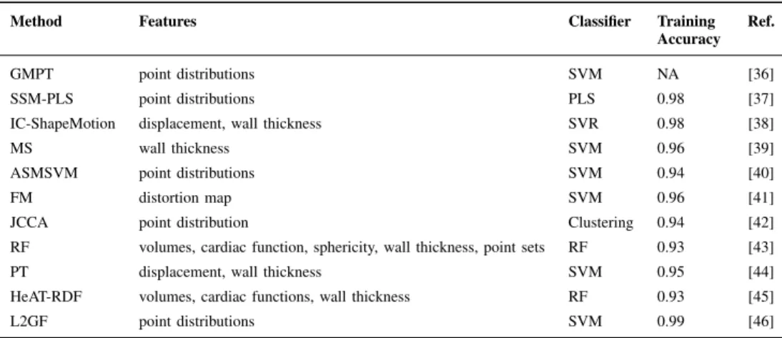
SUMMARY OF EACH PARTICIPATING METHOD. SVM = SUPPORTVECTORMACHINES, PLS = PARTIALLEASTSQUARES, RF = RANDOMFOREST, SVR = SUPPORTVECTORREGRESSORS.
Method Features Classifier Training
Accuracy Ref.
GMPT point distributions SVM NA [36]
SSM-PLS point distributions PLS 0.98 [37]
IC-ShapeMotion displacement, wall thickness SVR 0.98 [38]
MS wall thickness SVM 0.96 [39]
ASMSVM point distributions SVM 0.94 [40]
FM distortion map SVM 0.96 [41]
JCCA point distribution Clustering 0.94 [42]
RF volumes, cardiac function, sphericity, wall thickness, point sets RF 0.93 [43]
PT displacement, wall thickness SVM 0.95 [44]
HeAT-RDF volumes, cardiac functions, wall thickness RF 0.93 [45]
L2GF point distributions SVM 0.99 [46]
multiple logistic regression [50] to model the effects of these clinical parameters on the probability that a case belongs to the MI group.
By using the 200 cases from the training set, the baseline model was given by
ln ✓ p(X) 1 p(X) ◆ = 0+ 1XEDV+ 2XESV+ 3XLVM+ 4XEF (1) where the intercept 0 = 12.35 and the contributions of
each variable were 1 = 0.11, 2 = 0.09, 3 = 0.03
and 4 = 0.31. The largest effect was given by LVM
(P < 0.001), followed by EDV (P < 0.05). The prediction model (1) was estimated by using the glm (generalized linear model) function from the standard R package. To perform the logistic regression with glm, a binomial distribution was set as the distribution family parameter.
D. Evaluation
Method performance was meassured by means of specificity (spec), sensitivity (sens), and accuracy (acc) [51]. Let TP, TN, FP and FN be the number of true positives, true negatives, false positives and false negatives, respectively. These performance measurements are then defined as
sens = TP TP + FN (2) spec = TN TN + FP (3) acc = TN + TP TN + TP + FN + FP (4) In this study, a positive denotes an MI shape, while a negative is an AV shape. Hence, the sensitivity measures how good a classifier correctly identifies MI shapes from the MI group, while specificity eliminates AV shapes from being identified as MI. The combination of sensitivity and specificity determines the accuracy of a classifier.
Receiver Operating Characteristic (ROC) curves were gen-erated by the ROCR package [52]. The area under the ROC
curve (AUC) is a useful measure of the overall method performance. To calculate individual performance, the optimal cut-off value for classification was estimated by using the Youden index J [53], [54], which is defined as
J = max
c {sens(c) + spec(c) 1} (5)
where c is the cut-off value ranging from 0 to 1. The Youden index basically maximises both sensitivity and specificity values, resulting in a point on an ROC curve, which gives the maximum distance to the diagonal line. This method was performed to provide an objective measure of the ROC curve, which was calculated from the likelihoods provided by the participants. Since the objective was to provide an objective measure of remodelling, rather than identify MI, we did not impose a priori thresholds in the test dataset. Statistical tests between methods were performed by using one-sided paired non-parametric test for AUC values [55], implemented in the pROCpackage [56]. A p < 0.05 defines a statistically higher AUC value than the baseline model.
III. PARTICIPATINGMETHODS
There were a total of 11 participant groups [17]. Table II summarizes and compares attributes of the different algo-rithms. Some methods used similar feature sets and classi-fiers, but there were differences in how they pre-processed, trained and extracted features from the datasets. The following subsections briefly describe each algorithm. In each case we have a provided a reference for readers to find a more detailed explanation of the methodology and parameters used. A. GMPT: Systo-diastolic LV shape analysis by Geometric Morphometrics and Parallel Transport
Description: This method combined geometric morphomet-rics approach with parallel transport to extract features from ED and ES shapes. Geometric morphometrics is a common framework in statistical shape analysis, which exploited sta-tistical variations of homologous points on 2D/3D shapes
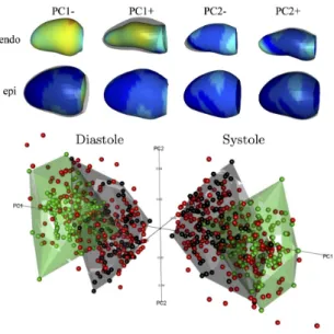
Fig. 2. PCA results from theGMPT method. Top: 3D shapes corresponding to PC1 and PC2 modes, coloured according to the distance with respect to the average mean shape (blue: minimum; red: maximum). Bottom: Shapes in the PC1-PC3 space in ED (left) and ES (right); green=AV from training, black=MI from training, red=validation set.
after the removal of shape preserving transformations by using Generalized Procrustes Alignment (GPA) [57]. Principal component analysis (PCA) was applied to the aligned shapes to extract the shape features.
Features: Surface point sets in the form of a shape vector [x1, y1, z1, . . . , xN, yN, zN]T. ED and ES shapes were treated
as different shapes, resulting in total of 800 shapes. Different combinations of GPA, PCA, parallel transport, scale removal, shape centering, endocardium, epicardium, and the full shape (endocardium + epicardium) were explored during training.
Classifiers: Five classifiers were explored: linear discrimi-nant analysis, logistic regression, quadratic discrimidiscrimi-nant ana-lysis, random forests and support vector machines. With the combination of features, 30 different types of analysis were reported in [36]. No information was given about parameters used in these classifiers.
Submission: The best combination of feature extraction and classifier method was given by support vector machines using a sequence of GPA + parallel transport + PCA on the full LV surfaces (both endocardium and epicardium) centered at the average shape in the shape space (see Fig. 2). This method was contributed by PP and LT [36].
B. SSM-PLS: Statistical Shape Modeling using Partial Least Squares
Description: This method applied partial least squares (PLS) regression approach for statistical shape models (SSM) to extract axes of shape variation that correlated most with the MI classification. This SSM-PLS method was able to decompose clinically meaningful axes, which were statistically optimal for prediction purposes. Furthermore, to increase the accuracy of the MI classification, several PLS classifiers were
Fig. 3. First mode of PLS variation obtained for the endocardium at ED from
theSSM-PLS method.
fused together by varying the number of new axes of variation during the PLS decomposition.
Features: PLS regression coefficients of the surface point sets with a binary label. During regression, the LV surface points were set as the predictor matrix X, which were then regressed into a single binary variable Y as the response matrix. This variable is the labelling values of either AV or MI shape.
Classifiers: PLS regression with varying numbers of latent variables. The final classifier was determined by calculating the median value from a set of PLS classifiers.
Submission: The training achieved accuracy of 0.98, speci-ficity of 0.99 and sensitivity of 0.97. Fig. 3 shows the first mode of PLS variation for the endocardium at ES. The figure describes variation from significant cardiac motion ( 2 ), typical in healthy subjects to less pronounced cardiac motion due to infarcted muscle (+2 ), where is standard deviation. This method was contributed by KL, MP, XA, and AFF [37]. C. IC-ShapeMotion: Classification of myocardial infarction by combining shape and motion features
Description: This method combined shape and motion as a feature set for a support vector regressor (SVR) classifier. Instead of raw surface point set, the shape features were extracted from 3D surface mesh. The motion feature was defined in terms of wall thickness, wall thickening and vertex displacement.
Features: 1) Shape: ED surface mesh models were aligned using a rigid registration method, and then this transformation was applied for the ES mesh model. PCA was performed on the aligned ED and ES meshes separately to extract the principal coefficients PED and PES. The concatenated
P = [PED, PES] was also introduced. 2) Wall thickening:
absolute Ta = (wES wED) and relative Tr = Ta/wED.
3) Wall displacement, defined as vertex displacement from ED to ES meshes. The displacement was measured in radial (Dendo,r, Depi,r), longitudinal (Dendo,l, Depi,l) and
circumfer-ential (Dendo,c, Depi,c) directions.
Classifiers: Support vector machines with radial basis function kernel. Training was performed on 10-fold cross validation scheme.
Submission: The best feature set was given by {P, Ta, Dendo,c, Depi,r}, which resulted in 0.98 accuracy,
0.98 sensitivity and 0.97 specificity. This algorithm was contributed by WB and DR [38].
D. MS: Detecting MI using Medial Surfaces
Description: A medial surface is a skeleton representation of a 3D object defined by a set of maximal inscribed disks within the object. The medial representation of an LV shape is therefore a mid surface between endocardium and epicardium, which was modeled as a fixed single sheet topology [58]. This was calculated by using a voxelization technique. The resulted medial surface contained radius values at each voxel. Medial surfaces at ED and ES were subsequently aligned using the coherent point drift algorithm, and then each registered pair was further aligned to a reference heart.
Features: Radial values (wall thickness). ED and ES radial values were concatenated for each shape. PCA was used to reduce the number of features from 10000 to 100.
Classifiers: 1) Support vector machines with radial basis function kernel. Training was performed on 40-fold cross validation scheme. 2) Random forest.
Submission: The support vector machines classifier achieved the best result with 0.96 accuracy, which was then selected for submission. The random forest classifier only achieved 0.88 accuracy. This method was contributed by KS and PA [39].
E. ASMSVM: Active shape model and support vector ma-chine
Fig. 4. TheASMSVM method: (a) Alignment of an LV shape (right) to the
reference LV shape (left) (b) PCA decomposition (c) SVM classification into AV ans MI.
Description: This method applied the active shape model [59] approach combined with support vector ma-chines for classification. First, ED LV shapes were aligned to a common reference LV. Since points were already reg-istered anatomically, point-to-point correspondence step was not needed. The same transformation that aligned ED LV was applied to the corresponding ES LV shape to maintain relative differences.
Features: PCA coefficients from the aligned surface point sets.
Classifiers: 1) Support vector machines with radial basis function kernel and 2) linear support vector machines. The kernel weight was modified to be inversely proportional to the distance of a shape from the mean shape. Training was performed on 10-fold cross validation scheme.
Submission: The radial basis function kernel was chosen for submission as it achieved a slightly better sensitivity than the linear kernel. The overall training performance was 0.94 accuracy, 0.94 sensitivity and 0.93 specificity. Figure 4
Fig. 5. Distortion maps from theFM method over the whole population of
AV and MI groups from the training dataset at various scales k.
summarizes the overall method. This method was contributed by NP and AL [40].
F. FM: Supervised learning of functional maps
Description: This method was based on the observation that changes in the LV shape resulted in a distortion of the 2D surface area embedded in 3D space. Features were then deter-mined from the LV surface parameterized by a functional map, which represents a mapping between two bijective shapes. By using harmonic analysis, a set of Fourier coefficients can be used to represent the correspondence between two shapes. This correspondence representation can further be approximated using k basis functions, encoded in k ⇥ k functional matrix. Figure 5 shows the distortion maps at ED and ES from both groups at different k scales. The goal was to isolate the regions where the map has induced significant distortion at various scales by performing spectral analysis of this representation.
Features: Surface areas from the functional maps that produced significant distortions between ED and ES. This was computed by subtraction of the total areas of ED from ES. Each endocardium and epicardium surface was treated separately.
Classifiers: Support vector machines. No information about the kernels and parameters were provided. Training was per-formed on 10-fold cross validation scheme.
Submission: The training achieved accuracy of 0.96±1.26. This method was contributed by AM, IO and SAT [41]. G. JCCA: Joint Clustering and Component Analysis of spatio-temporal shape patterns
Description: This method used a hierarchical generative model [60] with two layers to extract features for classification. At the lower level, a Gaussian Mixture Model was used to estimate the probability density functions of the surface point sets. The mean values of each model were then concatenated to create a vector. A probabilistic principal component analyzer method [61] was applied to create two clusters (AV and MI clusters) from these vectors at the higher level.
Features: Resampled point sets from the estimated clusters at the higher level. The LV shapes were first aligned by using the coherent point drift algorithm. ED and ES shapes were concatenated.
Classifiers: Both unsupervised and supervised learning were explored. Variational Bayesian was used for the unsuper-vised clustering to estimate mean and variance of the clusters. Submission: The performance between unsupervised and supervised clustering were 0.90 vs 0.94 for accuracy, 0.97 vs 0.97 for sensitivity and 0.83 vs 0.91 for specificity. The supervised clustering was therefore chosen for submission. This method was contributed by AP, SC¸, AG and AFF [60]. H. RF: MI detection from LV shapes using Random Forest
Feature Index
0 5 10 15 20 25 30 35 40 45 50 55 60 65 70
'Out-of-Bag' Feature Importance
0 0.5 1 1.5
Ejection Fraction
Dia. Sys. Shape Mode 13
Thickness Change Variance Sys. Endo. Volume Log Sys. Endo. Volume
Dia. Sys. Thickness Mode 7
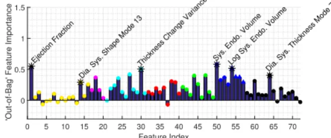
Fig. 6. Important feature selection by theRF method.
Description: This method combined standard clinical func-tion (volumes, ejecfunc-tion fracfunc-tion, sphericity) and novel atlas-based metrics (shape, myocardial thickness) as features for a Random Forest (RF) classifier. Figure 6 shows the importance values of each feature, showing a clear predominance of ejec-tion fracejec-tion but also the presence of important classificaejec-tion information in certain shape and thickness modes.
Features: A total of 72 features were included: ejection fraction, the first 15 PCA shape modes, sphericity, mean thickness, mode thickness, mean thickness, wall thickness variance and its differences, mean and variance of thickness values based on segments (apex, middle and base), epicardial and endocardial volumes, the log volumes and the first 15 PCA modes of thickness.
Classifiers: Random forest with 5-fold and 20-fold cross validation schemes.
Submission: The 15 features with the largest importance were chosen as features to build the final random forest. The training accuracy was 0.93. This method was contributed by JA and VG [43].
I. PT: Combination of polyaffine transformations and super-vised learning
Description: This method relies on a parametric model of diffeomorphic deformations of the heart based on polyaffine transformations. Polyaffine transformations represent the heart motion by the combination of a limited number of affine transformations defined locally on a regional division of the space (in the case of the heart the American Heart Association (AHA) myocardial segmentation definition [62] was chosen).
These transformations not only serve as a first (non-learnt) dimension reduction, but can also be linked to known clinical parameters (strain and displacement along the 3 dimensions). Features: Polyaffine parameters (strain and displacement, each in radial, circumferential and longitudinal directions) and regional thickness at both ED and ES.
Classifiers: Decision trees, random forest, logistic regres-sion, nearest neighbours, linear and radial basis function kernel support vector machines. For each classifier, two different reduction algorithms were used: PCA and PLS regression. The training used 10-fold cross validation scheme.
Submission: The best classifier was given by support vector machines with radial basis kernel functions on PLS regression that achieved 0.95 accuracy. This method was contributed by M-MR, ND, MS and XP [44].
J. HeAT-RDF: Automatic detection of cardiac remodeling using global and local clinical measures and random forest classification
Description: This method explored different shape and clinical parameters for cardiac shape classification in the Heart Analysis Tool (HeAT) framework, combined with random forest classifier (HeAT-RDF). A large range of global and local clinical parameters were extracted based on endocardial and epicardial contours using custom-made software tool. The software has been primarily developed for analysis of contours extracted from image data. The triangulated shapes from this challenge data were first converted to contours by placing 10 short-axis planes between the most basal and the most apical points on the ED shapes. The resulting contour points were interpolated to generate smooth continuous contours per slice. A 97 segment model with higher resolution was used for local analysis. Corresponding points in the middle of the septum were utilized to define corresponding segments across all patients.
Features: Five global and 388 local LV functions were extracted as features during training. The 10 most important features selected for the challenge validation set were ESV, myocardial thickness (segment 95), EDV, EF, motion ampli-tude endocardium (segment 94 and 85), contraction of the endocardium (segment 85), change in wall thickness (segment 85, 80 and 50).
Classifiers: Random forest with parameters of 400 decision trees and a maximum of 50 depth.
Submission: The training achieved 0.93 accuracy, 0.93 specificity and 0.92 sensitivity. This method was contributed by JE, MW, and DE [45].
K. L2GF: Automatic detection of MI through a global shape feature based on local statistical modeling
Description: This method combined global and local shape decomposition with PCA to extract features for the LV shape classification. The rationale for local shape analysis was: 1) to better identify abnormalities that lead to local shape remodeling and, 2) to decrease the number of shape variables by using a limited set of points. The LV was first divided into regions of interest (ROI) to learn local shape components
Feature Concatenation Classification
Segment n Segment 1
Local PCA 1 Feature
Selection
Local PCA n Feature
Selection
Fig. 7. L2GF method. Independent PCA models were built with the local
shape components and a subset of the trained parameters with significant discriminatory information was taken from each local model in a feature selection stage. The selected parameters were then concatenated to train a support vector machine classifier.
where each ROI was composed of endocardial and epicardial shapes at ED and ES. PCA was subsequently used to reduce the dimension. A subset of the PCA-derived parameters that provided significant discriminatory information was selected from each local model using the P -metric feature selection method [63]. The selected parameters were then concatenated to form a global representation of the LV. In this way, global shape parameters were encoded and the spatial relation between the local zones was also taken into consideration. This approach is shown in Fig. 7.
Features: Global and local PCA coefficients. Local PCA decompositions were calculated from three different sizes of region of interest: 4, 8 and 16 surface faces.
Classifiers: Support vector machines with linear kernels. Training was performed on 10-fold cross validation scheme.
Submission: The training achieved 0.99 accuracy. This method was contributed by MT, MA, PC, and JD [46].
IV. RESULTS
Table I shows the demographics, traditional risk factors (hypertension, history of smoking and diabetes) and cardiac functional parameters including end-diastolic volume (EDV), end-systolic volume (ESV), LV mass (LVM) and ejection fraction (EF) of both datasets for both groups. We tried to match the distribution of training and validation sets for both asymptomatic volunteers (AV) and myocardial infarction (MI) groups as close as possible. No significant differences were found between training and validation dataset, except for systolic blood pressure (Bonferroni corrections applied). Significant differences were present in many risk factors, male/female distribution, and age between AV and MI, since these were two different population groups and we were not able to control for these factors. While these factors are known to have effects on LV mass and volume, these are expected to be outweighed by disease processes [20], [28]. Also, controlling for risk factors may not be desirable since these could be linked to clinically important manifestations of disease.
All methods, with the exception of one (L2GF), provided MI shape probability values for the validation dataset. Table III compares classification performances between the participa-ting methods after the optimal cut-off value (5), except for L2GF where the cut-off value was defined by the participant. All methods achieved excellent classification results with accuracy ranges from 0.83 to 0.98. The area under the ROC
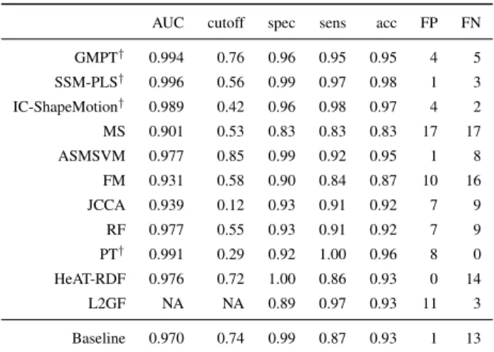
TABLE III
CLASSIFICATION PERFORMANCE RESULTS. THE POSITIVE VALUES WERE
MISHAPES,WHILE THE NEGATIVE VALUES WEREAVSHAPES. NA
DENOTES NOT AVAILABLE VALUE.† DENOTES A METHOD THAT THEAUC
IS STATISTICALLY HIGHER THAN THEBASELINE ATp < 0.05.
AUC cutoff spec sens acc FP FN
GMPT† 0.994 0.76 0.96 0.95 0.95 4 5 SSM-PLS† 0.996 0.56 0.99 0.97 0.98 1 3 IC-ShapeMotion† 0.989 0.42 0.96 0.98 0.97 4 2 MS 0.901 0.53 0.83 0.83 0.83 17 17 ASMSVM 0.977 0.85 0.99 0.92 0.95 1 8 FM 0.931 0.58 0.90 0.84 0.87 10 16 JCCA 0.939 0.12 0.93 0.91 0.92 7 9 RF 0.977 0.55 0.93 0.91 0.92 7 9 PT† 0.991 0.29 0.92 1.00 0.96 8 0 HeAT-RDF 0.976 0.72 1.00 0.86 0.93 0 14 L2GF NA NA 0.89 0.97 0.93 11 3 Baseline 0.970 0.74 0.99 0.87 0.93 1 13
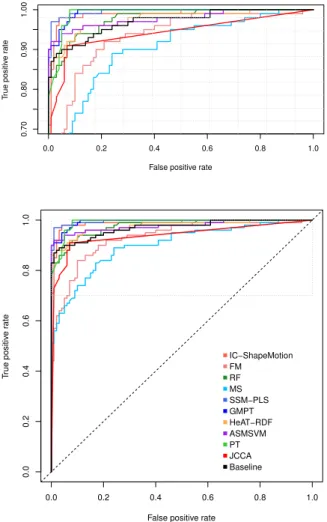
curves (AUC) were above 0.90, which can be confirmed by the ROC curves in Fig. 8. AUC values from four methods: GMPT, SSM-PLS, IC-ShapeMotion and PT were statistically higher than the Baseline (p < 0.05). SSM-PLS achieved the highest accuracy with only four misclassifications. Only SSM-PLS and ASMSVM outperformed the Baseline in all perfor-mance measurements at the optimal cut-off value. The highest sensitivity was achieved by PT without any misclassified MI shapes, while HeAT-RDF did not misclassify AV shapes but 13 MI shapes were incorrectly detected. Note that the Baseline model achieved accuracy of 0.93, but the sensitivity of the model is only 0.87 (with 13 FN and 1 FP).
Figure 8 visually compares the participating methods with the Baseline model (shown as a black curve). The performance of FM and MS were all under the Baseline throughout the range of cut-off values. The optimal cut-off value for method JCCA is slightly above the Baseline ROC curve, but the area under the JCCA ROC curve was lower than the Baseline. The ROC curves of SSM-PLS, IC-ShapeMotion, ASMSVM, PT and GMPT were generally above the Baseline curve, indicating some benefits of shape information for predicting MI. The performance of two random forest classifiers (HeAT-RDF and RF) were similar with the Baseline.
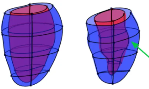
Figure 9 shows the frequency of misclassified cases by the participating methods. The total number of distinct mis-classified cases was 72, where 35 of them (48.6%) were false negatives (MI shapes were misclassified as AV). At least seven methods and also the Baseline model failed to predict two cases, which were both MI shapes. These two difficult cases are shown in Fig. 10. Both cases have cardiac volume and function within the normal range, but detailed geometrical shape visualization shows reduced contraction in local area (pointed by green arrows). GMPT and L2GF methods correctly identified the case of Fig. 10(a), while SSM-PLS and HeAT-RDF correctly identified Fig. 10(b). Only IC-ShapeMotion and PT methods classified both cases correctly.
False positive rate T rue positiv e r ate 0.0 0.2 0.4 0.6 0.8 1.0 0.70 0.80 0.90 1.00
False positive rate
T rue positiv e r ate 0.0 0.2 0.4 0.6 0.8 1.0 0.0 0.2 0.4 0.6 0.8 1.0 IC−ShapeMotion FM RF MS SSM−PLS GMPT HeAT−RDF ASMSVM PT JCCA Baseline
Fig. 8. ROC curves of the participating methods. True positive rate is equal with sensitivity, while false positive rate is (1 - specificity). Top figure enlarges the top part of the ROC space (marked by dotted grey rectangle).
V. DISCUSSION
This challenge provides an open benchmark for testing statistical shape characterization methods describing remod-eling after MI. Although identification of MI by shape alone would not be used clinically (since stress, scar and perfusion imaging [64], [65] are used for this purpose), the classification metrics used in this paper help rank methods in terms of their ability to characterize shape remodeling. One clinical application of these methods would be to track and score patients against a reference population, enabling precise quan-tification of disease severity and effect of treatment. Infarct expansion increases the wall stress and decreased myocardial contraction forces physiological changes in the LV shape and function to maintain sufficient blood supply throughout the circulation [4]–[7]. This is particularly demonstrated by the ventricular enlargement in terms of increased volume and mass [9]. Increased ESV is commonly seen in patients after MI [66] and when prolonged the LV shape becomes more spherical [66]. Hence, the Baseline prediction model,
Fig. 9. Histogram of misclassified cases. False negatives, i.e. MI shapes that were mistakenly identified as AV, are shown to evaluate the sensitivities of the participating methods to identify MI shapes.
which used only EDV, ESV, LVM and EF, could identify MI patients with good accuracy (acc: 0.93, sens: 0.87, spec: 0.99). However, this model was not able to correctly identify all MI patients.
A. Outperforming methods
From 14 misclassified cases from the Baseline method, at least 2 participating methods identified them correctly. This shows that shape information can increase the accuracy of MI characterization compared to the Baseline. In fact, five methods had higher accuracies than the Baseline: GMPT, SSM-PLS, IC-ShapeMotion, ASMSVM and PT. Four of these methods contained common elements, i.e. a traditional statis-tical shape analysis [57], where shape preserving transforma-tions (isotropic scale, rotation and translation) were removed using Procustes alignment. The feature set was subsequently extracted by PCA. This algorithm, which has been made popular by the Active Shape Model for image segmenta-tion [67], turned out to be the best approach to outperform the Baseline model for classifying shapes. The only other alternative approach that had higher accuracy than the Baseline was PT, which used the combination of wall thickness and motion deformation derived from a polyaffine motion model. The ASMSVM method applied the most simple approach of statistical shape analysis by using principal component coefficients as inputs for the SVM. However, this was already sufficient to outperform the Baseline at the optimal cut-off value (see Table III). The GMPT method added Euclidean parallel transport before PCA and its result was also higher than the Baseline. A more effective approach was demon-strated by the SSM-PLS. Instead of aligning feature axes based on geometrical variations in the surface point distribution, it estimated the axes of shape variation that correlated most with the MI classification. SSM-PLS features were therefore clinically meaningful variations optimized for MI prediction, which resulted in only four misclassifications (1 FP and 3 FN). A useful trick to improve performance was to run the method
using several different hidden variables, and then choose the most common result.
All methods used the provided training set to develop a pre-diction model. The JCCA method investigated both supervised and unsupervised approaches and found that the supervised training accuracy was better [42].
Support vector machine was the most popular classifier. However, this does not mean that their classification results were similar. As shown in Fig. 9, most misclassified cases were produced by only one or two methods, indicating large variations in the classification processes. The differences be-tween these methods were in the feature space definition and feature extraction methods.
B. What are the best features for LV shapes?
Features used by the participating methods in this challenge can be grouped into three types: point, shape and displacement features. The point-based feature was determined from the spatial distribution of surface 3D points. The shape features were derived from the LV shape geometry, such as volume, mass, wall thickness and sphericity. The displacement feature is a functional measure between ED and ES shapes, including ejection fraction, wall thickening and surface displacement.
Point-based feature was the most popular type of feature set, which was used by seven methods. Three of them: GMPT, IC-ShapeMotion and ASMSVM used the same feature extraction approach on the surface point set for the same SVM classifier. ASMSVM used only PCA on the point set distributions and achieved 0.95 accuracy. GMPT added parallel transport and it achieved the same accuracy level. IC-ShapeMotion added absolute wall thickness, circumferential displacement of endocardium and radial displacement of epicardium, which increased the accuracy to 0.97.
Adding displacement features appeared to be beneficial for MI shape characterization, as was shown by the IC-ShapeMotion and PT methods. The PT method also included wall thickness feature, which was combined with a set of affine transformations. Both PT and IC-ShapeMotion performance values were higher than the Baseline and both were able to identify the two difficult cases in Fig. 10 correctly. Further-more, the PT method correctly detected all MI shapes, but eight AV shapes were mistakenly identified as MI.
Shape based features produced mixing results. Wall thick-ness defined as radius values in the medial surface (MS) pro-duced lower accuracy than the Baseline, while absolute wall thickness improved the performance in PT. More complicated feature extractions, such as the two-layer generative model of JCCA and surface distortion map of FM, did not demonstrate better performance than the Baseline.
The L2GF method was the only participant that incorporated regional features. A local feature to detect MI shapes is based on the fact that infarction starts locally. Although both were equally accurate, L2GF was more sensitive than the Baseline to detect MI shapes.
C. Are random forests helpful?
Two methods used a random forest classifier: RF and HeAT-RDF. The RF used EDV, ESV and 70 other features,
(a) EDV=109ml, ESV=37ml, LVM=103g, EF=66%
(b) EDV=127ml, ESV=50ml, LVM=116g, EF=61%
Fig. 10. The two most difficult cases where the Baseline and seven
participating methods failed to correctly classify them. Both cases are MI. The left figures show ED shapes, while the right are ES shapes. The green arrows point to less contractile area of the myocardium, indicating infarction.
while HeAT-RDF used 10 features including EDV, ESV and EF. With such rich feature sets, it was expected that these methods would perform better than the Baseline. However, their performance was similar (see their ROC curves in Fig. 8), indicating that this bag of features did not give additional benefit. Other methods, such as GMPT and PT, also considered the random forest classifier during training, but the classifier did not produce the best results.
This challenge problem may not be suitable for the random forest classifier, due to the difficulty in selection of good fea-tures. Both RF and HeAT-RDF have achieved good accuracies (0.92 and 0.93), but random forests suffer if there are too few good variables relative to noisy ones [50]. EDV, ESV and EF are already good features in the Baseline model. Therefore adding too many variables to the random forest appears to be counter-productive.
D. Limitations
There are some limitations in this current challenge. Only ED and ES frames were given in the dataset, but as shown by IC-ShapeMotion and PT methods, incorporating motion infor-mation from other remaining cardiac frames may increase the classification performance. In this challenge, the distributions of risk factors and cardiac function parameters between the two groups were already well separated, which yielded high classification performance by the Baseline prediction model. Quantification of the effects of risk factors and demographics
on remodelling requires a large scale epidemiology study (for example, as is currently being performed in the UK Biobank [68]). Such large scale studies will benefit greatly from the methods evaluated in this study. A more difficult dataset with less separated shape differences may provide more insight into how statistical shape modeling can assist clinical diagnosis. The metric used in this challenge was to automati-cally identify myocardial infarction shapes from asymptomatic volunteers. However, this study does not demonstrate that the methods are able to detect myocardial infarction among other pathological groups. Hence, shape features should be trained on datasets that can control for these confounding factors, before clinical application. Further studies are also needed to investigate different metrics for the quantification of the degree of disease, quantification of regional wall motion abnormalities, predicting the location of scar, or characterizing infarction types (hibernating, remote or stunned).
VI. CONCLUSIONS
This challenge was the first to examine statistical shape analysis methods in the domain of cardiac disease (specifically myocardial infarction). The challenge attracted relatively high community participation and covered a wide range of different approaches, both in statistical analysis and design of shape features. This reflected the variety of approaches being actively investigated by the community at the present time. We believe that the current challenge provides a number of benefits to the community, specifically:
(i) many methods demonstrated that they can be immediately applied in clinical practice to quantify of the degree of adverse remodelling against population norms, and monitor and evaluate patients with myocardial infarction, (ii) specific aspects of some methods have been identified
which would benefit future applications,
(iii) specific shape features have been identified which best describe adverse remodeling of the left ventricle after myocardial infarction.
All the participating methods achieved high accuracy, sen-sitivity and specificity. Although many methods fell short of the Baseline performance, all cases misclassified by the Baseline could be correctly classified by some of the partici-pating methods. Hence, this study demonstrates that statistical shape methods can add information to the understanding of LV remodeling. Shape feature extraction, solely based on geometric morphometric analysis, can outperform traditional clinical measures. Adding motion information increases the performance of these methods. This resource provides a valuable mechanism to benchmark additional algorithms for characterization of myocardial infarction in the future.
REFERENCES
[1] O. Gjesdal, D. A. Bluemke, and J. A. Lima, “Cardiac remodeling at the population level–risk factors, screening, and outcomes,” Nat Rev Cardiol, vol. 8, no. 12, pp. 673–85, Dec 2011.
[2] K. Kallaras, E. A. Sparks, D. P. Schuster, K. Osei, C. F. Wooley, and H. Boudoulas, “Cardiovascular effects of aging. Interrelationships of aortic, left ventricular, and left atrial function,” Herz, vol. 26, no. 2, pp. 129–39, Mar 2001.
[3] C. Mihl, W. R. M. Dassen, and H. Kuipers, “Cardiac remodelling: con-centric versus eccon-centric hypertrophy in strength and endurance athletes,” Neth Heart J, vol. 16, no. 4, pp. 129–33, Apr 2008.
[4] R. M. Norris, “Progressive left ventricular dysfunction and remodeling after myocardial infarction,” Circulation, vol. 89, no. 4, p. 1905, Apr 1994.
[5] Z. R. Yousef, S. R. Redwood, and M. S. Marber, “Postinfarction left ventricular remodeling: a pathophysiological and therapeutic review,” Cardiovasc Drugs Ther, vol. 14, no. 3, pp. 243–52, Jun 2000. [6] M. G. Sutton and N. Sharpe, “Left ventricular remodeling after
my-ocardial infarction: pathophysiology and therapy,” Circulation, vol. 101, no. 25, pp. 2981–8, Jun 2000.
[7] M. A. Konstam, D. G. Kramer, A. R. Patel, M. S. Maron, and J. E. Udelson, “Left ventricular remodeling in heart failure: current concepts in clinical significance and assessment,” JACC Cardiovasc Imaging, vol. 4, no. 1, pp. 98–108, Jan 2011.
[8] P. C. Westman, M. J. Lipinski, D. Luger, R. Waksman, R. O. Bonow, E. Wu, and S. E. Epstein, “Inflammation as a Driver of Adverse Left Ventricular Remodeling After Acute Myocardial Infarction,” J Am Coll Cardiol, vol. 67, no. 17, pp. 2050–60, May 2016.
[9] E. Wu, J. T. Ortiz, P. Tejedor, D. C. Lee, C. Bucciarelli-Ducci, P. Kansal, J. C. Carr, T. A. Holly, D. Lloyd-Jones, F. J. Klocke, and R. O. Bonow, “Infarct size by contrast enhanced cardiac magnetic resonance is a stronger predictor of outcomes than left ventricular ejection fraction or end-systolic volume index: prospective cohort study,” Heart, vol. 94, no. 6, pp. 730–6, Jun 2008.
[10] L. H. Baur, J. J. Schipperheyn, E. E. van der Wall, J. H. Reiber, A. D. van Dijk, C. Brobbel, J. J. Kerkkamp, P. J. Voogd, and A. V. Bruschke, “Regional myocardial shape alterations in patients with anterior my-ocardial infarction,” Int J Card Imaging, vol. 12, no. 2, pp. 89–96, Jun 1996.
[11] N. D’Elia, J. D’hooge, and T. H. Marwick, “Association Between My-ocardial Mechanics and Ischemic LV Remodeling,” JACC Cardiovasc Imaging, vol. 8, no. 12, pp. 1430–43, Dec 2015.
[12] J. N. Cohn, R. Ferrari, and N. Sharpe, “Cardiac remodeling–concepts and clinical implications: a consensus paper from an international forum on cardiac remodeling. Behalf of an International Forum on Cardiac Remodeling,” J Am Coll Cardiol, vol. 35, no. 3, pp. 569–82, Mar 2000. [13] S. P. Wong, J. K. French, A.-M. Lydon, S. O. M. Manda, W. Gao, N. G. Ashton, and H. D. White, “Relation of left ventricular sphericity to 10-year survival after acute myocardial infarction,” Am J Cardiol, vol. 94, no. 10, pp. 1270–5, Nov 2004.
[14] M. Cirillo, A. Amaducci, F. Brunelli, M. Dalla Tomba, P. Parrella, G. Tasca, G. Troise, and E. Quaini, “Determinants of postinfarction remodeling affect outcome and left ventricular geometry after surgical treatment of ischemic cardiomyopathys,” J Thorac Cardiovasc Surg, vol. 127, no. 6, pp. 1648–56, Jun 2004.
[15] J. Schulz-Menger, D. A. Bluemke, J. Bremerich, S. D. Flamm, M. A. Fogel, M. G. Friedrich, R. J. Kim, F. von Knobelsdorff-Brenkenhoff, C. M. Kramer, D. J. Pennell, S. Plein, and E. Nagel, “Standardized image interpretation and post processing in cardiovascular magnetic resonance: Society for Cardiovascular Magnetic Resonance (SCMR) board of trustees task force on standardized post processing,” J Cardiovasc Magn Reson, vol. 15, p. 35, 2013.
[16] S. G. Myerson, N. G. Bellenger, and D. J. Pennell, “Assessment of left ventricular mass by cardiovascular magnetic resonance,” Hypertension, vol. 39, no. 3, pp. 750–5, Mar 2002.
[17] O. Camara, T. Mansi, M. Pop, K. S. Rhode, M. Sermesant, and A. A. Young, Eds., Statistical Atlases and Computational Models of the Heart. Imaging and Modelling Challenges - 6th International Workshop, STACOM 2015, Revised Selected Papers, ser. Lecture Notes in Computer Science, vol. 9534. Springer, 2016.
[18] J. L. Bruse, E. Cervi, K. McLeod, G. Biglino, M. Sermesant, X. Pennec, A. M. Taylor, S. Schievano, T.-Y. Hsia, A. Taylor, S. Khambadkone, M. de Leval, T. Y. Hsia, E. Bove, A. Dorfman, G. H. Baker, A. Hlavacek, F. Migliavacca, G. Pennati, G. Dubini, A. Marsden, I. Vignon-Clementel, and R. Figliola, “Looks Do Matter! Aortic Arch Shape After Hypoplastic Left Heart Syndrome Palliation Correlates With Cavopulmonary Outcomes,” in The Fifty-second Annual Meeting
of The Society of Thoracic Surgeons. Elsevier, 2016/12/04 2016.
[Online]. Available: http://dx.doi.org/10.1016/j.athoracsur.2016.06.041 [19] A. Suinesiaputra, P. Medrano-Gracia, B. R. Cowan, and A. A. Young,
“Big heart data: advancing health informatics through data sharing in cardiovascular imaging,” IEEE J Biomed Health Inform, vol. 19, no. 4, pp. 1283–90, Jul 2015.
[20] X. Zhang, B. R. Cowan, D. A. Bluemke, J. P. Finn, C. G. Fonseca, A. H. Kadish, D. C. Lee, J. A. C. Lima, A. Suinesiaputra, A. A. Young, and Final version of this paper available at http://ieeexplore.ieee.org/
P. Medrano-Gracia, “Atlas-based quantification of cardiac remodeling due to myocardial infarction,” PLoS One, vol. 9, no. 10, p. e110243, 2014.
[21] S. Ardekani, S. Jain, A. Sanzi, C. P. Corona-Villalobos, T. P. Abraham, M. R. Abraham, S. L. Zimmerman, K. C. Wu, R. L. Winslow, M. I. Miller, and L. Younes, “Shape analysis of hypertrophic and hypertensive heart disease using MRI-based 3D surface models of left ventricular geometry,” Med Image Anal, vol. 29, pp. 12–23, Apr 2016.
[22] H. Zhang, A. Wahle, R. K. Johnson, T. D. Scholz, and M. Sonka, “4-D cardiac MR image analysis: left and right ventricular morphology and function,” IEEE Trans Med Imaging, vol. 29, no. 2, pp. 350–64, Feb 2010.
[23] P. Piras, A. Evangelista, S. Gabriele, P. Nardinocchi, L. Teresi, C. Tor-romeo, M. Schiariti, V. Varano, and P. E. Puddu, “4D-analysis of left ventricular heart cycle using procrustes motion analysis,” PLoS One, vol. 9, no. 1, p. e86896, 2014.
[24] T. Mansi, I. Voigt, B. Leonardi, X. Pennec, S. Durrleman, M. Sermesant, H. Delingette, A. M. Taylor, Y. Boudjemline, G. Pongiglione, and N. Ayache, “A statistical model for quantification and prediction of cardiac remodelling: application to tetralogy of Fallot,” IEEE Trans Med Imaging, vol. 30, no. 9, pp. 1605–16, Sep 2011.
[25] S. Faghih Roohi and R. Aghaeizadeh Zoroofi, “4D statistical shape modeling of the left ventricle in cardiac MR images,” Int J Comput Assist Radiol Surg, vol. 8, no. 3, pp. 335–51, May 2013.
[26] W. Bai, W. Shi, A. de Marvao, T. J. W. Dawes, D. P. O’Regan, S. A. Cook, and D. Rueckert, “A bi-ventricular cardiac atlas built from 1000+ high resolution MR images of healthy subjects and an analysis of shape and motion,” Med Image Anal, vol. 26, no. 1, pp. 133–45, Dec 2015. [27] C. Hoogendoorn, N. Duchateau, D. S´anchez-Quintana, T. Whitmarsh,
F. M. Sukno, M. De Craene, K. Lekadir, and A. F. Frangi, “A high-resolution atlas and statistical model of the human heart from multislice CT,” IEEE Trans Med Imaging, vol. 32, no. 1, pp. 28–44, Jan 2013. [28] P. Medrano-Gracia, B. R. Cowan, B. Ambale-Venkatesh, D. A. Bluemke,
J. Eng, J. P. Finn, C. G. Fonseca, J. A. C. Lima, A. Suinesiaputra, and A. A. Young, “Left ventricular shape variation in asymptomatic populations: the Multi-Ethnic Study of Atherosclerosis,” J Cardiovasc Magn Reson, vol. 16, p. 56, 2014.
[29] E. Bardinet, L. D. Cohen, and N. Ayache, “A parametric deformable model to fit unstructured 3D data,” Computer vision and image under-standing, vol. 71, no. 1, pp. 39–54, 1998.
[30] A. B. Abdallah, F. Ghorbel, K. Chatti, H. Essabbah, and M. H. Bedoui, “A new uniform parameterization and invariant 3D spherical harmonic shape descriptors for shape analysis of the heart’s left ventricle–A pilot study,” Pattern Recognition Letters, vol. 31, no. 13, pp. 1981–1990, 2010.
[31] Y. Yu, S. Zhang, K. Li, D. Metaxas, and L. Axel, “Deformable models with sparsity constraints for cardiac motion analysis,” Med Image Anal, vol. 18, no. 6, pp. 927–37, Aug 2014.
[32] A. F. Frangi, W. J. Niessen, and M. A. Viergever, “Three-dimensional modeling for functional analysis of cardiac images: a review,” IEEE Trans Med Imaging, vol. 20, no. 1, pp. 2–25, Jan 2001.
[33] A. H. Kadish, D. Bello, J. P. Finn, R. O. Bonow, A. Schaechter, H. Subacius, C. Albert, J. P. Daubert, C. G. Fonseca, and J. J. Goldberger, “Rationale and design for the Defibrillators to Reduce Risk by Magnetic Resonance Imaging Evaluation (DETERMINE) trial,” J Cardiovasc Electrophysiol, vol. 20, no. 9, pp. 982–7, Sep 2009. [34] D. E. Bild, D. A. Bluemke, G. L. Burke, R. Detrano, A. V. Diez Roux,
A. R. Folsom, P. Greenland, D. R. Jacob, Jr, R. Kronmal, K. Liu, J. C. Nelson, D. O’Leary, M. F. Saad, S. Shea, M. Szklo, and R. P. Tracy, “Multi-Ethnic Study of Atherosclerosis: objectives and design,” Am J Epidemiol, vol. 156, no. 9, pp. 871–81, Nov 2002.
[35] C. G. Fonseca, M. Backhaus, D. A. Bluemke, R. D. Britten, J. D. Chung, B. R. Cowan, I. D. Dinov, J. P. Finn, P. J. Hunter, A. H. Kadish, D. C. Lee, J. A. C. Lima, P. Medrano-Gracia, K. Shivkumar, A. Suinesiaputra, W. Tao, and A. A. Young, “The Cardiac Atlas Project–an imaging database for computational modeling and statistical atlases of the heart,” Bioinformatics, vol. 27, no. 16, pp. 2288–95, Aug 2011.
[36] P. Piras, L. Teresi, S. Gabriele, A. Evangelista, G. Esposito, V. Varano, C. Torromeo, P. Nardinocchi, and P. E. Puddu, “Systo-Diastolic LV Shape Analysis by Geometric Morphometrics and Parallel Transport Highly Discriminates Myocardial Infarction,” in Statistical Atlases and Computational Models of the Heart. Imaging and Modelling Challenges - 6th International Workshop, STACOM 2015, Revised Selected Papers, ser. Lecture Notes in Computer Science, O. Camara, T. Mansi, M. Pop, K. S. Rhode, M. Sermesant, and A. A. Young, Eds., vol. 9534. Springer, 2016, pp. 119–129.
[37] K. Lekadir, X. Alb`a, M. Perea˜nez, and A. F. Frangi, “Statistical Shape Modeling Using Partial Least Squares: Application to the Assessment of Myocardial Infarction,” in Statistical Atlases and Computational Models of the Heart. Imaging and Modelling Challenges - 6th International Workshop, STACOM 2015, Revised Selected Papers, ser. Lecture Notes in Computer Science, O. Camara, T. Mansi, M. Pop, K. S. Rhode,
M. Sermesant, and A. A. Young, Eds., vol. 9534. Springer, 2016,
pp. 130–139.
[38] W. Bai, O. Oktay, and D. Rueckert, “Classification of Myocardial Infarcted Patients by Combining Shape and Motion Features,” in Sta-tistical Atlases and Computational Models of the Heart. Imaging and Modelling Challenges - 6th International Workshop, STACOM 2015, Revised Selected Papers, ser. Lecture Notes in Computer Science, O. Camara, T. Mansi, M. Pop, K. S. Rhode, M. Sermesant, and A. A. Young, Eds., vol. 9534. Springer, 2016, pp. 140–145.
[39] P. Ablin and K. Siddiqi, “Detecting Myocardial Infarction Using Medial Surfaces,” in Statistical Atlases and Computational Models of the Heart. Imaging and Modelling Challenges - 6th International Workshop, STACOM 2015, Revised Selected Papers, ser. Lecture Notes in Computer Science, O. Camara, T. Mansi, M. Pop, K. S. Rhode, M. Sermesant, and A. A. Young, Eds., vol. 9534. Springer, 2016, pp. 146–153. [40] N. Parajuli, A. Lu, and J. S. Duncan, “Left Ventricle Classification Using
Active Shape Model and Support Vector Machine,” in Statistical Atlases and Computational Models of the Heart. Imaging and Modelling Chal-lenges - 6th International Workshop, STACOM 2015, Revised Selected Papers, ser. Lecture Notes in Computer Science, O. Camara, T. Mansi, M. Pop, K. S. Rhode, M. Sermesant, and A. A. Young, Eds., vol. 9534. Springer, 2016, pp. 154–161.
[41] A. Mukhopadhyay, I. Oksuz, and S. A. Tsaftaris, “Supervised Learning of Functional Maps for Infarct Classification,” in Statistical Atlases and Computational Models of the Heart. Imaging and Modelling Challenges - 6th International Workshop, STACOM 2015, Revised Selected Papers, ser. Lecture Notes in Computer Science, O. Camara, T. Mansi, M. Pop, K. S. Rhode, M. Sermesant, and A. A. Young, Eds., vol. 9534. Springer, 2016, pp. 162–170.
[42] C. Pinto, S. C¸imen, A. Gooya, K. Lekadir, and A. F. Frangi, “Joint Clustering and Component Analysis of Spatio-Temporal Shape Patterns in Myocardial Infarction,” in Statistical Atlases and Computational Mod-els of the Heart. Imaging and Modelling Challenges - 6th International Workshop, STACOM 2015, Revised Selected Papers, ser. Lecture Notes in Computer Science, O. Camara, T. Mansi, M. Pop, K. S. Rhode,
M. Sermesant, and A. A. Young, Eds., vol. 9534. Springer, 2016,
pp. 171–179.
[43] J. Allen, E. Zacur, E. Dall’Armellina, P. Lamata, and V. Grau, “My-ocardial Infarction Detection from Left Ventricular Shapes Using a Random Forest,” in Statistical Atlases and Computational Models of the Heart. Imaging and Modelling Challenges - 6th International Workshop, STACOM 2015, Revised Selected Papers, ser. Lecture Notes in Computer Science, O. Camara, T. Mansi, M. Pop, K. S. Rhode, M. Sermesant, and A. A. Young, Eds., vol. 9534. Springer, 2016, pp. 180–189. [44] M.-M. Roh´e, N. Duchateau, M. Sermesant, and X. Pennec,
“Com-bination of Polyaffine Transformations and Supervised Learning for the Automatic Diagnosis of LV Infarct,” in Statistical Atlases and Computational Models of the Heart. Imaging and Modelling Challenges - 6th International Workshop, STACOM 2015, Revised Selected Papers, ser. Lecture Notes in Computer Science, O. Camara, T. Mansi, M. Pop, K. S. Rhode, M. Sermesant, and A. A. Young, Eds., vol. 9534. Springer, 2016, pp. 190–198.
[45] J. Ehrhardt, M. Wilms, H. Handels, and D. S¨aring, “Automatic Detection of Cardiac Remodeling Using Global and Local Clinical Measures and Random Forest Classification,” in Statistical Atlases and Computational Models of the Heart. Imaging and Modelling Challenges - 6th Interna-tional Workshop, STACOM 2015, Revised Selected Papers, ser. Lecture Notes in Computer Science, O. Camara, T. Mansi, M. Pop, K. S. Rhode, M. Sermesant, and A. A. Young, Eds., vol. 9534. Springer, 2016, pp. 199–207.
[46] M. Tabassian, M. Alessandrini, P. Claes, L. Marchi, D. Vandermeulen, G. Masetti, and J. D’hooge, “Automatic Detection of Myocardial In-farction Through a Global Shape Feature Based on Local Statistical Modeling,” in Statistical Atlases and Computational Models of the Heart. Imaging and Modelling Challenges - 6th International Workshop, STACOM 2015, Revised Selected Papers, ser. Lecture Notes in Computer Science, O. Camara, T. Mansi, M. Pop, K. S. Rhode, M. Sermesant, and A. A. Young, Eds., vol. 9534. Springer, 2016, pp. 208–216. [47] P. M. Nielsen, I. J. Le Grice, B. H. Smaill, and P. J. Hunter,
“Math-ematical model of geometry and fibrous structure of the heart,” Am J Physiol, vol. 260, no. 4 Pt 2, pp. H1365–78, Apr 1991.