Measurement of Sound Transmission from Meeting Rooms

(1)

Publisher’s version / Version de l'éditeur:

Vous avez des questions? Nous pouvons vous aider. Pour communiquer directement avec un auteur, consultez la

première page de la revue dans laquelle son article a été publié afin de trouver ses coordonnées. Si vous n’arrivez

Questions? Contact the NRC Publications Archive team at

PublicationsArchive-ArchivesPublications@nrc-cnrc.gc.ca. If you wish to email the authors directly, please see the first page of the publication for their contact information.

https://publications-cnrc.canada.ca/fra/droits

L’accès à ce site Web et l’utilisation de son contenu sont assujettis aux conditions présentées dans le site LISEZ CES CONDITIONS ATTENTIVEMENT AVANT D’UTILISER CE SITE WEB.

Research Report (National Research Council of Canada. Institute for Research in Construction), 2006-03-01

READ THESE TERMS AND CONDITIONS CAREFULLY BEFORE USING THIS WEBSITE.

https://nrc-publications.canada.ca/eng/copyright

NRC Publications Archive Record / Notice des Archives des publications du CNRC :

https://nrc-publications.canada.ca/eng/view/object/?id=76c9d48e-384d-4131-94f2-b60937dea923 https://publications-cnrc.canada.ca/fra/voir/objet/?id=76c9d48e-384d-4131-94f2-b60937dea923

NRC Publications Archive

Archives des publications du CNRC

For the publisher’s version, please access the DOI link below./ Pour consulter la version de l’éditeur, utilisez le lien DOI ci-dessous.

https://doi.org/10.4224/20378338

Access and use of this website and the material on it are subject to the Terms and Conditions set forth at

Measurement of Sound Transmission from Meeting Rooms Bradley, J. S.; Gover, B. N.

(2)

http://irc.nrc-cnrc.gc.ca

M e a sure m e nt of Sound Tra nsm ission

from M e e t ing Room s

I R C - R R - 2 2 0

B r a d l e y , J . S . ; G o v e r , B . N .

(3)

Measurement of Sound Transmission

from Meeting Rooms

John S. Bradley and Bradford N. Gover

IRC Research Report, IRC RR-220

March 2006

(4)

Summary

A meeting room is said to be completely speech secure when persons outside the room are not able to understand conversations from within the room, or in more extreme cases are not able to detect any speech sounds from the room. This report describes

measurements of sound transmission from meeting rooms to adjacent spaces to evaluate procedures for assessing the speech security of the meeting rooms.

The conventional approach of measuring sound isolation between rooms is from the differences in space-average sound levels in each room. This is not valid for many situations where speech security needs to be verified. A new method is proposed and evaluated in which attenuations between room-average sound levels in meeting rooms to spot receiver positions near the outside of these rooms are used to evaluate the speech security of the room. The new method avoids problems with ill-defined receiving spaces, and spaces that do not have even approximately diffuse sound fields. It also provides assessments of speech security for more sensitive locations where an eavesdropper is more likely to be found.

The method first requires the creation of an approximately homogeneous sound field in the meeting room. The new measurements confirm that this can be done more precisely (i.e. lower spatial standard deviations of sound levels in the source room) and more efficiently (i.e. fewer measurements required) using an omni-directional rather than a conventional directional sound source. To define the mean sound levels in the source room, microphones must be located at a number of positions in the source room. When using an omni-directional sound source, about half as many measurement positions are required compared to when using a more conventional directional sound source.

Using an omni-directional sound source also provides a more even distribution of sound on all of the boundaries of the meeting room. The transmission of sound to adjacent spaces will depend on the distribution of sound energy on each surface as well as the distribution of the angles of incidence of the sound on the room boundaries. The less homogeneous sound fields created using a directional source lead to significantly different ratings of speech security at many locations. The often suggested approach of locating directional sources pointing into opposite corners of the room relative to the test wall was also evaluated but produced much less homogeneous sound fields (i.e. larger spatial standard deviations) than when using an omni-directional source. This technique is also less efficient because it requires the source room measurements to be repeated for each test wall of the meeting room.

The results make it possible to provide specific recommendations concerning the details of the proposed new speech security measurement protocol. This includes the numbers of measurements required for four different categories of meeting rooms (defined later in this report) and specifications for the sound source.

Using the new measurement protocol, speech security ratings based on signal-to-noise ratio measures can be determined with some precision at sensitive locations near meeting rooms. These measures have been previously related to subjective ratings of the

(5)

Acknowledgments

This project was jointly funded by Public Works and Government Services Canada (PWGSC), the Royal Canadian Mounted Police (RCMP) and the National Research Council (NRC). PWGSC and RCMP personnel were also instrumental in finding suitable rooms for all of the measurements. In particular the authors would like to thank Don Nixon and Bonnie Belwa (at PWGSC) who because of their considerable efforts made this all happen. The authors would also like to thank Ms. Frances King who helped in the final analyses of the data, and gratefully acknowledge the dedicated efforts of Mr. Darren Ronda who carried out all of the measurements and the initial analyses of the results presented in this report while on an engineering coop work term at NRC.

(6)

Table

of

1. Introduction

This report describes measurements of sound transmission from meeting rooms to adjacent spaces to evaluate new procedures for assessing the speech security of meeting rooms.

A meeting room is said to be completely speech secure when persons outside the room are not able to understand conversations from within the room, or in more extreme cases are not able to detect any speech sounds from the room. The audibility and intelligibility of transmitted speech sounds are related to the level of speech sounds relative to existing ambient noise levels at locations outside the meeting room. The levels of speech sounds from adjacent meeting rooms will depend on the loudness of the speech in the meeting room and the sound transmission characteristics of the room boundaries.

Previous related work has measured speech levels in meeting rooms to provide a

statistical description of the likelihood of various speech levels occurring in meetings [1]. There is a wide range of possible speech levels. Although higher levels are more likely to lead to speech security problems, they are much less likely to occur. Similarly, statistical distributions of ambient noise levels near meeting rooms were determined. The likelihood of various speech levels, and of various ambient noise levels in the adjacent spaces, can be used to estimate the probability of particular combinations of speech and noise levels occurring and hence the risk of a speech security lapse. Of course whether there is a speech security problem for a particular combination of speech and noise level will depend on the sound transmission characteristics from the meeting room to the adjacent space.

Designing to provide adequate speech security for louder but less likely events (usually corresponding to higher speech levels and lower ambient noise levels) will provide a higher degree of speech security, but will require higher and usually more costly sound insulation. This process would be similar to designing a roof to withstand a snow load that might occur only once in a typical 100 year interval. Making the roof stronger (equivalent to higher sound transmission loss) would make it even less likely that snow load would be excessive over the same 100 year period, because the roof would be strong enough to support an even heavier but less likely snow load. However, the need for a stronger roof must be balanced against associated costs and other practical concerns. To determine whether some combination of transmitted speech level and ambient noise level will lead to a speech security problem, other previous related work [2,3] has developed signal-to-noise ratio measures that can be used to assess the audibility and/or intelligibility of the transmitted speech sounds. These signal-to-noise ratio measures compare the level of the transmitted speech (i.e. the ‘signal’) at various frequencies to the ambient noise levels (the ‘noise’) over the same range of frequencies. The previous work also determined the thresholds: of the audibility of speech sounds, of the audibility of the cadence of speech, and of the intelligibility of speech in terms of these new signal-to-noise ratio measures.

Given some unlikely high speech level and similarly unlikely low ambient noise level, one could first estimate or measure the expected transmitted speech levels. Combining the transmitted speech levels with ambient noise levels, one can then calculate whether the meeting room will be speech secure in terms of the new signal-to-noise ratio

(8)

measures. Of course, this requires knowledge of the sound transmission characteristics of the room boundaries. This report considers the merits and accuracy of various approaches for measuring the sound transmission characteristics of meeting room boundaries related to the needs of assessing the speech security of meeting rooms.

A new measurement procedure is proposed that measures sound transmission from

meeting rooms to points just outside the room. This is compared to the more conventional approach of measuring sound transmission between room-average measurements in both spaces. The measurements are also used to evaluate the benefits of using an

omni-directional sound source, and to determine how the accuracy of the sound transmission characteristics is influenced by the number of measurement positions.

In order make this report more readable, the details of various calculations and measurement results are included in appendices. This is intended to provide a more concise but complete description of the work in the various chapters of the main report. Chapter 2 gives a short description of the proposed new measurement procedure. This is followed by the details of the various measurements carried out in Chapter 3. The eleven meeting rooms that were included in these measurements are described in Chapter 4. Chapters 5 and 6 provide the main results of this work. In Chapter 5, the analyses of measurements of room average sound levels in the source rooms are presented. In Chapter 6 the analyses of sound transmission measurements from room average levels to spot measurement positions are discussed. Chapter 7 discusses the implications of the results for various details of the proposed new measurement procedure. The final chapter provides some overall conclusions from the work.

(9)

2. The Proposed New Procedure

The sound transmission characteristics of room boundaries are usually measured in terms of room-average sound levels in the source and receiving room. For example, the ASTM standard E336 describes such a measurement procedure to evaluate airborne sound transmission between an adjacent pair of rooms. According to such standards, the sound transmission loss of the room boundary (TL(f)) is measured as a function of frequency using the following relationship,

TL(f) = LS(f) – LR(f) +10 log{S/A(f)}, dB (1)

where, LS(f) is the room-average source room sound level,

LR(f) is the room-average receiving room sound level,

S is the area of the common boundary between the two rooms, m2,

A(f) is the total sound absorption in the receiving space in m2.

By rearranging this equation one can predict expected mean levels in the receiving space if the other parameters are known.

LR(f) = LS(f) – TL(f) +10 log{S/A(f)}, dB (2)

This equation is derived assuming that the sound fields in both rooms are ideally diffuse. That is, sound levels are assumed to be homogenous throughout each room and sound is incident on the common boundary equally from all directions.

Many meeting rooms may be considered to have approximately diffuse sound fields. However, the more irregular their shape and the larger the amount of sound absorbing material in a room, the less they will approximate diffuse field conditions. Although many meeting rooms may have approximately diffuse sound fields, the spaces next to them, where an eavesdropper might be located, could vary from broom closets to large irregular spaces such as hallways or open-plan office areas. Many adjacent spaces will not have diffuse sound fields and equation (1) and (2) would not be valid.

A second problem is that these equations can only be used to predict room-average speech levels in the receiving space. However, listening from some average position in the middle of the room would not be the most sensitive location for overhearing

conversations from the meeting room. Clearly anyone seriously attempting to eavesdrop would be located close to the room boundaries and not in the middle of the receiving room.

The proposed new method is intended to avoid invalid assumptions of diffuse sound fields and to predict transmitted speech levels at more sensitive locations where an eavesdropper might logically be located. First, it is assumed that the talker could be anywhere in the meeting room and that the room must be speech secure for all talkers at all locations in the meeting room. Second, it is assumed that speech security must be obtained for potential eavesdroppers at more sensitive listening locations close to the outside boundaries of the room. Therefore the new method assesses the transmission of speech sounds from room-average levels in the meeting room (the source room) to points 0.25 m from the outside boundary of the meeting room, in adjacent spaces. The required

(10)

transmitted speech levels 0.25 m from the outside boundaries of the meeting room, L0.25

can be determined from the following equation,

L0.25(f) = LS(f) - TL(f) + k, dB (3)

Where k has a value close to 0 dB, and is currently being empirically determined in ongoing work.

This approach makes it possible to predict expected transmitted speech levels without having to assume diffuse field conditions in the receiving space and hence avoids the errors associated with such an assumption. It also makes it possible to predict expected speech levels at the most sensitive locations for any casual eavesdropper.

This method will depend on creating and measuring an ideally homogeneous distribution of sound in the meeting room to be representative of the combined effects of all possible talkers anywhere in the meeting room. The accuracy of the method will depend on how well this is achieved. First the source room-average must be based on a number of source positions distributed throughout the source room. Even though their effect is measured one at a time, the combined average of a large enough number of source positions will represent a homogeneous distribution of sound in the source room. To precisely measure this homogenous distribution of sound, a number of microphone positions distributed throughout the space must be used.

The excitation of the source room must also ensure a good distribution of the incident sound on each boundary of the room. This includes an even distribution of sound energy as well as the angles of incidence of the sound energy on all parts of each room boundary. This report examines the effects of different types and numbers of sound sources on the measurement of the speech security rating of 11 different meeting rooms. It also includes the effect of the number of microphone positions used to characterize conditions in the source room.

The transmitted levels at positions 0.25 m from the outside boundaries of the room will vary from location to location, possibly indicating leaks or weak spots in the sound transmission characteristics of the room boundary. Therefore the locations and numbers of positions must be chosen to describe all potential acoustical problems. These

measurements will describe the unique conditions at each spot measurement position 0.25 m from the outside boundary of the room.

(11)

3. Measurement Details

3.1 Measurement of sound levels in rooms

This section briefly discusses the basic principles of the variation of sound levels in rooms and how one should obtain sufficiently accurate mean sound levels. The mathematical details behind this discussion are included in Appendix 1.

Above a particular frequency, the variations in sound level in a room are random in nature. This frequency is called the Schroeder frequency [4]. The Schroeder frequencies for each room are given in Table A1.2 in Appendix 1. For the consideration of speech sounds, we are mostly concerned about frequencies from 160 to 8,000 Hz. In almost all cases for the meeting rooms that we measured, this frequency range for speech is above the Schroeder frequency. Therefore, we can obtain more precise measurements of the mean values by averaging over a larger number of independent source and receiver positions. To be independent samples of the randomly varying sound levels, source and receiver positions must be separated by at least ½ wavelength at the lowest frequency of interest for speech (160 Hz). This implies a separation of at least 1.2 m. In smaller rooms it may become difficult to have a large enough number of source or receiver positions that fulfill this criteria at the lowest frequency of interest.

Microphone positions must also be sufficiently distant from each source position so that they are in the reverberant field of the source. Close to the source, sound levels decrease with increasing source-to-receiver distance. The point where the direct sound levels have decreased to the point that they are equal to the reverberant sound levels for ideally diffuse conditions is referred to as the critical distance. Further away from the source than the critical distance, sound levels are assumed to not vary systematically with increasing distance in an ideal diffuse field. Although this is not strictly true in most meeting rooms, because the sound fields are not ideally diffuse, the critical distance can easily be

calculated and is a useful minimum value for the distance between source and receiver positions. (The critical distances, when using an omni-directional sound source, for each room are given in Table A1.2 in Appendix 1). When a directional source is used, the critical distance can be considerably larger than for an omni-directional source. Generally this makes it difficult to obtain sufficiently accurate mean sound levels using a

conventional directional loudspeaker source.

When measurements of the source room sound levels are made according to these

criteria, each will be an independent sample of the reverberant sound field in the meeting room. The standard deviation of such measurements is indicative of the spatial variation of sound levels in the source room. Of course, this should include variations of both source and receiver positions. The accuracy of the mean sound levels obtained by averaging these measurements is given by the standard error of the mean value. The standard error of the mean value, SE, is related to the standard deviations of the

distribution of measured levels, σ, and the number of measurements N (as described in equation A1.6 in Appendix 1). We can increase the precision of the mean values by increasing the number of measurements N. Of course, there may be various practical limits on the number of independent measurement positions that can be used, such as the small size of the room.

(12)

It is possible to predict the expected variance of the measured sound levels in a room (as described in Appendix 1). The theoretical variance of sound levels increases with

increasing reverberation time. These theoretical predictions have been calculated and are included for comparison with all measurements of the standard deviations of sound levels in the meeting rooms.

3.2 Description of measurements

Average source room levels were determined using several different methods to compare the benefits of each approach. Measurements were repeated using an omni-directional source (OMNI) or a directional source (DIR) to excite the source room. The OMNI source consisted of 12 four-inch loudspeakers in a dodecahedron shaped enclosure. The DIR source was a Tracoustics noise source that contained one 10 inch driver in a box with the associated power amplifier. The OMNI source was located at up to 6 different positions in the source room at approximately head height (1.5 m) so that the combined effect would be equivalent to homogeneously exciting the room. The DIR source was located on the floor in the 2 corners opposite to each test wall and measurements were repeated for each orientation of the DIR source (pointing into and out of the corner). It is often suggested that pointing directional sources into room corners will reduce the unwanted variations in sound levels due to the directionality of these sources.

For each of the different methods of exciting the source room, transmitted levels were measured at spot-receiver positions 0.25 m from the outside of the meeting room wall under test, and also at positions intended to provide space-average transmitted sound levels in the receiving space. Usually 6 different microphone locations were used to measure receiving space-average levels unless the space was too small for this many independent receiver positions.

Table 3.1 lists the number of source and receiver positions used in the measurements associated with each of the 11 meeting rooms. In the source room (the meeting room), 6 OMNI source positions and 6 receiver (microphone) positions were used unless the room was too small to make this possible. The number of DIR source positions depended on the number of different walls included in the sound transmission measurements. If there was only 1 wall, there are 4 DIR source positions listed in Table 3.1. These corresponded to the combinations of the DIR source located in each of two opposite corners and

oriented both into (DIR-IN) and out of (DIR-OUT) the corners. Table 3.1 also lists the number of spot-receiver positions in adjacent spaces. These correspond to microphones located 0.25 m from the outside of the meeting room. The number of spot receiver positions was determined by the number of different interesting situations that could be found. The last column of Table 3.1 gives the number of microphone positions used to obtain space-average sound levels in the receiving space. This number was again usually 6 but fewer were used in smaller spaces.

From these measurements, attenuations were calculated in 1/3 octave bands, from the

source room-average levels for each source type and orientation, to both individual spot-receiver positions and also to receiving space-average levels. Each set of 1/3 octave band

attenuations was used to calculate 4 different speech security measures. These were 3 different signal-to-noise type measures and the fourth was the predicted transmitted

(13)

A-in many meetA-ings [1] had shown this to be the 98th percentile speech level in meeting rooms. (That is this speech level was only exceeded 2% of the time and 98% of the time the speech level was 69 dBA or less). The signal-to-noise ratio measures were the SII weighted signal-to-noise ratio (SNRSII22), the uniform weighted signal-to-noise ratio

(SNRUNI32), and the simple A-weighted level difference between transmitted speech and

ambient noise levels (ΔdBA). In calculating the signal-to noise ratio measures, a common

ambient noise level of 36 dBA with a –5 dB per octave spectrum shape was used. This would represent a 2nd percentile ambient day-time noise level in spaces near meeting

Table 3.1. N

rooms [1].

umbers of source and receiver positions used, N, for measurements

from the results of listening tests using an

Volume, N, OMNI N, DIR

N, source room N, Spot N, space average Room m3 sources sources* receivers receivers receivers

DT office 56.00 3 4 6 7 6 Com 02 58.01 3 8 4 6 4 MA office 65.84 3 6 4 8 4 Terrace 107.86 3 4 4 6 4 Com 10 206.82 6 8 6 10 6 M20 R114 225.67 6 4 6 12 6 RCMP 229.50 4 6 6 6 6 Colonel By 233.28 6 4 6 10 6 Papineau 379.23 6 4 6 4 6 Health Canada 512.73 6 8 6 12 6 Centennial 518.48 6 4 6 8 6

* includes both DIR-IN and DIR-OUT orientations as different positions

associated with each of the 11 meeting rooms.

3.3 Signal-to-noise ratio measures

Signal-to-noise ratio measures were derived

approach that is similar to some of the steps involved in computing the Articulation Index, AI, or the Speech Intelligibility Index, SII [2,3]. The signal-to-noise ratio in each frequency band, expressed in decibels, is first determined and then a weighted sum across all 1/3 octave bands is performed. The expression for the resulting weighted

signal-to-noise ratioSNR_w_,_dB is

∑

× − = b b b b dB w w LS LN dB SNR _, [ ], (1)

where LSb is the speech level in frequency band LNb is the noise level in band and

T

ere ,

b b,

b

w are the frequency weightings. The weights w reflect the importance of the speech-to-_b

se level difference in each frequency band b he subscript ‘

noi . dB’ in SNRw,dB indicates

the level below which very small 1/3 octave band speech-to-noise level diff nces were

clipped to avoid undetectable low values from influencing the calculated SNRw,dB value.

The signal-to-noise ratio measure SNRSII22, obtained using the frequency weightings from

the ANSI S3.5 standard for the Speech Intelligibility Index measure, was found to be the best weighted signal-to-noise ratio predictor of speech intelligibility scores and of

(14)

speech-to-noise level differences were clipped to a lowest possible value of –22 dB. The SNR measure, calculated using the same weightings in each frequency band, was the best signal-to-noise ratio type predictor of the audibility of speech sounds and of the cadence of speech sounds. The subscript ‘

UNI32

speech are given in

1000 SII-weight 0.00830 0.00950 0.01500 0.02890 0.04400 0.05780 0.06530 0.07110 0.08180 UNI-weight 0.05556 0.05556 0.05556 0.05556 0.05556 0.05556 0.05556 0.05556 0.05556 Frequency, Hz 1250 1600 2000 2500 3150 4000 5000 6300 8000 SII-weight 0.08440 0.08820 0.08980 0.08680 0.08440 0.07710 0.05270 0.03640 0.01850 UNI-weight 0.05556 0.05556 0.05556 0.05556 0.05556 0.05556 0.05556 0.05556 0.05556

32’ indicates 1/3 octave band speech-to-noise level

differences were clipped to a lowest possible value of -32 dB. The frequency weightings used to calculate these two measures are given in Table 3.2.

The mean trend of the subjective evaluations of the thresholds of audibility of speech, of audibility of the cadence of speech, and of the intelligibility of

Appendix 3.

Frequency, Hz 160 200 250 315 400 500 630 800

(15)

4. The Meeting Rooms

Table 4.1 lists the dimensions, total surface areas, and volumes of each of the 11 meeting rooms. The measured reverberation times T60 averaged over the frequency bands from

Table 4.1. Dimensions of the 11 meeting rooms, estimated s

400 to 5k Hz are also given to further describe the rooms.

urface areas, room volumes,

e and DT office) were private offices with a small

Room Length, Width, Height, Surface, Volume, T₆₀(400-5k),

m m m m2 m3 s DT office 4.79 3.95 2.96 89.6 56.0 0.31 Com 02 4.40 4.61 2.86 92.1 58.0 0.58 MA office 5.13 4.25 3.02 100.3 65.8 0.34 Terrace 9.14 4.42 2.67 153.2 107.9 0.54 Com 10 5.95 12.97 2.68 255.8 206.8 0.64 M20 R114 11.38 6.61 3.00 258.4 225.7 0.50 RCMP 11.25 8.50 2.40 286.1 229.5 0.24 Colonel By 9.60 9.00 2.70 273.2 233.3 0.49 Papineau 12.06 9.01 3.49 364.4 379.2 0.92 Health Canada 16.40 9.77 3.20 487.9 512.7 0.51 Centennial 12.77 9.69 4.19 435.7 518.5 1.00 Average 9.35 7.53 3.02 254.2 235.8 0.55

and measured reverberation times.

Two of the smaller rooms (MA offic

meeting area. The other small room (COM 02) was a small dedicated committee room. Most of the other rooms were intended for use with various configurations of tables and chairs according to the need of each group of users. Only two of the rooms were more permanently configured. The Health Canada room had fixed desks around an open central area. The RCMP room had a fixed table and included much added sound absorbing material to accommodate regular video-conferencing needs.

(16)

5. Measurements of Source Room Levels

The proposed new procedure, to assess the speech security of meeting rooms, measures the attenuation from average source room level to spot positions 0.25 m from the outside boundary of the meeting room. Thus, the first requirement is to homogeneously excite the source room and to accurately measure the average source room levels. This chapter reports the details of measurements in the 11 meeting rooms to determine the numbers of source and receiver positions required to obtain a particular level of precision of the mean values. The benefits of using an omni-directional sound source to more easily create a homogeneous sound field are compared with using a more conventional directional loudspeaker source.

Using the omni-directional source (OMNI), sound levels in the source room were measured for up to 36 combinations of source and receiver position depending on the room size (see Table 3.1 in section 3.2). Source and receiver positions were chosen by the conventional rules intended to homogeneously excite the source room sound field and to obtain accurate mean sound levels. Source positions were well separated and more than ½ wavelength apart at the lowest frequency of interest and also at least this distance from the room boundaries. As discussed in Section 3.2, microphone positions were also

separated from each other and from the room boundaries by a distance of at least ½ wavelength at the lowest frequency of interest.

Using the directional source (DIR), sound levels in the source room were measured at up to 24 combinations of source and receiver position in the source room. The directional source was always located in the two opposite corners of the room to the test wall.

Measurements were performed with the DIR source pointing both into the corners as well as pointing out of the corners. Thus there were always at least 4 source positions

corresponding to the combinations of the DIR source being located in one of the two opposite corners and in one of the two possible orientations. Of course, to evaluate more than one wall, more DIR source locations would be required. With up to 6 receiver positions and 4 possible source positions, a maximum of 24 combinations was possible for each test wall that was evaluated. In smaller rooms, fewer microphone positions were used.

5.1 Comparison of spatial standard deviations using an omni-directional source (OMNI) with those using a directional source (DIR) and with theory.

We first examined the variation of measured source room levels separately for variations over source positions and variations over receiver positions. The amount of variation was determined by calculating the standard deviation of measured source room levels in 1/3

octave frequency bands. Figure 5.1 shows the standard deviations of level measurements over 6 receiver positions for each source position using an OMNI source in the

Centennial room. Figure 5.2 shows the standard deviations of measured levels from 6 source positions for each receiver position using an OMNI source in the Centennial room. Because both the source and receiver were omni-directional, these two figures show very similar amounts of spatial variation. The horizontal line from 160 to 8k Hz on plots in this report indicates the frequency range important for speech.

(17)

63 125 250 500 1000 2000 4000 8000 0 1 2 3 4 5 6 7 Sta nda rd deviat io n , d B Frequency, Hz Source #1 Source #2 Source #3 Source #4 Source #5 Source #6 Mean Theory

Figure 5.1 Standard deviations of measured sound levels over 6 receiver positions for each source position using the OMNI source in the Centennial room.

63 125 250 500 1000 2000 4000 8000 0 1 2 3 4 5 6 7 Stand ard dev iat ion, dB Frequency, Hz Receiver #1 Receiver #2 Receiver #3 Receiver #4 Receiver #5 Receiver #6 Mean Theory

Figure 5.2 Standard deviations of measured sound levels from 6 source positions at each receiver position using the OMNI source in the Centennial room.

(18)

When a directional source is used, variations of source and receiver position lead to different amounts of spatial variation. The variations over receiver position shown in Figure 5.3 are quite similar to those in Figure 5.1 for variations over receiver position for the OMNI source. However, the variations over source position in Figure 5.4 are much larger and more irregular than those in Figure 5.2 for the OMNI source.

For the measurements in the Centennial room, the omni-directional source excites the sound field much more homogeneously and leads to smaller spatial standard deviations. For a given number of measurements, this would lead to more precise measurements of the source room-average sound levels using this type of source.

The differences in spatial standard deviations for variations of source and receiver position can be seen more clearly by averaging the separate sets of standard deviations for each of the 6 source positions in Figure 5.1 and for the 6 receiver positions in Figure 5.2. These average standard deviations are shown in Figure 5.5. They lead to almost identical average standard deviation values versus 1/3 octave band frequency. They

clearly show that the variations associated with varied source or varied receiver position, are very similar when both the source and the receiver are omni-directional.

Figure 5.6 shows a similar comparison of average standard deviation values for variations over source or over receiver position using the DIR source. The average standard

deviations over source position show much larger standard deviations than over receiver position. That is, the variations at each receiver position for measurements of levels from different source positions lead to larger average standard deviations. When a directional source is used, the varied source positions lead to larger variations in level than when an omni-directional source is used.

The results in Figure 5.5 also show much better agreement with the theoretical prediction of spatial standard deviations in this room. For the OMNI source in Figure 5.5, agreement between measured and predicted values is excellent up to mid-frequencies (500 Hz). Above this frequency in this larger room, the simple diffuse field theory becomes less accurate. The results in Figure 5.6 comparing measurements using the DIR source show much larger deviations from the predicted values. Again this indicates that using the DIR source excites the source room less homogenously.

Appendix 1 includes comparison plots similar to Figures 5.5 and 5.6 for all 11 meeting rooms that were measured (Figures A1.1 to A1.11). In all cases standard deviations using the DIR source are larger for standard deviations over source position (variations over the source positions at each receiver position). That is, the different positions of the DIR source always cause larger changes in levels than the variations of the microphone position. In some rooms such as the RCMP room (Figure A1.8), the differences are quite large. That is the DIR source always excites the source room less homogeneously. The variations by source position using the DIR source (that is, variations over receiver position for each source) tend to be more similar to the variations by source for the OMNI source measurements shown in these figures. However, the averages over receiver for the DIR source vary in a more irregular manner with frequency.

(19)

63 125 250 500 1000 2000 4000 8000 0 1 2 3 4 5 6 7 Standard deviation, dB Frequency, Hz Source #1 In Source #2 In Source #1 Out Source #2 Out Mean Theory

Figure 5.3 Standard deviations of measured sound levels over 6 receiver positions for each source position using the DIR source in the Centennial room.

63 125 250 500 1000 2000 4000 8000 0 1 2 3 4 5 6 7 Standard deviation, dB Frequency, Hz Receiver #1 Receiver #2 Receiver #3 Receiver #4 Receiver #5 Receiver #6 Mean Theory

Figure 5.4 Standard deviations of measured sound levels from 4 source positions at each receiver position using the DIR source in the Centennial room.

(20)

63 125 250 500 1000 2000 4000 8000 0 1 2 3 4 5 6 7

Average over receiver position Average over source position Theory Stan dard d ev iation, dB Frequency, Hz

Figure 5.5 Average standard deviations of measurements over source position and over receiver position using the OMNI source in the Centennial room.

63 125 250 500 1000 2000 4000 8000 0 1 2 3 4 5 6 7

Average over receiver position Average over source position Theory Stan da rd de via tion, dB Frequency, Hz

Figure 5.6 Average standard deviations of measurements over source positions and over receiver positions using the DIR source in the Centennial room.

(21)

It is often suggested that pointing directional sources into corners helps to create a more even distribution of sound levels than would otherwise occur with such a directional source. It also makes it possible to have receiver positions that are further from the source and hence less likely to be within the critical distance from the DIR source. In these measurements, the directional sound source was only located in the opposite corners of the room to the test wall to minimize the effects of source directionality. Since

measurements with the DIR source were always repeated for two orientations of the source, pointing into the corner (DIR-IN) and pointing out of the corner (DIR-OUT), the benefits of these different orientations could be examined.

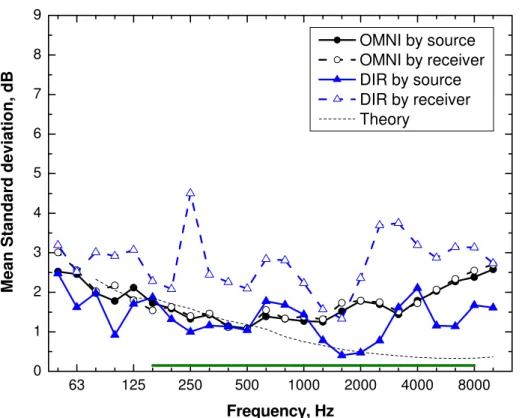
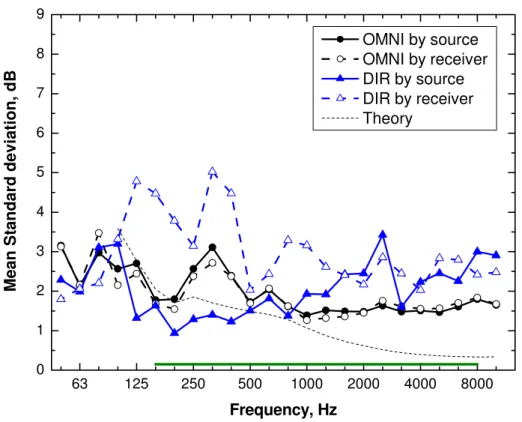
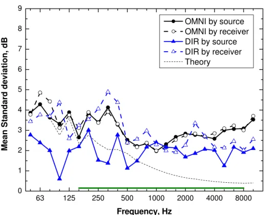
The results of examining the benefits of DIR-IN versus DIR-OUT, compared with the OMNI source, are included in a second set of graphs in Appendix 1 (Figures A1.12 to A1.22). These graphs compare the average spatial standard deviations in the 11 meeting rooms for 3 source conditions along with the theoretical predictions. The 3 source conditions were (a) OMNI source at varied positions throughout the room, (b) DIR source pointing into the two opposite corners of the room, and (c) DIR source pointing out of the two opposite corners of the room. These results were summarised by

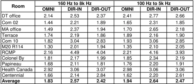
calculating average standard deviations over frequency for each of the three source types/conditions and for each of the 11 rooms. These are given in Table 5.1 below. Averages were calculated over two different frequency ranges: (a) 160 to 8k Hz

corresponding to frequencies important for speech, and (b) 100 to 5k Hz corresponding to

Table 5.1 Average spatial standard deviations of sound lev

standard measurement frequencies in building acoustics.

els (in dB) for the OMNI rent

deviations are consistently smaller for measurements using the tions

e 5.1 and Figures A1.12 to A1.22 indicate that larger spatial variations occur when a directional source is used no matter which orientation is used. There are

OMNI DIR-IN DIR-OUT OMNI DIR-IN DIR-OUT

DT office 2.14 2.53 2.37 2.41 2.77 2.66 Com 02 1.44 2.21 1.89 1.65 2.31 1.85 MA office 1.49 2.37 1.94 1.70 2.65 2.18 Terrace 1.74 2.19 1.86 1.89 2.16 1.90 Com 10 1.82 3.04 2.83 1.93 3.06 2.85 M20 R114 1.30 2.01 1.94 1.35 2.10 2.05 RCMP 2.16 4.49 4.04 2.21 4.16 3.93 Colonel By 1.81 2.17 1.99 1.85 2.34 2.19 Papineau 1.68 2.11 1.81 1.76 2.20 1.91 Health Canada 2.92 3.06 3.07 2.98 3.06 3.06 Centennial 1.66 2.14 2.84 1.62 2.20 2.61 Average 1.83 2.57 2.42 1.94 2.64 2.47 Room 160 Hz to 8k Hz 100 Hz to 5k Hz

source, the DIR-IN source and the DIR-OUT source in each room and over two diffe frequency ranges.

The spatial standard

OMNI source in all rooms. There are only small differences in spatial standard devia between the results for the IN and OUT sources. On average, using the DIR-OUT source leads to slightly smaller spatial standard deviations than when using the DIR-IN source. Calculations over the two different frequency ranges led to similar overall averages.

(22)

differences between the measurements using the two different orientations of the DIR source, but they are quite small and not practically important.

5.2 Required number of source and receiver positions for precise source average room levels

As discussed in section 5.1, for frequencies relevant to speech, the variations of sound levels in rooms are mostly statistical in nature. The average of several measurements at

f positions that can be included. This o ms to r the d ar y

e necessary to obtain quite precise f

s

e to have a different positions can be made more precise by including measurements from a larger number of statistically independent positions.

Although making measurements at a larger number of independent positions is always better, there are practical limits to the number o

section explores the number of combinations of source and receiver positions required t achieve a specified precision. The precision of an average level can be specified in ter of the standard error, SE, of the mean values. (See equation A1.6 in Appendix 1). The SE values were calculated for spatial standard deviations, σ, averaged over frequency to get a single number estimate of the required number of measurements achieve a specified precision in the mean result. These SE values, from standard deviations, were averaged over the speech frequencies from 160 to 8,000 Hz. Since the variations in levels over source position and over receiver position are the same fo OMNI source, the SE of the mean level was determined for the combined variations of both source and receiver positions for this source. The number of measurements require (i.e. number of source and receiver combinations) to achieve SE values of ± 0.5, ±1, ±2, and ±3 dB were calculated. The numbers of measurements to achieve SE values of ± 0.5 dB are given in Table 5.2 for each of the 11 meeting rooms. (The numbers of

measurements to achieve larger SE values are included in Table A1.3 in Appendix 1). Table 5.2 and Table A1.3 show that the number of measurements required for a particul SE value varies considerably with the characteristics of the room and with the required level of precision (i.e. the required SE of the mean value). While achieving a SE of ± 0.5 dB requires between 7 and 35 measurements, a SE of ± 2.0 dB can be achieved with onl one measurement in most rooms. These SE values indicate the expected error of the mean source room level averaged over frequency. The expected errors in each 1/3octave band

could be larger and would vary with frequency.

Because speech intelligibility and audibility vary rapidly with speech level near the thresholds of audibility and intelligibility, it may b

mean source room sound levels. Although Table 5.2 indicates the required number o measurements to achieve SE values as small as ± 0.5 dB, the number of measurement required at independent positions might not be possible in some rooms. For example, Room DT office is a small office with a volume of 56 m3. The 19 independent measurements required to achieve a SE of ± 0.5 dB would be difficult if not impossibl fit into such a small room. In such rooms, space-average values will necessarily little larger SE values.

(23)

OMNI DIR-IN DIR-OUT Room Volume, N for N for N for

m3 SE=±0.5 SE=±0.5 SE=±0.5

DT office 56.00 19 26 23 Com 02 58.01 9 20 15 MA office 65.84 9 23 15 Terrace 107.86 13 20 14 Com 10 206.82 14 37 33 M20 R114 225.67 7 17 16 RCMP 229.50 19 81 66 Colonel By 233.28 14 19 16 Papineau 379.23 12 18 14 Health Canada 512.73 35 38 38 Centennial 518.48 11 19 33 Average 235.77 14.7 28.9 25.7

Table 5.2 Number of measurements required to achieve standard errors (SE) of the mean values (averaged over frequency) of ± 0.5 dB using OMNI, IN, or DIR-OUT sources.

Similar estimates of the required number of measurements to achieve these same average SE values were carried out for the measurements using the DIR source. Because the effects of varied source condition were quite different than the effects of varied receiver position for the DIR source, these estimates were separately determined for the cases with the DIR source pointing into the corners and the DIR source pointing out of the corners. The results are also given in Table 5.2 and indicate that more measurements would have to be made to achieve a particular SE value when using the DIR source than when using the OMNI source. For the average of all rooms shown in the last line of this table, about twice as many measurements would be required when using the DIR-IN source compared to when using the OMNI source. Using the DIR-OUT source would require almost as many measurements as the DIR-IN source. These calculations confirm that using a directional sound source would significantly increase the required number of

measurements to meet a particular level of precision of the source room-average sound levels.

These calculations of the required number of measurements were based on the average standard deviations of source room sound levels over all frequencies important for speech intelligibility (160 to 8k Hz). By ignoring variations with frequency, a simple estimate of the required number of measurements could be made. It is assumed that these frequency-averaged values would relate to average speech levels in the meeting room.

The related variations in SE values versus 1/3 octave band frequency were also

determined for each room. These were calculated for the numbers of measurements required to meet an average SE value for each room as specified in Table 5.2. The resulting SE values versus 1/3 octave band frequency tend to be close to 0.5 dB (see

Figure A1.23). Only at the lower and higher speech frequencies do SE values increase above the average of 0.5 dB. These results support the approach of determining the required number of measurements from the frequency-averaged spatial standard deviations of the source room sound levels. When the number of measurements is

(24)

source or Tables A1.4 or A1.5 for the DIR source), the characteristics for each room are quite similar and hence we would expect similar accuracy of mean values from this procedure.

5.3 Summary of results of source room level measurements

The combined effect of using a number of different source positions should excite the source room to meet the following requirements:

Create a homogeneous average distribution of sound levels throughout the room so that the mean level can be precisely determined from a reasonable number of measurement positions.

Create a homogeneous distribution of sound levels incident on all boundaries of the room and arriving from all directions so that sound transmission through all boundaries can be considered relative to the same source room level measurements.

The measurements presented in this section and in Appendix 1 address the first

requirement. The second requirement is considered by the results presented in following sections of the report.

The results here present considerable evidence to support the need to use an directional sound source for the proposed speech security assessments. Using an omni-directional source leads to a more homogeneous distribution of sound levels throughout the meeting room. Because the variation of levels throughout the room is less with an omni-directional source, we can determine the mean source room sound levels more precisely. Alternatively we can say that fewer measurement positions would be required to achieve some level of precision than would be required using a directional source. We used positions of the directional source in the opposite corners of the source room. This was intended to provide conditions where the directional source might be more comparable with the omni-directional source. However, even for these directional source positions, spatial variations were greater with the directional source. Although not tried in these tests, using a number of directional source positions throughout the meeting room would be expected to lead to greater problems because at some frequencies microphone positions could be in the direct field of the loudspeaker source. The other disadvantage of using directional sources located in the opposite corners of the room is that source room measurements must be repeated for each different boundary of the room making the total measurement time much longer.

(25)

6. Sound Transmission Measurements

Sound transmission measurements were made from the 11 meeting rooms to adjacent spaces. The details of the measurement positions varied from room to room depending on the room size and the complexity of adjacent spaces. As described in section 3.2, sound level attenuations were measured from various room-average measurements in the source room (the meeting room) to both spot positions, 0.25 m from the outside boundaries of the room, and to space-average measurements in the receiving space.

From the sound transmission measurements, four different indicators of speech security were calculated for both spot measurements and receiving space-average measurements. These were: (a) an A-weighted transmitted speech level, (b) an A-weighted speech – noise level difference, (c) SNRSII22 values, and (d) SNRUNI32 values. In all calculations a

space-average speech level in the meeting room of 69 dBA was used corresponding to the 98th percentile speech level measured in meeting rooms [1]. An ambient noise level of 36 dBA with a – 5 dB/octave spectrum shape, corresponding to a 2nd percentile day-time noise level in spaces near meeting rooms [1], was also used in calculating the signal-to-noise ratio measures. The A-weighted transmitted speech levels and the A-weighted speech – noise level differences provide essentially the same information offset by 36 dBA. However, both are included for the convenience of the reader. For each of these 4 measures, values were calculated for 3 different methods of obtaining source room-average levels. These were: using the omni-directional source (OMNI), using the directional source pointing into the two opposite corners (DIR-IN) and using the directional source pointing out of the two opposite corners (DIR-OUT).

All values of the 4 speech security indicators are given in Appendix 2 with floor plan sketches for the 11 meeting rooms. In this section only the values of one measure

(SNRUNI32) are presented for 5 rooms, to illustrate the types of effects that can be found.

6.1 Results for a small room with no door in test wall

The simplest case is a small meeting room and tests of sound propagation through a wall without any doors. Figure 6.1 for the DT office illustrates the results of SNRUNI32 values

plotted versus spot measurement position along the test wall in the adjacent room. For this case the SNRUNI32 values, obtained using the different types of source, are quite

similar and the values do not vary greatly with spot measurement position. The receiving space-average results are approximately an average of the spot measurement position results.

There is a small trend for SNRUNI32 values to decrease from left to right on this graph.

This was probably due to the wall construction changing across this wall. Near the positions to the left of the graph, the wall construction was gypsum board on steel studs, but to the right of this graph the wall changed to a more massive construction. Although spot position results were almost identical for the OMNI source and for the DIR-IN source, the DIR-OUT results are approximately 1 dB lower in value. The irregularity in the DIR-OUT results at position 7 was thought to be due to a minor leak via a ceiling duct system. For the receiving space-average results the OMNI source result is closer to the DIR-OUT results than the DIR-IN result. In spite of some small irregularities, all of the types of measurements in Figure 6.1 provide roughly similar information.

(26)

Avg 1 2 3 4 5 6 7 -10 -8 -6 -4 -2 0 2 4 OMNI DIR-IN DIR-OUT SN R UNI 3 2 , dB Position 1 2 3 K1 K2 4 5 6 7 4.79 m 3.95 m Height 2.96 m DT Office Source room Avg Figure 6.1 DT office (Room volume 56.0 m3)

(27)

6.2 Medium sized room with two doors in the test wall

The results in Figure 6.2 are for M20 Room 114, a medium sized meeting room with a room volume of 225.7 m3. In this case the results are for a test wall that included two doors that were obvious sound leaks. The location of the doors is quite obvious in the plot of SNRUNI32 values (positions 2 and 11), and the measurements correctly reflect the

significant sound leaks.

This room has quite diffuse acoustical characteristics with relatively low spatial standard deviations of the source room levels as illustrated in Figure A1.16. This probably

contributes to the close similarity of the SNRUNI32 values calculated using the OMNI,

DIR-IN, and DIR-OUT sources. Although the receiving space-average results may approximate an average of the measured spot position results, they do not provide any information concerning the serious leaks at the two doors.

6.3 Small room tested on two different walls

Figure 6.3 illustrates results for the MA Office that includes propagation through a wall without doors into the room to the right of the floor plan, and also through another wall with a door to the bottom of the floor plan. This results in two quite different sets of results shown on the upper part of this figure.

The left side of the plot of SNRUNI32 values shows the results for propagation through the

wall without doors to positions 1, 2, 3, and 4 in the adjacent room on the right of the floor plan. There are differences between the results for the different source types and the OMNI source results indicate higher SNRUNI32 values by up to 1 or 2 dB. That is, the

DIR-IN and DIR-OUT results underestimate the lack of speech security by a small amount depending on the position. Also the corresponding receiving space-average results (to the left of the graph) underestimate the lack of speech security by 3 to 4 dB compared with the spot measurements. This may be due to the difficulty of getting good average results in this receiving space, which included a partial height office screen between the two desks that filled a large part of the room.

The results for the other wall, that included a door, are shown to the right of the same graph. The SNRUNI32 values decrease rapidly when moving away from the position of the

door (Position #5). The door was an obvious sound leak that included a vent that had been inadequately covered. Again for this wall the receiving space-average results do not reflect the possible lack of speech security that exists at positions close to the door.

(28)

Avg 1 2 3 4 5 6 7 8 9 10 11 12 6 8 10 12 14 16 18 20 SNR UNI3 2 , dB Position 1 2 3 4 5 6 7 8 9 10 11 12 K1 K2 Avg _Hall 11.36 m 6.61 m Ceiling height 3.00 m Figure 6.2 M20 Room 114

(29)

Avg 1 1 2 3 4 Avg 2 5 6 7 8 -10 -8 -6 -4 -2 0 2 4 6 8 10 OMNI DIR-IN DIR-OUT SN R UN I3 2 , d B Position K1 K2 K3 1 2 3 4 5 6 7 8 5.13 m 4.25 m Height = 3.02 m Avg 1 Avg 2 Figure 6.3 MA Office (Room volume 65.8 m3)

(30)

6.4 Larger room with double door and vestibule

Figure 6.4 shows results for the Centennial room which is a larger space with a room volume of 518.5 m3. The spatial standard deviations of the source room levels in this room (shown in Figure A1.12) are larger than in other rooms such as M20 R114. Thus the sound levels incident on the test wall, and in particular on the doors in the test wall, could vary considerably between the results for the different source types.

This effect is indicated in the results shown in the graph of Figure 6.4, where the

SNRUNI32 values systematically vary among the three source types used. In addition, the

differences among the source types systematically vary with position along the test wall and are largest at the position of the main door. At this location (position #4), the

SNRUNI32 values from the OMNI source results are about 3 dB higher than the SNRUNI32

values from the other sources indicating apparently lower speech security.

For this room the degree of speech security, although never high, varies considerably along the test wall and the doors are again an obvious weak spot. This is in spite of the use of a double door system. The receiving space-average results do not provide useful information about the large variation of the level of speech security with position along this wall. The results obtained using the DIR source significantly overestimate the degree of speech security.

6.5 More complex larger room

Figure 6.5 shows results for the Health Canada EOC Room. This was a larger volume room (516.7 m3), with large spatial variations in the source room measurements shown in Figure A1.20. The room was fitted with a ring of fixed desks and included a

significant amount of absorbing material. One would expect these features to lead to different incident sound levels from the various source types on the test walls in this room.

For the measurements at positions 1-8, the OMNI source results lead to higher SNRUNI32

values and indicate lower speech security than for the DIR sources by up to about 4 dB. The DIR-IN source results lead to higher SNRUNI32 values than when using the DIR-OUT

source.

For the position 9 to 12 spot measurement results, the DIR-OUT source results lead to higher SNRUNI32 values. This is presumably due to the directionality of this source even

though it was located in the corners across the room from the test wall.

Although two sets of receiving space-average results are shown on Figure 6.5, it was difficult to make meaningful space-average measurements in the spaces adjacent to this room. The area near positions 1 to 8 at the bottom of the plan was a large open office area. The space-average measurements were made in the small corridor area near to one of the doors to the meeting room. They seem to be somewhat representative of levels near the door but not of those conditions further along the wall. Similarly, the measurements at positions 9 to 12 were in a small open secretarial area that was again quite ill-defined. The conditions near this room are a good example of conditions where space-average receiving measurements are not particularly useful and illustrate the value of the spot measurement approach.

(31)

Avg 1 2 3 4 5 6 7 8 -14 -12 -10 -8 -6 -4 -2 0 OMNI DIR-IN DIR-OUT SNR UN I3 2 , d B Position 1 2 3 K1 K2 4 5 6 7 9.69 m 12.77 m Height 4.19 m Translation booth Outside 8 Centennial Room Translation booth Hall 9 Lounge 10 Avg

Figure 6.4 Centennial Room (Room volume 518.5 m3)

(32)

Avg 1 1 2 3 4 5 6 7 8 Avg 2 9 10 11 12 -10 -8 -6 -4 -2 0 2 4 OMNI DIR-IN DIR-OUT SN R UN I3 2 , d B Position K1 K2 K3 K4 4 m 12.4 m 9.77 m Height 3.0 m (3.38 m centre) Secretary station Open office cubicles in closed room Open-office area 9 10 11 12 Hall Avg 2 Hall Hall 1 2 3 4 5 6 7 8 Avg 1

Figure 6.5 Health Canada EOC Room (Room volume 518.7 m3)

(33)

6.6 Summary of room-average to spot-receiver sound transmission measurements In smaller rooms the directional source results can be similar to the omni-directional source results. However, in larger rooms and especially those cases where there are large spatial variations in the source room, the directional source results can significantly overestimate the degree of speech security. Differences in SNRUNI32 values of 3 dB or

more can occur and these could correspond to large differences in the numbers of people being able to overhear speech near these rooms. The largest differences between the results for the different source types occur for rooms that are greater than about 200 m3 in volume and have large amounts of sound absorbing material in them, leading to larger spatial variations in the source room.

The use of a directional source can lead to consistently lower values of signal-to-noise ratio speech security rating measures and in some cases the effect of source type can be much larger for positions near weak spots such as doors.

The new results clearly demonstrate the advantage of spot measurements over receiving space-average results. Where there are weak spots and the spot measurement results vary significantly with position along a test wall, the receiving space-average results cannot indicate this range of results or help to locate leaks and weak spots in the sound

insulation. The average values may approximate the average of the various spot

measurement position results, but often they will not depending on the relative locations of the two types of measurements. In many cases it is not possible to define a suitable area to represent the average receiving space.

6.7 Comparisons of simple SET method with room-average to spot-receiver results Various people have proposed simple speech security tests intended to evaluate sound transmission through a particular element of a room boundary such as a door. In these simple tests the source is pointed at the door and sound levels are measured either side of the door. Figure 6.6 illustrates the experimental setup for such a test referred to as the SET or Single Element Test method. The sound source is located 2 m from the test object, which is a door in this figure. The microphones are located 1 m either side of the door. Sound attenuations are calculated between the levels measured at the two

microphones. Often in the past, only A-weighted level differences have been used to characterize the wall element under test.

In the current work similar measurements were made in most of the rooms tested and with the DIR source and the microphones located as illustrated in Figure 6.6. From the attenuations between the levels measured at the two microphones, and using the same speech and noise levels as in the previous results in this chapter, values of the three signal-to-noise ratio measures were calculated, i.e. (a) an A-weighted speech – noise level difference, (b) SNRSII22 values, and (c) SNRUNI32 values. These results were then

compared with the previously discussed results in which these same three signal-to-noise ratio measures were calculated from room-average values to spot-receiver measurements using an OMNI source. The differences between the two methods are illustrated in Figures 6.7, 6.8 and 6.9.

(34)

1 m 1 m 1 m

Loudspeaker Microphone

Microphone

Figure 6.6 Experimental setup showing location of the DIR sound source and the measurement microphones for the simple SET type of measurements.

Figure 6.7 plots the differences in SNRSII22 values obtained from the SET method less

those obtained from the complete room-average to spot-receiver position method. Figure 6.8 and Figure 6.9 illustrate similar differences for SNRUNI32 and A-weighted speech –

noise level differences (ΔdBA). In these graphs, positive differences indicate that for the SET method more sound energy was transmitted through the test element. Negative differences indicate that the OMNI source complete method transmitted more sound energy through the test element. There are large positive and negative differences that mostly vary with the particular conditions in each room. The results in Figure 6.8 for

SNRUNI32 values are discussed for continuity with the previous parts of this chapter, but

the results in the other two plots show almost identical trends.

The largest positive differences occurred in the RCMP room. They are thought to be due to the room-average to spot-measurement approach including some additional attenuation from the locations of the room-average measurements to the location of the door. As the floor plan of this room shows (Figure A2.10), the entrance door is located behind a screening wall that separates the main part of the room from the entranceway. This room was unusual too in that the walls were all very highly sound absorptive. Thus, it is quite likely that sound propagating from the room-average positions to the door would be attenuated significantly. This does explain the differences between the two test methods, but does not indicate a problem with the room-average to spot-receiver measurement procedure. The method is intended to assess the speech security for sound sources representing people talking in the meeting room and the OMNI test source was quite appropriately located at positions where people using this room could be located. Most of the negative differences in Figure 6.8 are for tests associated with Committee Room 10 (Com10) and Committee Room 02 (Com02). These rooms had a suspended T-bar type ceiling that did not seem to extend fully to the floor deck above. Although it could not be verified, it sounded like a significant amount of sound energy somehow passed through the ceiling void. Since the DIR source used in the SET type

measurements was pointed directly at the test element and located about 1 m above the floor level, less sound energy would be directed up towards the ceiling. Of course, the

(35)

energy from it towards the ceiling, which could more easily be transmitted via the ceiling void into the next space. This is thought to explain the majority of the negative

differences. Com10-9 #4 Com02 #1 Com02 #3 Com10-9 #3 Centennial #9 Com02 #1 Com02-Hall #3 Health-Open #2 Papineau #4 Com10-P #2 Centennial #10 Colonel By #5 Papineau #1 Health-Office #2 M20R114 #2 MA-Sec #1 Centennial #4 M20R114 #11 RCMP #4 RCMP #3 RCMP #1 -8 -6 -4 -2 0 2 4 6 8 10 12 SNR_SII22 differences, dB

Figure 6.7 Differences between the OMNI source room-average to spot-receiver results and the simple SET approach for SNRSII22 values.

Com10-9 #4 Com02 #1 Com02 #3 Com10-9 #3 Centennial #9 Com02 #1 Com02-Hall #3 Health-Open #2 Papineau #4 Com10-P #2 Centennial #10 Colonel By #5 Papineau #1 Health-Office #2 M20R114 #2 MA-Sec #1 Centennial #4 M20R114 #11 RCMP #4 RCMP #3 RCMP #1 -8 -6 -4 -2 0 2 4 6 8 10 12 SNR_UNI32 differences, dB

Figure 6.8 Differences between the OMNI source room-average to spot-receiver results and the simple SET approach for SNRUNI32 values.

There are other problems with the SET approach that will lead to less reliable results and that may explain some of the other differences between the two methods. Because the DIR source is deliberately located close to at least two room boundaries (wall and floor)

(36)

and the microphone assessing the source room level is even closer to these reflecting surfaces, there can be significant interference effects that could greatly change measured source room levels at particular frequencies. Small differences in the locations of the DIR sound source or the source room microphone could greatly affect the measured signal-to-noise ratio values. The same type of door construction located in different rooms could lead to quite different results. Configurations such as that illustrated in Figure 6.6, where the door to be tested is close to the corner of the room, could further complicate

measurements by adding strong reflections from a third nearby surface.

The generally large differences in these plots clearly indicate that the Single Element Test is not a reliable test method.

Com10-9 #4 Com02 #1 Com02 #3 Com10-9 #3 Centennial #9 Com02 #1 Com02-Hall #3 Health-Open #2 Papineau #4 Com10-P #2 Centennial #10 Colonel By #5 Papineau #1 Health-Office #2 M20R114 #2 MA-Sec #1 Centennial #4 M20R114 #11 RCMP #4 RCMP #3 RCMP #1 -10 -8 -6 -4 -2 0 2 4 6 8 10 ΔdBA differences, dB

Figure 6.9 Differences between the OMNI source room-average to spot-receiver results and the simple SET approach for ΔdBA values.