Asymmetric inlet flow in axial turbomachines

r-7 Hw- -4, 7 0Y 1111 , Q V P It ki, U-1 x1Q1,10 *i Tw T 'N Nil Mo. V, A-M 2 ... .... . 4 n-,

-Awliq cab -way Ell

... ... .. .. -u m Ila IM 4 k ... .. now mails mh vvm : .: go got INMAN tk Una CV ONE 3 TWO Two AWK-s" kv-it: 14 Wow '4 f"Now 460 , MO= Wv 4, M . . . ............. ... .. .. L p 7 . .......

by

BARRY S. SEIDEL

Under the Sponsorship of: General Electric Company Westinghouse Electric Corporation

Allison Division of General Motors Corporation

Gas Turbine Laboratory Report Number 51

May 1959

ACKNOWLEDGMENTS

ABSTRACT

1. INTRODUCTION

2. ANALYSIS

2.1 Description of the Flow Field and Governing Equations 2.2 Boundary Conditions at the Blade Row

2.3 Translation of Boundary Conditions to Relations in 2.4 Determination of the Blade Forces

2.4.1 Blade Force Caused by Velocity Perturbation

Normal to the Mean Relative Velocity Vector (Sears Force) 2.4.2 Blade Force Caused by Velocity Perturbation in

the Direction of the Mean Relative Vector (Isaacs Force)

3. EXPERIMENTAL INVESTIGATION

4. COMPARISON OF ThEORY AND EXPRIMENT

4.1 Comparison of Blade Force Predictions

4.2 Comparison of

6'1

4.3 Effects of Flow Rate and Solidity 5. CONCLUSION

APPENDIX I

APPENDIX II

APPENDIK I

APPENDIK IV

A Boundary Relationship Between Two Cauchy-Riemann

Variables

u, V, p -/.,@) Equivalence; Translation of Boundary Conditions to Relations in //4 (

Tabulation of the

Description of Computation (Programming) A4.1 Main Body of the Present Theory

A4.2 Sears Force

A4.3 Isaacs Force

A4.4 Rannie-Marble Theory

3

3

6

8

11

12

15

18

22

23

23

25

27

28

36

38

38

40

42

46

LIST OF SYMBOLS 50

The author expresses his gratitude to the staff of the Gas Turbine Laboratory. _{Professor E. S. Taylor, Director, continually} brought the major issues into focus. Professor Alan H. Stenning served

as thesis supervisor and guided the early part of the work until his de-parture to the Nuclear Engineering Department. Professor Yasutoshi Senoo

then became thesis supervisor. Professors James W. Daily and Alve J. Erickson served on the thesis committee. Their continual guidance and

suggestions are indeed appreciated. Also, helpful discussions on the problem were held with Dr. F. Ehrich (General Electric Co.) and with

Professors H. Emmons and C. C. Lin.

For providing experimental information on this problem, the

author thanks Lieut. (U.S.N.) Frank Carter, Joseph Jennings and Captain (U.S.M.C.) Marvin S. Shinbaum, who also lent valuable assistance in other phases of the report. Messrs. Dalton Baugh, Basil Kean and Paul

Wassmouth aided in the use df the laboratory equipment and provided

pre-cision mechanisme and probes. In computation and graph preparation the

author was aided by Messrs. James Brown, Charles Haspel, and James Hurley.

This work was done in part at the M. I. T. Computation Center,

Cambridge, Massachusetts. The author is grateful for the use of the IBM

704 Electronic Data Processing Machine.

Typing was ably performed by Natalie Appleton.

Finally the author is grateful to his family and especially

A modified actuator disc analysis is made which, through an

im-proved prediction of the blade forces, attempts to give closer correspond-ence with experiment than the previous theory. The fluid is assumed in-viscid and incompressib2le. Perturbations to the two-dimensional flow through an isolated blade row are considered. The steady flow equations of motion and continuity are linearized.

According to experiments conducted on an isolated compressor rotor, the present theory offers an improvement, compared to previous theory, in the prediction of distortion attenuation, effects of flow rate, and effects of varying chord/spacing ratio.

1. INTRODUCTION

The problem of gsymmetric inlet flow, or circumferential distor-tion, in axial turbomachines is quite simply stated. The velocity of the flow far upstream of any blade row may in general vary with the radius r, the angle Q, and even with time t. Because in the 'normal' (classical po-tential flow through cascades) situation the velocity far upstream is r-@-t independent, the flow in problems in which one of these variables assumes a non-trivial role is spoken of as 'distorted'. In the asymmetric inlet flow problem here considered, 9-dependency alone is studied. The problem

is thus: given the properties of the inlet flow (as a function of 9) and the characteristics of the blade row (s), to determine the properties of

the fluid everywhere in space.

In the actual turbomachine these distortions may occur when the

engine is operated at an off-design condition, when the aircraft is flown at high angles of attack, or when the flow is turned, or diffused too rapidly within the intake duct.

In the solution to the problem one would also like to know the

perturbations in blade force from their mean value (and how to minimize them), the attenuation of the distortion through the blade row (and how to maximize this quantity) and the overall effects on compressor perfor-mance.

Linearized actuator disc solutions to this problem have been

the relative angle of the flow leaving thp rotor is constant and that there are no losses in the flow relative to the rotor. Rannie and Marble have gen-eralized to allow both of these quantities to be functions of the relative inlet angle to the blade row. Ehrich's theory is for an isolated cascade;

Rannie and Marble also treat finitely spaced:>blade rows. Although these

tm: theories utilize completely different mathematical techniquep they do give the same result for the conditions of isolated cascade, no losses,

con-stant relative leaving angle. Indeed they must give the same result, by the

uniqueness principle. Since the conditions mentioned are used throughout

this report in computing the predictions of the previous theory, in this sense we have only to acknowledge the existence of a single previous theory.

The mathematical technique of Rannie-Marble has been used throughout and hence the previous theory is labelled "Rannie-Marble". It is understood that Ehrich gives the same prediction.

2. ANALYSIS

2.1 Description of the Flow Field and Governing Equations

Let x, y be -rectangular

coordinates

with the axis of y parallel

to the plane of the cascade, Figure 1. The average velocity components and

pressure of the undisturbed uniform flow are U, V and P, constant upstream

and downstream respectively. The circumnferentially distorted flow is

repre-sented by superposing a disturbance flow on the uniform flow. The

distur-bace velocity compozints and the dist,4rbance pressure are u, v, p, all

with space average values zero. The disturbance is

assumed to be periodic

in y direction. The disturbance flow treated here is due to non-uniform

upstream flow and its interaction with the cascade as a whole; local

dis-turbances

due

to individual blades

are

not considered.

Thus, as will

sub-sequently be seen, one may consider this to be a "modified" actuator disc

analysis. The fluid is assumed inviscid and incompressible; the flow

field is considered two-dimensional.

Under thepe circumstances, the equations of motion and continuity

in linearized form are

U-

=--U

VM

-Zr

2

ax

C)

In the place of these famil4ar equations we choose to use the following three, completely equivalent equations:

U

-t

V

{

Y e

+-

V

?'r 0

=4

S

(U-VMw)

= ~

(

)

5

Equation 4 is simply the condition that the perturbation in total pressure is constant along the mean streamlines. Equations (5) and (6)

show that the combination Uv - Vu (proportional to flow angle perturbation) and the static pressure divided by density satisfy the Cauchy-Riemann con-ditions. It is convenient to introduce the definitions/

H=

/

lf

t U

tf

Vz-

7

U

-

Vit

8

U

9

the following relations then hol4

00, V

x)

10

The establishment of equations (11) and (12) constitute a major step toward the solution, for now, all of the power of potential theory can be brought to bear, at least on G and 6 . We are able to use

po-tential theory, not on u and v (since the flow is not irrotational), but on two other functions

(

,

9

)

A particularly useful example of the functional relationship be-tween z and (9 is developed in Appendix I . Consistent with our

as-sumption of an isolated blade row lying along the y axis, it is there shown that for ((o, y) given, 6? (0, y) can then be found from

6

0 t

(

t( / ?)cY74-

s(0

.)

_13

similarly

e

o-,

y)=6

N-7oy

₄

₎

The borrespondence 'between this appendix and the main body of the text

is as follows: Text Appendix u x' v

x

x

Since 9 and

P

satisfy the Cauchy-Riemann conditions, they may

be found for all values of x and y if the boundary values 9 (o, y) or

(o, y) along the blade row are given.

Finally, in order to relate

0

or

69

to u and

v,

H(x, y)

=

H(o,

y

-

Y

x) must be known.

U

2.2 Boundary Conditions at the Blade Row

(a) Axial Velocity Match Condition

Since we

are neglecting any change in density through the blade

row, and the annul14s area is constant, the axial velocity entering the blade

row must equal the axial velocity leaving the blade row.

Letting station

1 represent the line x

O-(just upstream of the cascade) and station 2

the line x

=

O+(just

downstream of the cascade) we have then that

Obviously, the average axial velocities are the same upstream and

down-stream and so we have simply that

JL

(0-)

(0 y)

or

jL,

4L

15

(b) Quasi-Steady Bernoulli Equation; Relative to the Rotor

We define a loss coefficient CD(0l) such $hat the Bernoulli

equa-tion for the mean flow may be written

L U

sf u'

(v -n

r)

-7

=

/0, Z

s ub

v.-a r '_7 + zf 'o'

Then the condition for the perturbed flow, obtained by taking the differential

of

_{the previous equation,}

Also, since

47d

/4

Alternatively.

a r-

_{U -}

Now we may rewrite (16),

(c) Prescription of the Blade Force

COGS1CD

S/3

157

)-

r-it

C;

The force parallel to the blade row corresponding to the mean

flow

is

-

=f Su (V-

V2)

17

when the inlet flow has a distortion, this force is composed of a mean

value -

4"

A

obtained by taking the differential of the previous equation is

-l

4~I>

(c~S

7 -.12 r&

Cos

_,yl

16a

U

hr

-

Y'

)

t'u

,

v-

v

)

2.3

Translation of Boundary Condition to Relations in

We -now require these matching conditions in terms of the

func-tions

6

Equation (15) becomes (Appendix II)

~

19

The

5

are known constants.

Equation (16a) becomes

gz -e

(//z

-6 0'2

-

e

20

Again, the

S are known constants.

Equation

~

0~

2

@

7(

2

,-7S?16

Ma)(/

-

0-

cq

7L6,1

21

or letting

z-

C2S

(7

6Qg

-lg

Z)

<0

2 cs"9,ba:15le~)e6,

(21) becomes

F

22

We now choose to eliminate the H

in equation (20). From (19)

letting

S

S=p/d

el3

p

(23) becomes

23a

Substituting this value of H2 into (20), we obtain

=

6f

4/1V(l)-s9

_74L

(Z

letting

(24) becomes

el4s. F1

)t

s4-

,2

7M6-

e2-

Ozs

,

25

217eZ7e

24

t (9-6(!5 ).

z

6|*& ta6|)*

IL4

?/, Y = 5 ' ell

6 /-sPA&)

-622

,(P.

tfl

-

(45

7sF1

)62

,(P

7s

)

- el5-

P

)

e

-S

=e

=5 01V

-e2

(25) becomes

(22 7 r to give

(22) may be rearranged to give ₆

e- ) -

5169

letting

(27) becomes

szo (F2 ~

=

For reference we recall (26)

5'-

-9S e

-

operate on equations (28) and (26), using thej of complementary functions to obtain

-O612

-g e ;' - /// )

63 10

(

7"

26

previously developed

29

30

The four linear equations (28), (26), (29), (30) are sufficient to

de-termine

9,

_OZ

_{in terms of the fuxxtions Hl, H*42}

H2 may now be determined from equation (23a), completing the solution.

In this entire section the blade force has been treated as a

known quantity.

The manner in which blade force is actually obtained is

discussed in the

subsequent section.

26

27

28

We now

notion

5 fo

= /-?/0

As we have seen, as the blade passes through the distortion, it

incurs _{a perturbation in force directly related to the mean flow and to} the perturbations in the mean flow. At any instant (or y location) a given airfoil is subdect to a perturbation in velocity. The velocity perturba-tions which affect the airfoil lift are up, uo_, vo and vo_. Specifically

as has been discussed in Reference 18, the lift is affected by . = (uo + uO_)/2 and by v = (vo. + vo_)/2. Thus the total velocity perturbation is given by

u +. _{v, as shown by the dashed line in Figure 2. The li"'t in uniform flow,}

as is well known, is determined by the mean relative velocity vector w0.

It is both natural and fruitful to resolve the total velocity perturbation along and normal to wo. As is shown in Figure 2, we have

called ur, the component along w0 and vr, the component normal to wo. In

the Figure as drawn, vr is inducing a negative perturbation in force on the blade, hence the minus sign.

As is obvious by inspection, by simple resolution of vectors,

LL= CO5(''4 -

?

Conversely

Here u and v may be found, as a first approximation, from the previous

theory (Rannie-Marble).

Thus a given airfoil in cascade is subject to both a time vary-ing yr _{and a time varying ur, both of course periodic of period equal to}

the period of the distortion. _{The determination of the time varying lift} of an airfoil in cascade under the influence of either of these velocity

*

perturbations has not been solved.- Therefore, the author suggests the somewhat simpler model of a single uncambered flat plate airfoil subject to time varying ur and vr; the influence of other airfoils would then be treated by the lattice coefficient (Ref. 28) notion or its equivalent.

Each velocity component would be treated separately and the resultant blade forces added algebraically.

A solution to tbe fluctuating ur problem has been obtained by

Isaacs, Ref. 17. A solution to the fluctuating vr problem has been

ob-tained by Sears, Ref. 10. Both solutions are subsequently described.

2.4.1 Blade Force Caused by Velocity Perturbations Normal to the Mean Relative Velocity Vector (Sears Force)

The calculation of the nonsteady aerodynamic lift induced at a thin airfoil by a relative upwash, sucfr as is shown in Figure 3, can be obtained from the results of a paper by Sears, Ref. 10. In this theory, both the impulsive pressure (virtual mass) and the influence of the shed vorticity are accounted for in computing the lift. Sears has shown that

if a thin airfoil experienceg a nonsteady upwash of the form

A solu~ion to the closely related problem of an oscillating cascade is

the time dependent lift is given by

where is the reduced frequency and

S

shown in Figure 4. In this figure note that the magnitude of lift is repre-sented by the modulus of the vector from the origin to the frequency in

question. The phase, with respect to _{the zero frequency lift,} is given by

the angle between this vector and the positive real axis. Note that lim L = 0.

k-> 00

For a distortion of period 21, the appropriate trigonometric form for the primary wave is clearly

(Z

distortion of primary wave length

A

0 2-7r

I

A-a2.t

Thus, in general, the fundamental circular frequency is

Since the lift is determined by the- relative velocity, we may find the lift _{whether the airfoil is sationary and the wave is moving, or}

vice versa. _{In our case, the distortion is, of course, fixed -in space} (stationary) and the airfoil is moving. There is, therefore, a simple

re-lation _{between the variables of time t and distance}

A

The time reqiired for a blade to pass through a complete cycle

is

Now we can represent a periodic gust of arbitrary shape as

-7r

A

n~ &Ck L

and expect to find the lift as

The tangential blade force deviation may now be found from

A

C05

Pmean is defined by the relation

=

.

2

Vz

Therefore

Now

.r~

that we have as a function of time, it is clear that we

may find from the relation

_or

_t

_f

The relation between y, t and _{can best be demonstrated by referring}

to Figure 5.

The wave phenomenon under discussion occurs along the r axis

as showno r is in the /Erection of wo . The time required for the blade to travel from peak to peak along the y axis is

tc =

A r C /-a

-~',

XCC

If the, observer now moves from r = 0 to the point r i with the wave velocity wo, anoadditional time of r , /wO will be required before the

ex-pected peak reaches the observer. Thus in general

and since this is true for arbitrary t, y, we have

rl ~ _(2. / t

2.4.2 Blade Force Caused by Velocity Perturbation in the Direction of the Mean Relative Velocity Vector (Isaacs Force)

As previously discussed, the blade is subject to time varying ur.

The time varying lift _{for such a blade has been given in a paper}

"Air-foil Theory for Flows _{of Variable Velocity", by Rufus Isaacs, Ref. 17.}

This problem and the Sears problem previously discussed are not trivial

problems to solve ch1;Lefly for one reason: in each solution, the Kutta

condition is maintained, airfoil circulation is continuously changing

(circulation is continuously shed) and the effects of the shed circulation

must be taken into account in determining the lift.

The problem is easily represented with the aid of the diagram in

Fig. 6-1. As previously, _{wo is the mean relative velocity vector; a}

si-nusoidal perturbo.tion

6:Tof

Thus the ratio of the instantaneous lift L to the lift L0 is

a function of k and t. _{Graphs of L/LQ versus time t with 6 and k} as independent variables are given in figure 6. These graphs have been computed using the formulae given by Isaacs. These formulae are next described.

For the case in which

Z ro e ~ 7

where

f 3{ zcosu) &t

t(,I

~

+

e-(4,1cos1W

t

7

'W

sin

₄

;

t

t

)]

o,(

,,

F~~

(ne)+g'2,n)

F6J(

)

+/ n/tSt~z-i Tn

F and G are the real and imaginary parts respectively of the Theodorsen function shown in Figure

7.

What we want to have is

AY/

~

7f /M

n

f&L~(zbc S

_i

.5-

_{4C0, Int}

_-+

7'

)7

Fourier generalizing in the usual manner, we find that if the disturbance can be represented as

-=i,

4t=-Z,427r7Yt23

Ss,4

Z7r

/

=/

VTV,-,

4

_{t=-in1-kf 5}

_[

_TL,,,M

_{(n 0)-,, , (4 0+}

G

-

(>/)

zo (

$

_sWet

then the perturbation in force is given by

7/ 74 j Z r / ( t7cosn? 4-L427960 d

Zmr2c5M?,ff

And again, ~

.

Fortunately, the series for 1. converges very

rapidly (because of the rapid convergence of the Bessel functions) both

in n and in m. For example taking m = 2 and n = 5 seems to insure that L/Lo calculated on this basis will not differ from the value implied by the infinite series by more than 2%. ,

As has been discussed, the Sears force and the Isaacs force are finally added algebraically, giving a continuous function of y:

-bu

rzbu

-S

A is the lattice coefficient, the determina~ion of which is discussed in Appendix V. Also discussed in this appendix is the de-termination of the mean incidence im, required in the Isaacs force

com-putation.

Fig. 8 is the rotor

equipment

The experiments were conducted on an isolated compressor rotor. a schematic diagram of the machine; Fig. 9 is a photograph of with 2b/s = .525. Also shown here is the pressure measuring

to be described subsequently.

The essential dimensioni of the compressior are:

Hub-tip ratio 0.75

Tip radius 11.63 inches

Blade chord 1.51 inches (no taper)

Linear twist, root

to tip

_9.7*

No. of blades

44,

at 2b/s

=

1.05

Blade section

Mean radius stagger, measured from the

axial direction Tip clearance 22, at 2b/s =

0.525

NACA 65-(12)10

approx. .035 inches

The constant area annulus extended 29.8 inches upstream and 36.5 inches downstream of the rotor. Radial air flow entrance was through screens. In all tests, the rotor was operated at 1000 rpm. U was of,the order of 50 ft/sec; wo was of the order of 100 ft/sec. A tabulation of Rernolds numbers based on blade chord together with other significant parameters is given in Table I.

TABLE I

2b/s = 1.05

2b/s

U/11r im Re2b U/rt r im Re2b

.562

9.30' 40,500

.514

8.800 36,500

.46o

.391

Two flow rates were studied at each of two solidities. The lower flow rate was, in each case, just above the point of inception of propagat-ing stall. Before any distortion -producing screens were inserted, it was determined that the flow in this case, to the accuracy of the measuring struments, was axisymmetric. Relative position of screen and measuring

in-struments was obtained by rotating the screen, in stepwise faghion, using

the reel and cord arrangement 'shown in Fig. 10. The fact that three screens are shown in this figure is discussed subsequently. The relative location of screen, probes, and rotor is shown in Fig. 11.

As has been mentioned, the distortions were produced by screens, the choice of which is to be described. A photograph of these screens and

their frame holder is shown in Fig. 12. Early in the investigation it was found that one had to make a rather careful choice in the screen or screens to be used. Screens of too high solidity diverted the flow around them so that the requirements of the theory (flow uniform in direction at upstream

infinity) could not be met. Any screen, of course, does this to a certain

extent. However, the screens ultimately chogen produced uniformly axial flow generally to within 50*. The second problem concerned the generation

completely in References 21 and 24 was solved, at least to a large extent,

by reducing the effective solidity toward the edge of the screen. Finally,

the screen had to produce a measurable perturbation that could be considered

within the bounds of a linearized analysis. A trial and error process

re-sulted

in the following description, applicable to each of the three

seg-ments shown in Fig. 12.

a) 45* (circumferential extent) screen or mesh 4 x 4, wire

size 23

b)

symmetrically place 36* screen of mesh

6

x

6,

wire

size 25.

The choice of the

3

blockage segments shown in Fig. 12 is now

discussed..

The problem is essentially that of choosing a screen-to-rotor

distance that can be considered 'infinite'.

As is shown in Ref. 1, and

in the present theory, disturbances occuring at the rotor die away as

-2x

We recall that

(physical distance in x direction)

Tus of

rX,

course, larger values of x correspond to closer approximations to

infin-ity. Once can increase the physical distance from the screen to the rotor

and/or one can reduce the fundamental wave length of the distortion. The

latter alternative, of course, corresponds to the use of

3 screens. Thus,

the wave length chosen for the experiments was = 1200 = it.

For

3

final arrangement then, e

was equal to 0.001.

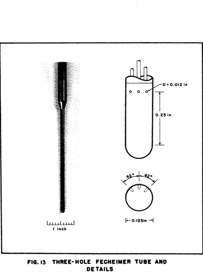
The type of probe used in all the measuremefits is shown in Fig.

13.

The probe is first yawed, using the two extreme holes, in the normal

fashion. The stagnation pressure

may then be read from the

center tap.

At the same time one may read1 the pressure indicated by either of the

ex-treme holes. This measurement, pi, when the probe has been properly

P -

Pi

pO

described in Ref. 25. The effects of turbulence on the readings were in all cases neglected.

These pressures were measured on null reading type transducer equipment manufactured by the Dynamic Instrument Co. of Cambridge, Massa-chusetts.

RPM was measured with an electrical strobotac.

All measurqments were taken at the mean geometric radius of the flow annulus.

The size of the perturbations may be represented by the ratio (U T )max. This value was of the order of .35 for the present series

of tests. The theory essentially neglects the third term in the expan-sion of

2

~

(+ !!) 2= 1 + 2 Mu + (u)2

U U U

The first term represents the mean condition; the theory treats the second term. The ratio of the term neglected to the term retained is thus at

2

most ₌

_.175.

4. CONPARISON OF THEORY AND EXPERIMENT

As explained previously, a knowledge of the upstream flow

(H/U2), _{the mean flow, and the rotor characteristics enables one to} solve for the perturbations everywhere. _{As the theory indicates, the im,}

portant perturbations are

6?/ot

All of these quantities were determined experimentally and the comparison with the present theory and that of Rannie-Marble are presented

in Section 4.2.

Another means of comparing _{the theory of Rannie-Mgrble with the}

present theory is through their respective predictions of tpe

perturba-tions in force on the blades. The present theory 4ttompts to correct the previous work by means of a more adequate prediction of the blade

load-ing. As has been noted one may compute the Rann e-parble prediction of

blade force, using equation 22.

As has been daiscussed, in the present theory one first finds ur an(% v, using the Rannie-Marble solution as a first approximation. The respective Isaacs and pears forces are calculated for this distur-bance flow. Then, applying these forces ia the present theory the

zec-ond approximation of the flow is obtained.

The above mentioned, forces were computed for each of the ex-periments conducted and the results are shown in Fig. 14-1 through 14-4.

It is also interesting to investigate by experiment the !valid-ity of the assumption tank ₂ = constant. This was done for a singie case

4.1 Comparison of Blade Force Predictions

The perturbation in y-component force on the blade, as discussed

in Section

4,

is shown in Fig. 14-1 through 14-4. The conditions of the

experiment are indicated in the cpgption.

No experimental data concerning

blade forces were taken. The non-dimensional values of the Sears and

Isaacs "forces per chord length" per unit span are shown as the two

bot-tom curves.

_{The next higher curve is simply an algebraic addition of the}

two aforementioned curves, hence it is also

a non-dimensional graph of

"force per chord length" per unit span. All of these three previously

mentioned curves apply to a single airfoil passing through the

distor-tion. If we multiply the middle curve by the chord pitch ratio, 2b/s,

we find the non-dimensional "force per pitch" per unit span and if we

then multiply by A, the lattice coefficient (Appendix V), we finally

find the non-dimensional "force per pitch" per unit span of an airfoil

in cascade. Thus we achieve the solid curve at the top of the figure,

which is compared with the Rannie-Marble prediction (2b/s

)

dashed curve, for this quantity. Note that the relative

size of the

Sears and Isaacs forces is related to the mean incidence, im. From

the theory, the Isaacs force

=

0 if

i is zero. This is of course not

true for the Sears force.

In general, the present theory predicts lower maxima and

higher minima than the previous theory.

4.2 Comparison of 9.1

6

A'

The perturbations upstream and downstream of the rotor as

ob-tained from the experiments and as predicted from the previpus theory

and the present theory are presented in Fig. 15-1 through 15-4. The

H

/U2

The present theory corresponds more closely to the experimental

data for all of the dowhEltream perturbations

(

/-

/

H2/U2) in each of the four experiments. The theory of Rannie-Marble

ap-parently offers a closer correspondence for the upstream quantities,

and . _{One should bear in mind several pbints, however, when}

comparing theory and experiment.

One factor is the ease with which 00 are "located" on the compressor, compared with the difficulty of establishing the points 0.

-27TX

This stems, of course, from the manner ( (Z ) in which the funda-mental harmonic of 0 and /'Pdecay with distance from the rotor. Thus

x-mislocation of a given amount has a larger effect on this factor for small x than for large x. Actually, if one places the actdator disc at

the half chord position this exponential factor for either the +0 probe

2n 1.5

or the -O probe becomes e - 1 2 = .645. That is, on this basis, 10.27 ( a

the theoretical curves for 6/ Oz/U 6

/U~and

are to be multiplied by .645 for a somewhat fairer comparison with

ex-periment. _{As may be seen, this tends to improve the correspondence}

be-tween experiment and both theories.

One would thus perhaps look to H2 A? as the most genuine

com-parison quantity for theory and experiment. It may well be, but again

the fluid is assumed inviscid, the perturbation in stagnation pressure is carried undiminished by the main flow. The experiments are, of course, conducted with a fluid of finite viscosity and the gradients are all di-minished by viscous decay. This is perhaps the reason for the

"under-estimation" of the attenuation of H by both theories. As is noted in the theory then, H_,

/U

/U2.

these quantities is made in Fig. 16. The downstream data tend to verify

the above discussion, though the upstream measurements do not allow one to make this conclusion.

Another point is that in the computation of both theories rela-tive stagnation pressure loss through the blade row was taken to be zero. Both theories do allow for finite losses and, as shown in Ref. 26, the in-clusion of this factor does in fact bring theory and experiment into closer correspondence.

4.3

The effect of flow rate on the attenuation is shown in Fig. 18. The experiment strongly indicates, for this case, larger attenuation at the lower flow rate. The theory of Rannie-Marble clearly indicates the

opposite trend. _{The present theory -agrees with experiment at least in}

several y intervals and clearly must be considered as predicting the

ex-perimental results more adequately. Perhaps the agreement would have been

further improved if an appropriate non-zero loss coefficient had been as-sumed for each flow rate. The lower flow rate curve could be associated with a higher 0_{D, perhaps giving more attenuation (Ref. 26) than that} re-sulting from the application of the smaller CD to the high flow rate

curve.

The effect of varying solidity on the attenuation is shown in

Fig. 19. Experiment indicates increasing attenuation with increasing

chord/pitch. This trend is also predicted by the present theory, though

the effect is underestimated. In this respect note that, since the blades

are unstalled, increasing solidity implies a higher loss coefficient CD

for the

_{higher solidity case. Referring}

_{again to Ref. 26, we infer then}

that if an appropriate C is used in each case, the higher solidity curve

D

will receive more attenuation than the lower solidity curve, improving

the prediction of the effect of solidity. The Rannie-Marble theory of

course can offer no information on this effectA since their theory treats

only the single solidity 2b/s

=

o

_{Note that, because in the experiment,}

the attempt to keep flow rate constant at eaqh solidity was not successful

(there being no convenient means to control this parameter for the

dis-torted

_{flow except by measuring a representative velocity) one had to}

in-terpolate between flow rates, as indicated on this Figure.

,It

_{should be noted that, as is to be expected, the curves of H1/32}

5.

CONCLUSION

A theory for asymnetric inlet flow in an isolated blade row has

been _{developed. This theory gives a prediction for distortion attenuation,}

effect of flow rate, and effect of solidity variation which agrees more

closely with the present experiments than does the previous theory. For the cases tested, attenuation was increased by reducing the flow rate and by increasing the chord-pitch ratio,

The attempt to improve the prediction of blade forces

thus appears to have been a fruitful approach to the problem of asymmetric

inlet flow. In particular, the effect of velocity perturbations in the direction of the mean relative velocity vector, often ignored, is seen to be the dominating influence at the larger values of mean incidence.

APPENDIX I

A Boundary Relationship Between Two Cauchy-Riemann Variables

Since the two velocity components (u, v) in plane potential flow

c.44 .W

r

satisfy the Cauchy-Riemann conditions ( + .O ---

=0

ax~~~ ay > T C

it will be convenient to derive the. following in terms of these variables. It is understood, however, that the following is true for _an pair of Cauchy-Riemann variables.

Let u be periodic along the y axis of period 1, and let this ve-locity distribution be the result of a source distribution along the y axis, also of period 1, Figure A - ... That the introduction of the sources does not make the following less general follows from the second fundamental

theorem of potential theory: if continuous boundary values are assigned,

on the surface of a regular region, to the normal derivatives, not more than one function, apart from an additive constant, harmonic in the region,

can have normal derivatives with these values. For infinite regions, we

require that our harmonic function (in this case the velocity potential

q1

)

be regular at infinity. That is, 14 / shall be bounded in

absolute value for all sufficiently large r, where / is the distance from

any fixed point. That is, thus far all we have assumed is that u is

peri-odic along x = 0, period = 1, and that the velocity potential 9 is

regular at infinity. Our results will hold whether this periodic

2

/

cit

~'z4

Ii

o0

(XJ

'*/)

x

1

Tkhe source strength 0V of an element is clearly 2,ad₇

.

In the following, /7 X

/

shown in Figwre A - 1 and the elements at 1/2)) , .,

t ?)

-2 -'7)

4 -/.~/ ,,[ 7-I/-f)-lthat is, corresponding elements in the wave length.

Let be the complex potential at z due to the sources at these

loca-tions. 2rl t."

-]]

L

71

f,

In

(:E-

)+/-n

7n')

)J

/7f

71-

_/_

-

7,

Qe)

The last term, 14

77'

alq-

0

0,1W)/

The infinite product has a special form :

/

--

(Z

Log

-s-

Nw, _{to find the influence of} all the sources, we mast integrate

from 0 to 1.

-~

ca

Z7T/J/k/}

7/

-i ?)/t

And finally we find

-

f

/

t

0('

-

V

)

=

-f

Zr

Specializing to z on the y axis

r

=--

77

(Y

)

-Q

7

/7

-

(

Suppose that x = _{0 is a line of discontinuity (as, for example,}

in actuator disc theory). Now we consider properties at x = 0+ and at

x = 0-. For the region x > 0, _{since we have assuued that dQ is a source,} and hence > p 0, &Q 2 =

al

)

)

u \ 0 for x =0-, Figure A.,L, for the region x ( 0 we 'have dQ = -2AAd.

Note that, frm symetry,

VT

(~

*

y)o=

ZT(X

?)

?rIo-,

y) =

-(0

cct

9'-7)J

(0

-,

/

~ ₀

C6

mainple

Given u(O+, y) = C, a, constant

Then ?y(0't/= _C

Then)

74~

I

APPENDIX II

u,

v,

3

/1)

Con-ditions to RIlations in /qj

The defining equations for (JP (9 are

/f,

+IL

=

A/

VAx +zr = 0

Regarding this as a set of three linear algebraic equatigns, may solve for u, v, and p successively. One then finds that

A2-1

A2-2

A2-3

Then, whenever u, v or p/p appears in a boundary condition we

substitute the expressions given above. This operation and the result-ing simplifications are set forth as is shown.

The matching condition u₂ = u1 beccmes

letting

v

U

A2-5

For the Bernoulli equation with losses, we have

-f/p

V(-a

r)-zf

/

4z

(Vz-ar

)+,

,

C

Cos

2-(0,-1ard,)

Translating into

A'

6~7 ~(~-6'-

*

,

;2, Gt,Q

"

J, P

C-p

2C0,5

9m

-

L,

Y20-(V -.

12

)

--n

~~r)

U(Vz

IL+

izr)

V

("V,

_ (Vz -(2 r)

~

'7L+VI

U

2~

W,~

L2

P1

V2

t'

U7-+,L

&:>

6os5

zcek

₆

6

Lg)

6%4

~

S 7

,4

UV

2-7Y//

_{P7(Q - 6P2)}

62_ 70Le // -2) ,

letting

4

7

Z

we finally obtain

6>

-

5C

-

J I)

fp7

9

=6e

e

*

(//

_-6)

6z

)

For the tangential momentum boundary equation, we have

=

(v--

)

_t2(VI-Vz)

=

L(&5;,-r)ta

(V.-V)-z

=

U

h,-

)

(v.-V)+z

=

U(Z;-

r

)

-Vj)2

7C)

+V;-;

V

tu

)itt

euy

(

-

(UU

-V/

A~

e,

/-97-

_{z ces,}

₎

A2-7

A2-6

Z

v

-UNve

/

UN v

)

U

,

vj

U -7

=

U

ZT

-

-

e - 0/ an 0/

Tabulation of tie

U

S

V

vz

Ut

2

v-~

-i r)

V,-v, ( -2. r)

u(v

--

ar)

el

=

z

coSe.0

00

-2n-

)

/In

LrevLK

z CosL(Vn

.,r

u"V,

~/7

UV/

V

11/

t

l

V-.,r

~. U

7 ,'v

V'

U

SC5 /I

C7

_~k

v,2

vnW

a

_

V7,-

v.-ar

5t=

U

2

_U

_u#'+

v,

(v,-Ar

)

U~

/

.'v

2

U

cos

Ln

v.(v-Y2r)

?ZC

=

/-

zces

69l

(7'e6

)

-

z

t9,

e;%.

f,=

ei

~/

2 2-____ (

5 ?Z73

27

ri-()-(Zre

U--

r)_

vU

C

+

s

Ccs

CD/cZS?/;rn

Z s,

W(V2-.2

Z,

L7Qr

APPENDIX IV

Description of the Computation (Programming)

The present theory was programmed, not as a unit, but rather as a main program and two auxiliary programs. The divipion exactly follows

the development in the text. That is, the main body of the theory, con-sisting f tbe operations indicated in Section 2.3 exists as the main

pro-gram. Both the Sears force and the Isaacs force occur as separate pro-grams whose output, when operated on in the manner described in the test, serves as partial input for the main program. A description of these pro-grams, together with sample or 'test' solutions appears as subsections of

this appendix.

The computer was the M.I.T. Computation Center IBM 704 Electronic Data-Processing Machine.

A4.1 Main Body of the Present Theory

The block diagram for the computation is shown in Fig. 20.

Each instruction is of course not listed but rather the 'general manner in which the computation proceeds is indicated.

The input information for this program is: a) 51 y-equispaced values of H₁

b) 51 y-equispaced values of

c)

9

constants

z

.

7'

?

y S

The output information is 51 y equispaced values of each of Os,

6

find-02.)

62 a

algebraic equations, it is easy to see that an alternate set of input in-formation is a) 51 y-equispaced values of H/ b) 51 y-equispaced values of A - -f SU 2 7

c)

9

constants

A

07> 8

i

?'7>

zc

With this input, the output information is 51 y-equispaced values

of

%2.

The latter method

was actually used. As indicated, the program stops after the last (y = 1.0) set of output is printed.

As is customary in machine camputation, one checks to see that the programming is correct by using the program on a non-trivial problem whose answer is known, from hand computation or elsewhere. For this

pro-gram the test solution was exactly the case illustrated in Fig. 26. The

required blade force information, labelled (b) above was artificialy

sup-plied from a previous Rannie-Marble solution:

DSz

z

~$

Z. +-

;92

Therefore the test solution should be exactly that given in Fig. 26. This was the solution achieved.

A4.2

Sears

Force

vr(y) is first detemined from Rannie-Maxble solution as follows:

~

10/(--

₀

Vi

C2

)

S2fv

T-

4

o

(

t)]

=f za~s'4

~~1

_+C-

_C

_O

_S

U.

*L

V

Cosni

The mathematical statement of the problem may then be written

CvS2 7Pmf)

A4.2-1

.4/0

b

ifCSrM

S(nl,

00

Let us let

Recalling that

6.4,,=

2

C2.

-Z2

Zn11

we then have, from A4.2-2,

277 i-S,.-r) (Z X4,/ -/-3n Then 061L

A4.2-2

= 2

~~z

However, it is not possible to represent by a cosine series such as A4.2-1 which has common period 1, a general function whose period is 1. Rather, to represent a function of period 1, we need cosines of common wave length 2.

Therefore, if we represent vr(y) as

Ur y

)=

2

C6on

7/

t=0

the force expression will be given b

A4.2-3

z X7

s

zl

b7rWr

COs

>

~z

A4.2-4 becomes

C6s

(701

2

T

Wr is in general -.. XL The fundamental non-dimensional fre-quency is

In the present experiments, the physical fundamental wave length was yR. However as previously discussed, the computation is carried out

with twice this fundaniental period. therefore, for computation purposes,

__

_

The input for this program was thus

a) 51 y-equispaced values of vr(y)(vr(o) ... vr(l))

b) 27rJ2.

c) AVOcosM

The output information was 51 y-equiipaced values of -The test solution for this progam is shown in Fig. 22. Twenty harmonics are used in the ccmputation. As indicated in the block diagram, the values

of An and Bn, indicated in A4.2-5, and characterizing the Sears function, were stored in memory and located, according to the frequency of the

parti-cular harmonic; by a table interpolation subroutine.

A4.5 Isaacs Force

ur(y) is first determined from the Rannie-Marble solution as follows:

2&T

a

cos

,? -O/(/$5)#(

-

?SLos ji)

.#U_6

j

t

-

v

(i-6)+U

2.

C05

~

_

-_.___

V

1]

V&7-We have seen that for

~

A

q,/

t$I

k4~

I

4=1

COS O

6/1

Z

7/X

If, on the other ha4,, ur is represented as

00

then

--

h

En

cs

9

b, wt

then the force could be written

7.4

En

(4;

r1f 54 1 M V7C IO

-6

5w~, U'

For present purposes, /,

27rt2

(b/A)

JLttr

2

Ar)

A0

+

V~b

_-?m~c731)nz

(L/'I

Y)L

Cvsz5rnXM1

-L

z

L2

7

/

9-I

+ CoS4-T4X

zxb)Z~rn

2.

51n

7F~X

I1

CO52.nie

t

I

;3-b

, O

z

n!

Si)fid. |

fn

6Jr-udr b

,a ,r

2

n=/

E,7 Cs

0, Z />4

Z-Then if the ur representation is

/2=1

F

L

(

511/

2M71/

-Ei

co,527rny

2

₂

144

E,

-

2

,s

dr

the force perturbation will be

=0 _s

IT-51tIM~a

(

7

2/12

2-

.r,

O

Cs

z7T/Y

)sii

T f

QP4) Z)

s'rZ77My

_{)Z)Cosz Iy*}

En

l

_Til

_,5

i

ivr>y+~

z

ii

9/1/

tr

_{z ovn}

)

I

/kpi

)

-.

P

,/7

₂₄₂

_C054IT4y

0

Z,

.ar

(L'i/+