Biophysical responses of lymphocytes to environmental stress

Biophysical responses of lymphocytes

to environmental stress

by

Vivian Hecht

B.S. Bioengineering, University of California, Los Angeles (2010)

Submitted to the Department Of Biological Engineering in Partial

Fulfillment of the Requirements for the Degree of

Doctor of Philosophy

at the

Massachusetts Institute of Technology

February 2016

C Massachusetts Institute of Technology. All rights reserved.

Signature of Author...

Certified by ...

Accepted by...

Signature redacted

September 17, 2015

Signature redacted

Scott R. Manalis

Professor of Biologica) and Mechanical Engineering

Signature

MAY 2

6

2016

LIBRARIES

Thesis committee members in favor of defense:

Professor John Essigmann

Professor Matthew Vander Heiden Professor Scott Manalis

Biophysical responses of lymphocytes

to environmental stress

By

Vivian Hecht

Submitted to the Department of Biological Engineering On September 17, 2015, in partial fulfillment of the

Requirements for the degree of

Doctor of Philosophy in Biological Engineering

Abstract

Cellular biophysical properties both reflect and influence cell state. These

parameters represent the consequences of the interactions of multiple molecular events, and thus may reveal information otherwise obscured when measuring individual pathways in isolation. Previous work has demonstrated how precise measurements of certain of these properties, such as mass, volume, density and deformability using a suspended

microchannel resonator (SMR) can help characterize cellular behavior and physiological role. Here, we expand upon this previous work to demonstrate the necessity of measuring multiple parameters simultaneously to fully determine cellular responses to environmental perturbations, and describe a situation in which changes to density and size promote

survival under conditions of limited nutrient availability.

We first investigate the relationship between cell density, volume, buoyant mass, and passage time through a narrow constriction under a variety of environmental stresses. Osmotic stress significantly affects density and volume, as previously shown. In contrast to density and volume, the effect of an osmotic challenge on passage time is relatively small. Deformability, determined by comparing passage times for cells with similar volume, exhibits a strong dependence on osmolarity, indicating that passage time alone does not always provide a meaningful proxy for deformability. Finally, we find that protein synthesis inhibition, cell cycle arrest, protein kinase inhibition, and cytoskeletal disruption result in

unexpected relationships between deformability, density, and volume. Taken together, our results suggest that measuring multiple biophysical parameters can detect unique

characteristics that more specifically reflect cellular behaviors.

We next examine how cellular biophysical changes occurring immediately after growth factor depletion in lymphocytes promote adaptation to reduced nutrient uptake. We describe an acute biophysical response to growth factor withdrawal, characterized by a simultaneous decrease in cell volume and increase in cell density prior to autophagy

initiation, observed in both FL5.12 cells depleted of IL-3 and primary CD8+ T cells depleted of IL-2 and differentiating towards memory cells. The response reduces cell surface area to minimize energy expenditure while conserving biomass, suggesting that the biophysical properties of cells can be regulated to promote survival under conditions of nutrient stress.

Acknowledgements

I would first and foremost like to thank Professor Scott Manalis for his guidance and

mentorship during the course of my thesis work. His dedication and enthusiasm helped me succeed and I am very fortunate to have had the chance to work with him. My thesis committee members, Professors John Essigmann and Matthew Vander Heiden, were sources of valuable feedback and perspectives regarding the progress of my work. I would also like to thank Matt for sharing his biological expertise in the area of growth factor dependence in lymphocytes, as well as providing me with the opportunity to collaborate closely with his lab.

Next, I would like to thank the members of the Manalis lab, past and present, an exceptionally talented group of individuals who made for truly excellent colleagues. Andrea Bryan, who trained me when I first arrived, set an excellent example for me and has

continued to be a mentor and friend since then. Will Grover continually encouraged me and helped me troubleshoot the dual SMR. Will and Andrea together pioneered the SMR

density measurement, enabling me to use the method to answer the biological questions addressed in this work. Sangwon Byun's thoughtful and careful approach to the

deformability and density project were essential to its success. Edgar Aranda-Michel and Kevin Hu contributed both their image processing talents and positive outlooks, generating sufficient momentum to push through the challenging periods of developing the affinity chip. Josephine Bagnall was a source of both technical and moral support, and I was very happy to have her as a teammate in the ladies' section during lab meetings. Selim Olcum and Nate Cermak demonstrated unwavering patience and dedication in ensuring that my SMR setup function properly, and always found time to help me identify issues with

electronics in spite of being constantly bombarded with questions from other lab members.

Scott Knudsen was a constant source of a wide breadth of useful and entertaining

knowledge, and I am indebted to him for both solving many SMR-related problems and

sharing with me fascinating science trivia. Mark Stevens and Rob Kimmerling provided

invaluable biological guidance as well as comic relief; Rob's input during the affinity chip

project was tremendously helpful.

I am also grateful for the support of multiple collaborators. Lucas Sullivan served as

a translator and guide through the fascinating and often confusing depths of mammalian

cell biology and metabolism. Dong-Hwee Kim's imaging expertise provided a useful

complement to our biophysical measurements. Greg Szeto was always willing to share his

encyclopedic knowledge of immunology, and provided invaluable support during the affinity

chip project.

Finally, I would like to thank my friends and family for their continued support

during the course of my thesis work. My parents, who encouraged me from the very

beginning, and always reminded to persevere no matter how seemingly difficult the

challenge. My older brother, Ariel, first introduced me to microfluidics, and set a stellar

example for me to follow; my younger brother, Avi, was always willing to listen to any of my

concerns and propose the most reasonable solution. And last of all, I would like to thank

my husband, Aaron, whose kindness, patience and sense of humor made this entire work

Contents

Chapter 1

Introduction ...

19

1.1

The interplay between cellular composition and behavior...19

1.1.1 Methods for determining size and composition...21

1.1.2 Single-cell density ... 23

1.2

Measuring density with a suspended microchannel resonator...24

1.2.1 Principle of operation ... 24

1.2.2 Single and dual cantilever methods for measuring density...29

1.2.3 Approaches for minimizing measurement error ... 41

1.3

Approximating the effects of changes to cellular composition on cell

den sity ...

. 4 9

Chapter 2

Characterizing cellular biophysical responses by relating

density, deformability and size ...

53

2.1

Introduction ...

53

2.2

R esu lts ...

. 55

2.2.1 Characterizing the density and volume of cells exposed to osmotic stress...55

2.2.2 Characterizing the passage time and deformability of cells exposed to osmotic stress. 59 2.2.3 Characterizing cell states by deformability, density, and volume...64

2.3

Conclusions...

68

2.4

M aterials and methods ...

69

2.4.1 Cell culture and preparation... 69

2.4.2 Experimental systems... 70

2.4.3 D ata an alysis...73

Chapter 3 Biophysical changes reduce energetic demand in growth

factor deprived lym phocytes ...

75

3.1

Introduction...

75

3.2

Results ...

77

3.2.1 IL-3 depletion results in both atrophy and density changes in FL5.12 cells.... 77

3.2.2 Autophagy and IL-3 depletion lead to different biophysical changes...82

3.2.3 Biophysical changes allow adaptation to decreased nutrient uptake...84

3.2.4 IL-2 depletion in primary T cells leads to changes in density and volume ... 87

3.3

Discussion...

90

3.4

M aterials and methods ...

92

3 .4 .1 C ell cu ltu re ... 9 2 3.4.2 Confocal microscopy and high-throughput cell phenotyping ... 93

3.4.3 Immunoblotting... 94

3.4.5 Mitochondrial oxygen consumption... 94

3.4.6 Metabolic measurements ... 95

3.4.7 Statistical analysis... 95

Chapter 4 A microfluidic approach for characterizing lymphocyte

avidity interactions...

97

4.1

Introduction...

97

4.2

Device design...

101

4.2.1 Eight port configuration...101

4.2.2 Four port configuration...110

4.2.3 Modeling APCs with functionalized beads ... 113

4.3

Results ...

114

4.3.1 Experimental workflow...114

4.3.2 Data analysis...116

4.3.3 Preliminary results ... 119

4.4

Conclusions and future work ...

123

4.5

M

aterials

and m ethods ...

125

4.5.1 C ell cu ltu re ... 125

4.5.2 Bead synthesis...126

4.5.3 C ell stain in g ... 126

List of figures

Figure 1.2-1. Calculating single-cell mass, volume, and density. ... 26

Figure 1.2-2. Calculating single-cell dry mass, volume, and density. ... 27

Figure 1.2-3. Schematic of the single SMR density measurement... 32

Figure 1.2-4. Diagram of the fluidic and pressure components in the single SMR. 33 Figure 1.2-5. Changes in density values over the duration of a measurement... 33

Figure 1.2-6. Schematic of the dual SMR measurement. ... 35

Figure 1.2-7. Diagram of fluidic and pressure components in the dual SMR. ... 36

Figure 1.2-8. Comparison of different dual SMR channel designs. ... 38

Figure 1.2-9. Measurement uncertainty as a function of Fluid 2 density in the case of purely m ultiplicative error... 42

Figure 1.2-10. Measurement uncertainty of cell density or cell volume is a function of Fluid 2 density in the case of purely additive error... 43

Figure 1.2-11. Measurement uncertainty of cell density and cell volume as a function of Fluid 2 density, assuming no uncertainty in measuring fluid density.. 44

Figure 1.2-12. Comparing the effects of additive error when measuring total density and dry den sity ... 46

Figure 1.2-13. Cantilever mode shape and peak shape in first and second modes.. 47

Figure 1.2-14. Comparison of distributions of 10 pm polystyrene beads measured in first mode with a dual SMR, and 8 gm polystyrene beads measured in second mode w ith a sin gle SM R . ... 49

Figure 1.3-1. Relating changes to biochemical content to changes in density... 51

Figure 1.3-2. Relating changes in aqueous content to changes in total density. .... 52

Figure 2.2-2. Effect of osmotic stress on passage time and buoyant mass... 60

Figure 2.2-4. Estimating error associated with converting buoyant mass to volume

using a density m easurem ent. ... 63

Figure 2.2-5. Deformability versus density and volume for various conditions... 65

Figure 2.4-1. Cell density versus volume of FL5.12 cells treated with STS. ... 71

Figure 2.4-2. Schematic diagrams of the approaches that measure deformability

and examples of the data extracted from the measurement... 73

Figure 3.2-1. IL-3 depletion leads to a decrease in volume in FL5.12 cells over a 120

h p e rio d ... . . 7 8 Figure 3.2-2. IL-3 depletion leads to a decrease in density and dry mass in FL5.12

cells over a 120 h period. ... 79

Figure 3.2-3. High throughput cell phenotyping (htCP) performed on control cells

and 120 h following IL-3 depletion... 80 Figure 3.2-4. Biophysical changes to FL5.12 cells upon IL-3 repletion (black arrow)

follow ing 120 h of IL-3 depletion... 82 Figure 3.2-5. The biophysical response of FL5.12 cells to autophagy induction... 83

Figure 3.2-6. Short term changes to FL5.12 volume and density following IL-3

d ep letion ... 8 4

Figure 3.2-7. Changes in FL5.12 metabolism following IL-3 depletion. ... 87

Figure 3.2-8. Biophysical responses of CD8+ OT-1 cells 72 h after activation with

continued exposure to IL -2. ... 88

Figure 3.2-9. Biophysical response of CD8+ OT-1 cells to growth factor depletion. 89

Figure 3.2-10. Biophysical to FL5.12 cells following exposure to IL-15. ... 90

Figure 4.2-2. Diagram of fluidic and pressure components in eight port

con figu ration . ... 10 4

Figure 4.2-3. Experimental workflow for eight port design. ... 106

Figure 4.2-4. COMSOL modeling of fluid flows through the main flow channel....109

Figure 4.2-5. Schematic of four port design for measuring cell-cell avidity. ... 111

Figure 4.2-6. COMSOL modeling of flow through a single turn in the serpentine channel of the four-port design...112

Figure 4.2-7. COMSOL modeling of fluid flow across channels in four-port design. ... 1 1 3 Figure 4.3-1. Loading beads into traps...115

Figure 4.3-2. Observing cell passage through channels loaded with beads...116

Figure 4.3-3. Data processing method for measuring cell velocity across the serpentine trap ch annel...117

Figure 4.3-4. H istogram s of cell velocity ratios. ... 119

Figure 4.3-5. Velocity ratios per lane over the course of an experiment. ... 120

Figure 4.3-6. Absolute velocity over time in individual lanes...122

Figure A.1-1. A pre-apoptotic signature observed in multiple cell types under a variety of con dition s. ... 13 1 Figure A.3-1. Volume vs. dry mass of multiple adherent and suspension cell lines an d p rim ary cells...135

Figure A.3-2. Fractional water content (by volume) vs dry mass of multiple adherent and suspension cell lines and primary cells. ... 136

Figure A.3-3. Fractional water content (by mass) vs dry mass of multiple adherent and suspension cell lines and prim ary cells. ... 137

List of tables

Table 1.2-1. Expected and measured values of osmolarity of Optiprep solutions at a

ran ge of concentrations... 30

Table 2.2-1. Biological effects and mechanisms of drugs used in Figure 2.2-5. ... 66

Chapter 1

Introduction

1.1 The interplay between cellular composition and

behavior

Cellular composition, describing the relative amounts of all intracellular

biomolecular components, is a parameter often predicated upon physiological role. For

example, adipocytes, which serve primarily as lipid storage centers, have a high fraction of

triglycerides and cholesterol esters. Conversely, myocytes, the cells comprising muscle

tissue, contain high levels of glycogen, a readily accessible source of energy, and

mitochondria, for generating ATP. As the need for space for energy storage or strength

changes, the composition of these cells will adjust accordingly.

In other cases, however, cellular composition can influence specific cellular

behaviors. For example, the hormone insulin, released due to elevated blood glucose levels, stimulates cellular ion channels to increase water uptake (1, 2). This increase in cell water

content leads to an increase in cell volume that has been shown to upregulate anabolic

processes, such as glycogen synthesis, and downregulate catabolic processes, such as

gluconeogenesis. Glucagon, released when blood glucose levels decrease, causes the

certain neurodegenerative diseases, including Alzheimer's disease, Parkinson's disease, Huntington's disease and amyotrophic lateral sclerosis, are characterized by accumulation

of protein aggregates in various categories of neuronal cells. These protein aggregates, caused by stochastic processes, aging, or overexpression of genes responsible for synthesis

of specific proteins, tend to overwhelm the native cellular protein degradation machinery

(3).

The close relationship between cellular composition and cellular behavior suggests

the need to tightly regulate composition to ensure the proper function of cellular machinery.

This is made especially clear when considering the significant level of cytoplasmic

macromolecular crowding (4). Shifts in concentrations of both macromolecules actively

participating in reactions and bystander or inert macromolecules can influence cellular

reaction rates and protein equilibria (5). For example, while a higher level of crowding will

lead to a decreased reaction rate in diffusion-limited reactions, it will also increase the rate

t pt i t

misfolding diseases have been shown to be more likely to form aggregates with increasing

total cytoplasmic concentration (6).

To more completely characterize a cell from a biophysical standpoint, its cellular

composition must be considered in the context of its size. Size can be described using a

variety of parameters, including volume, mass, and buoyant mass (i.e. the mass of a

particle measured in a fluid). One of the most fundamental reasons for changes to cell size

is progression through the cell cycle, as cellular macromolecules, organelles, and genetic

material must be replicated to provide sufficient material for two viable daughter cells.

This results in an increase in size until a division event; however, whether any changes

type (7, 8). Increases in size caused by physiological need rather than cell cycle stage also

occur regularly in certain cell types-for example, kidney and bladder cells will swell or

shrink due to changes in water uptake, to maintain an appropriate systemic osmolarity.

During apoptosis, certain cell types will undergo changes to volume, likely driven by

changes to water content, prior to blebbing and membrane permeabilization (9, 10).

Furthermore, lymphocytes will increase in size following activation, and decrease in size

during the process of differentiation to memory; the changes to composition that are

associated with this process are discussed in greater detail in Chapter 3.

In spite of the significant role that composition and size play in cellular function, many studies disregard these properties in favor of focusing on individual molecular

pathways. However, a significant fraction of physiological events occur as a result of the

contributions of and interactions between multiple pathways, not all of which can be

identified a priori. Because composition and size are by nature aggregate parameters, they

can, therefore, reveal information about cell state that is obscured when considering

individual pathways in isolation.

1.1.1

Methods for determining size and composition

Perhaps the most rudimentary method for determining cellular composition is with

direct mass measurements. This technique, still commonly practiced, involves weighing a

cell pellet with a previously quantified number of cells, drying the pellet in an oven for

24-48 h, and finally weighing the dried pellet (11). The dry mass and water content per cell

can then be calculated. However, this approach is time intensive, limited-in precision, and

unsuitable for identifying any subpopulations or individual outliers in a sample.

applying the technique to rare samples. Furthermore, the substantial amount of cell

handling can stress the cell sample and introduce biological artifacts. Finally, once the

cells are measured in this method, they are no longer viable and cannot be grown further

and analyzed with downstream experiments.

Measuring composition and size with microscopy overcomes many of the

shortcomings of direct mass measurements. Particularly useful is interferometry, a

microscopic technique in which the phase shift between the wavelengths of two beams of

light-one a reference and the other emitted from a sample-is used to obtain information

about the sample. This phase shift is caused by a difference between the refractive indices

of the reference and the sample. The refractive index in cells is directly proportional to

biochemical content, or dry mass; thus, with interferometry, the dry mass of cells can be

precisely quantified (12-14). Interferometry has also been used to determine changes in

water content of kidney cells (15). More recently, this technique has been adapted to

dynamically ouantify changes in dry mass of growing eflls (1 6). UIing th onticallv

calculated volume and dry mass, a dry mass density can be obtained; this is a measure of

the amount of dry mass per total volume. However, interferometry cannot be used to

determine absolute water content, and it does not provide information about the

composition or chemical makeup of the dry mass. Furthermore, this technique relies on a

constant refractive index for all biomolecules in the cell; this assumption holds true for

most proteins, but is not always valid for carbohydrates and lipids (17).

Raman spectroscopy, an alternative technique, has proven to be particularly

well-suited for determining the chemical composition of cellular dry mass. The method involves

illuminating a sample with a monochromatic light source, and measuring the scattered

caused by some fraction of the light interacting with the bonds in the molecules of the specimen. The nature of these interactions depends on the identity of the atoms in the molecule and their arrangement in bonds; thus, the spectrum of frequencies reflects the structure and composition of the molecule. Classes of biomolecules are characterized by specific functional groups, and so the peaks that appear in a Raman spectrum can be traced back to their biomolecules of origin. A stronger signal at a given frequency, represented by a larger peak, suggests that the molecule is present in a greater amount.

In general, however, Raman is best suited for comparative analysis, or for

determining the structure of single proteins and molecules; obtaining precise, quantitative values for the total dry mass in a cell can be challenging. Another feature of Raman spectroscopy is its weak signal from water (18, 19). Consequently, any water in a sample will not interfere with signal acquisition of chemical components. However, this limits Raman to measuring biochemical components exclusively, and precludes it from use in determining cellular aqueous content.

Recently, a method has been developed which combines Raman spectroscopy with quantitative phase microscopy, allowing for simultaneous measurement on a pixel-by-pixel basis of the morphology of a cell and its chemical composition (20, 21). This method allows for simultaneous size and composition determination, with a high resolution of information in both. However, this high resolution limits the throughput, rendering the technique suitable for only specific applications.

1.1.2

Single-cell density

We focus on the application of cell density, or the ratio of cell mass to volume, as a proxy for cellular composition. Density reflects the combined contribution of all biochemical

components and water; while density, independently of other metrics, cannot be used to determine the amounts of individual components, it can be used to differentiate between populations of cells, and changes to density typically suggest changes to cellular

composition. Previous studies have shown that density can be used to identify circulating tumor cells, distinguish among different populations of liver cell types, differentiate between proliferating and non-proliferating cells, and differentiate between healthy and diseased red blood cells (22-24). Here, we demonstrate the application of density to address fundamental biophysical questions relating to cell state. We combine extremely precise measurements of density with those of volume, size, and deformability, and with orthogonal assays, to provide novel insights into cellular responses to environmental perturbations and nutrient stress, and propose possible biological mechanisms underlying the changes to density that we observe.

1.2 Measuring density with a suspended

microchannel resonator

1.2.1

Principle of operation

The SMR, or suspended microchannel resonator, is a cantilever-based mass sensor with an embedded microfluidic flow channel. The principles of its operation have been described at length elsewhere, and will be summarized here (25-30). The SMR consists of a hollow resonating cantilever flanked by two bypass channels. A cell is introduced from a bypass channel via pressure-driven-flow, and flows across the cantilever, changing the cantilever mass. The resonance frequency of the cantilever is based on its mass, and the event of a cell passing through will lead to a change in resonance frequency that is

monitored via a feedback circuit. This change in frequency corresponds to the buoyant

mass of the cell, or the mass of a cell in its surrounding fluid:

MB = mceii( -

L

Pceli

1.2-1.

where mB corresponds to cell buoyant mass, meell corresponds to total cell mass, pf

corresponds to the density of the surrounding fluid, and peesl corresponds to the cell density.

This equation can be rewritten to describe buoyant mass in terms of cell volume, Vei, as

well:

MB = Vcei (pceii - Pf

1.2-2.

The buoyant mass of a cell is related to the change in cantilever resonance frequency

via calibration with polystyrene beads of known mass, calculated from the diameter

reported by the manufacturer and the density of polystyrene (1.05 g/mL). Similarly, the

density of the measurement fluid can be determined with a calibration of fluids of known

densities, obtained here from solutions of NaCl in water. Thus, the total mass, volume and

density of a cell can be determined by measuring the buoyant mass of a single cell in two

fluids of two different densities (Figure 1.2-1). This method is based on Archimedes'

Principle, in which the eponymous philosopher determined the purity of a gold crown by

weighing it once in air and once in water, and comparing the result to pure gold weighed in

Y-intercept:y mass

*0

Figure 1.2-1. Calculating single-cell mass, volume, and density.

Cell buoyant mass is measured in two fluids of different densities (red and blue dots) to determine the linear relationship between buoyant mass and fluid density. The absolute mass (y-intercept), volume (slope), and density (x-intercept) of the cell can then be calculated.

1.2.1.1 Measuring aqueous and non-aqueous content

More recently, a method to determine additional information regarding cellular

biochemical content using the SMR has been developed (30, 31). Cells are measured with

the technique described in 1.2.1, though with PBS and D20-PBS (lx PBS in 90% D20) as

the low and high-density fluids, respectively (Figure 1.2-2). The cell membrane is

permeable to D20-PBS, and so when a cell is measured in D20-PBS, its aqueous content is

replaced with D20-PBS. This produces a buoyant mass measurement representative of the

buoyant mass of the non-aqueous material exclusively. Similarly, when the cell is

measured in PBS, we can approximate that the composition of the intracellular aqueous

content to be similar to PBS; thus, a buoyant mass measurement in PBS would also

represent the buoyant mass of the dry material. The cell buoyant masses in PBS and

This dry material includes lipids, proteins, nucleic acids, polysaccharides, and other small molecules. The interpretation of dry mass and volume is relatively straightforward-i.e. how much the biochemical content weighs and how much space it occupies. The dry density can be understood to represent the weighted average of the densities of the individual biochemical components. Thus, dry density can be considered a proxy for cellular biochemical composition.

Y-intercept:

dry mass uoyant

iass inl

l) _{Slope: dry volume}

E

0 X-intercept:

dry density

Fluid density (g/mL)

Figure 1.2-2. _{Calculating single-cell dry mass, volume, and density.}

Cell buoyant mass is measured in two fluids of different densities, both permeable to the cell membrane (red and green dots), to determine the linear relationship between buoyant mass and fluid density. The dry mass (y-intercept), volume (slope), and density

(x-intercept) of the cell can then be calculated.

Finally, by combining information from the dry density, mass and volume with that of the total (i.e. aqueous and dry) density, mass and volume, the aqueous content of a cell can be estimated. The procedure for determining this value has been described elsewhere, and is summarized below (30, 31).

We start by describing the total mass of the cell (mt,) as composed of aqueous

Mtot mwater + mdry

1.2-3

We can rewrite this equation in terms of density and volume, based on the general

relationship between mass (m), density (p) and volume (I0):

m=pV

1.2-4

PtotVtot

1.2-5

where ptot, pwater and pdr refer to the density of the total cellular, aqueous, and dry material,

respectively, and Vtot, Vwater and Vdry refer to the volume of the total, aqueous, and dry

material. We can also describe the volume of the cell in a manner similar to Equation 1.2-3:

Vtot = Vwater + Vary

1.2-6 By combining equations 1.2-5 and 1.2-6, and assuming a water density of 1 g/mL, we

can obtain expressions for the amount of aqueous material, described in terms of volume:

Vwater = Vtot

1

-(Pdry-1

1.2-7 If we continue using the assumption that the density of water is approximately 1 g/mL,

then the value provided by equation 1.2-7 also describes the total mass of water (mwater).

The dry density measurement is associated with a number of limitations. First, it is

susceptible to relatively high levels of uncertainty due to measurement errors, as discussed

further in 1.2.3.11.2.3. Additionally, the process of water/D20 exchange is not entirely

clear. Though the exchange occurs approximately instantaneously for mammalian cells,

whether all water is exchanged or simply free water in the cytoplasm remains to be

interpretation for changes to dry density, as the density of the individual components may

not be immediately obvious. Nonetheless, dry density may be a useful indicator of changes to cellular composition, and may be more clearly interpreted when combined with an

orthogonal measurement of chemical composition, such as interferometry or Raman

spectroscopy.

1.2.2 Single and dual cantilever methods for measuring density

Determining cell density by measuring the mass of a single cell in two different

fluids can be accomplished in a number of ways. The two which will be discussed here are a

single-cantilever method (32) and a dual cantilever method (33). Both methods involve

measuring a cell in a low-density fluid (Fluid 1), typically cell media, and a second fluid

(Fluid 2), which is a mix of a small part of cell media and a high density fluid. In initial

studies, Percoll, a suspension of silica nanoparticles, was chosen as the high density fluid,

due to its biocompatibility and common use in density gradient centrifugation (34, 35).

However, upon closer investigation, Percoll was found to be hyperosmolar, and therefore

required adjustment using appropriate amounts of powdered cell media and water to

ensure accurate measurements (33). Furthermore, the small silica nanoparticles were

sufficiently large to produce a measurable signal on the SMR, leading to a noisy baseline,

and had a propensity to aggregate and precipitate from the solution, resulting in clogs that

interfered with proper device operation.

As an alternative to Percoll, we selected Optiprep, a commercially available solution

of 60% iodixanol, used often as a contrast agent for X-ray imaging (36). Though iodixanol

appears to change osmolarity in a non-linear fashion when used at a high concentration, we

(Table 1.2-1) (37). The Optiprep-media solution proved to be much cleaner than Percoll, and its use solved many of the issues initially encountered with the density measurement.

Table 1.2-1. Expected and measured values of osmolarity of Optiprep solutions at a range of concentrations.

Expected osmolarity Expected osmolarity

PBS:Optiprep:water assuming an assuming an Measured osmolarity

Optiprep osmolarity Optiprep osmolarity (mOsm/L) of 387 mOsm/L of 206 mOsm/L 0:1:0 387 206 206 1:0:0 300 300 309 0:1:9 38.7 20.6 87 1:1:8 338.7 320.6 331 1:2:7 377.4 341.2 365 1:3:6 416.1 361.8 392 1:4:5 454.8 382.4 425 0.7:1:8.3 248.7 230.6 247 0.5:1:8.5 188.7 170.6 203 0.25:1:8.75 113.7 95.6 143

1.2.2.1 Mleasuring density with a single cantilever

The single-cantilever density method was initially described by Grover et al, 2011

(32). The SMR is filled with Fluid 1 in the left-hand bypass channel and Fluid 2 in the right-hand bypass channel (Figure 1.2-3). A cell sample of 500 pL of approximately 2.5 x

105 cells/mL is loaded into the left-hand bypass channel. The pressure is adjusted such that

a single cell is directed to pass from the left-hand bypass, through the cantilever, and

towards the right-hand bypass channel, where it is immersed in Fluid 2. As the cell passes

through the cantilever this first time, its buoyant mass in Fluid 1 is measured. The

pressure is again adjusted to reverse the flow, thereby directing the cell from the

right-hand bypass channel towards the cantilever entrance. The cell then passes through the

re-enters the left-hand bypass channel, it is flushed towards a waste vial, and a new cell is subsequently loaded into the cantilever. A schematic of the single SMR fluidic

arrangement in shown in Figure 1.2-4. Cell samples are typically measured for a period of

60-120 minutes. As a validation of measurement accuracy, the volume of a sample of cells

measured on the SMR is compared to the population measured on a commercial Coulter counter. Additionally, each dataset is evaluated to ensure that no drifts in density or volume occur over the time course of a measurement (Figure 1.2-5). Drifts in volume are typically caused by larger cells settling in the tubing or in the sample vials. To avoid biasing the measurement, new sample is periodically introduced by flushing the bypasses at relatively high pressure to introduce new sample. Drifts in density are typically caused

by a perturbation to cell state, for example due to cells not being in a temperature and

humidity controlled environment. We have found that as long as we measure our samples for two hours or less, the cells do not display any measurable change in density.

Experiments are controlled via a custom LabVIEW program, and data is processed using a custom MATLAB script.

Inlet 1 Inlet 2 Inlet 1 Inlet 2

Outlet 1 Outlet 2 Outlet 1 Outlet 2

*

0

o

Figure 1.2-3. Schematic of the single SMR density measurement.

Applied pressure is indicated by green (high) and gray (low) circles. A cell (yellow sphere) is introduced from the left-hand bypass channel, which is filled with cell media (Fluid 1, red), and is directed into the embedded cantilever channel. The cell then flows through the cantilever, where its buoyant mass in Fluid 1 is measured. After a slight delay (-200 ms), which allows the cell to travel a short distance down the right-hand bypass channel, the pressure is then switched to reverse the direction of fluid flow. The cell, now immersed in Fluid 2 (blue) then travels in the opposite direction across the cantilever, and its buoyant mass in Fluid 2 is measured. Fluid 2 is typically a mixture of Optiprep and cell media.

liIC" 2 L (n CL CN L-IC.

Figure 1.2-4. Diagram of the fluidic and pressure components in the single SMR. Solenoid valves (orange rectangles) set waste vial pressures to those of the pressure regulators (blue circles). Black lines indicate fluidic tubing, and green lines indicate pneumatic tubing. 1.07, 1 065 [ 200 250 EJ S1.06 0 1.055 1.05 1.0451 0 50 100 150 Pair number

Figure 1.2-5. Changes in density values over the duration of a measurement. The mean density value does not change significantly over the duration of the

measurement (approximately 2 h). Red lines indicate approximate bounds of distribution.

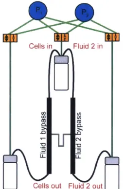
1.2.2.2 Measuring density with a dual cantilever

The dual cantilever method was initially described in Bryan, 2011, and in greater

detail in Bryan et al, 2014 (33, 38) as an alternative to the single SMR that allows for

*~

~

multiple density measurements to be made simultaneously. Placing two cantilevers in

series eliminates the requirement for the waiting period to measure the buoyant mass of a

cell in Fluid 2. To measure the buoyant mass of single cells in two different density fluids

in a continuous flow format, devices with two fluidically connected and simultaneously

operated SMRs were fabricated and tested (Figure 1.2-6). During operation of the dual

SMR, a dilute cell population suspended in cell media (Fluid 1), is delivered to the sample

bypass via pressure-driven flow (Figure 1.2-6 and Figure 1.2-7), and single cells flow into

the first SMR (SMR1) for the first buoyant mass measurement. The cells then travel

through a microchannel to a cross-junction, where a high density fluid is introduced. After

the cross-junction, cells continue through a long serpentine channel, which facilitates

mixing of the two fluids. The cells next enter a second cantilever (SMR2) for a buoyant

mass measurement in the mixed fluid (Fluid 2). As cells flow through each cantilever, a

change in resonance frequency is recorded, which is determined by each cell's buoyant mass

04

fn

n

ld

High density fluid bypass

I Figure 1.2-6. Schematic of the dual SMR measurement.

A single cell flows from the sample bypass channel into the first SMR (SMR1) for a buoyant

mass measurement in Fluid 1 (red), typically cell media. The cell then continues to a cross-junction where a high density fluid (blue) is introduced and mixes with Fluid 1 via

diffusion in the serpentine channel. The second buoyant mass measurement is recorded as the particle flows through the second SMR (SMR₂) in this mixed fluid (Fluid 2, lavender). Relative values for applied pressure are indicated with green (high), orange (mid), and gray (low) circles, and the closed circle on the waste bypass denotes the location of a plug.

Cells out 9Kaqe flow

L.L

High density fluid

WP Waste

Figure 1.2-7. Diagram of fluidic and pressure components in the dual SMR.

Solenoid valves (orange rectangles) set waste vial pressures to those of the pressure

regulators (blue circles) or to atmosphere. A plug (circled black X) forces waste fluid into a single vial. Black lines indicate fluidic tubing, and green lines indicate pneumatic tubing.

Although the dual SMR design is amenable to increased throughput, several

non-obvious challenges to precision measurements in a low Reynold's number (Re~0.8)

environment were evident during testing of preliminary designs. Three critical design

features address these challenges and facilitate the measurement: (1) differently-sized

cantilevers to prevent signal cross-talk; (2) a microfluidic cross-junction to steadily

introduce a second fluid; and (3) a narrow serpentine channel to facilitate mixing the two

fluids.

The first design feature, differently-sized cantilevers, minimizes crosstalk of the

signals measured from SMR1 and SMR2. Crosstalk results from mechanical coupling

between the vibrations of similarly sized cantilevers with their out-of-phase neighbors. If

the two cantilevers in the dual SMR have similar dimensions, their resonance frequencies

are similar; thus, the mechanical vibrations of one will apply an auxiliary driving force on

its neighbor. Significantly altering the geometry of one cantilever (300 and 360pm length

for SMR1 and SMR2, respectively) eliminates crosstalk by ensuring that the two resonance

frequencies are different.

The dual SMR's second critical design feature is a microfluidic cross-junction that

consistently introduces a second fluid of higher density. The addition of this high density

fluid may occur by either a cross-junction or a T-junction (Figure 1.2-8). The time required

for two fluids to mix across a channel is approximately four times smaller in a

cross-junction design relative to a T-cross-junction because mixing occurs at two interfaces rather than

just one. What is not readily apparent is how differently the two configurations perform in

the presence of cells. Variations in pressure occur as large-sized cells pass the microfluidic

junctions and enter the high resistance serpentine channel. These pressure changes alter

the relative amount of high density fluid introduced at the junction and create changes to

fluid density along the serpentine channel, which adversely affect the SMR2 baseline

stability at the time of the large cell's measurement. However, baseline stability for cells

already in the vicinity of SMR2 is not adversely affected. The cross-junction design better

dampens these effects due to its larger interface between the two fluid streams, as

compared to the T-junction design (Figure 1.2-8). We selected the cross-junction design for

all cell measurements. In this design, SMR2 baseline changes in the vicinity of a cell

measurement are typically ~1 x 10-5 g/mL, a value which corresponds to a <0.01% change

Narrow T-junction Wide T-junction Cross-junction

01

YIJIIUMIIbT

(~)

0

T~1J{fLLtJTJT

'It-

r

Figure 1.2-8. Comparison of different dual SMR channel designs.

The designs evaluated include the narrow T-junction (A), wide T-junction (B), and cross-junction (C). Schematics of the channel configurations are shown in the top row of the figure. Fifty seconds of acquired frequency data from SMR2 are shown in the middle section. Insets are of peaks highlighted by red boxes in each frequency trace. The uniform peak shape and low baseline variation in the cross-junction design demonstrate its

superiority over the narrow T-junction and wide T-junction.

To ensure that each cell is immersed in a near-homogeneous solution when

measured in SMR2, the dual SMR has a 5000 pim long serpentine channel, and flow rates

are set such that the lag time for cells traveling from SMR1 to SMR2 is greater than ten

seconds. In a 25 ptm wide serpentine channel, the time required for the fluid mixture to

reach 95% homogeneity is approximately six seconds, and in principle, the dual SMR

enables cell mass, volume, and density measurements at a faster rate than the single SMR, A

60, 200

approximately two cells per second. Increased flow rate, higher data acquisition rate, a

longer serpentine channel, and lower viscosity fluids would improve throughput without

sacrifice to measurement resolution. Cell rupture and other negative effects on cell

viability are not expected to occur at increased flow rate. In the same way that junction

design affects baseline stability, serpentine channel geometry is also important; a wider

serpentine channel introduces even greater baseline instability than a narrow channel. In

the wide T-junction design (Figure 1.2-8), the baseline frequency instabilities are more than

10 times those observed in other designs. Thus, pressure damping features (Figure 1.2-8)

at the point of fluid introduction and high downstream channel resistances are critical to

achieving a stable system when particles are sized close to that of the channel. These

features are included in the cross-junction design.

1.2.2.3 Comparison of the two methods

There are several challenges associated with operating the dual SMR, most of which

relate to its sensitivity to changes in pressure and high channel resistances. The pressures

at the start of an experiment must be carefully balanced to ensure proper direction and

speed of fluid flow at all inlets and to maintain the desired composition of Fluid 2. During

the course of the experiment, the fluid height in each of the vials gradually changes, and so

the pressures must be monitored and adjusted periodically. Pressure adjustments are

implemented by either changing the setting on an electronically controlled pressure

regulator (resolution = 0.006 PSI) or by manually adjusting the vertical height of the fluid

vials. These methods allow changes to fluid flow rates by -0.02%. Large-sized cells

introduce baseline instabilities, and bubbles and small pieces of debris also upset the

pressure balance. Filtering all fluids and a lengthy flushing procedure (five to seven

occasionally disrupts the system. Because the channel volume of the dual SMR is so much greater than that of the single SMR, the likelihood of trapping debris or generating bubbles is much greater; similarly, isolating the source or location of each of these issues is more challenging in the dual SMR.

One practical consideration when operating the dual SMR relates to selecting a cell concentration that allows for a reasonably steady baseline. When a cell passes through the cross-junction into the serpentine channel, it causes a local fluctuation in the composition of

Fluid 2. Thus, when many cells are measured in quick succession, the baseline becomes less steady, which increases the uncertainty in determining the fluid density. One

approach to solving this problem is to increase the fraction of high density fluid delivered to the serpentine channel. This requires the high density fluid to be delivered with higher pressure, which makes pressure fluctuations from cells less significant. So as not to

sacrifice measurement accuracy, the increased pressure also requires adjustments to slow

the pQaQ g of eal1, wQbich l1

OWs flijvl flow in tie Qytem overnll and ruii1t. in an over.all

steadier baseline. These adjustments, however, reduce the rate at which cells can be measured. Although in principle the dual SMR should be able to measure approximately two cells per second, the most reliable operation is achieved when cells enter SMRi at approximately one cell every ten seconds, which is comparable in throughput to the fluid-switching method for measuring density presented by Grover, et al (32). Thus, practical considerations associated with the existing design currently limit its overall performance.

The primary throughput limitation of the single cantilever, however, relates to its inability to measure cells serially. Thus, once a single cell enters the cantilever, no additional cell can be measured until the original cell is returned from the Fluid 2 bypass channel. During this process, a significant volume of cells is flushed by the Fluid 1 bypass

channel, resulting in some loss of sample, and limiting the usefulness of the technique in

measuring rare cells. Nonetheless, refinements in the measurement technique have

resulted in a throughput that exceeds that reported in Grover et al, 2011. Additionally, this

method suffers far less from the baseline instabilities associated with the dual SMR, has

fewer narrow channels and is thus less susceptible to clogging, and involves balancing the

pressure among four, rather than six ports, ensuring a simpler and more reproducible

measurement.

1.2.3 Approaches for minimizing measurement error

1.2.3.1 Effect of Fluid 2 density on density measurement error

Density variation measured in a cell population can result from natural biological

heterogeneity and error in the measurement technique. One source of error in the

measurement technique arises from the value of the density of Fluid 2 relative to the

density of the measured cells. Though Fluid 1 is almost always cell media, the composition

of Fluid 2 can be adjusted by adjusting the vial heights and peak wait times in the single

cantilever method, or the pressure ratio between the channels meeting at the cross-junction

in the dual cantilever method. The effect of the Fluid 2 density value on measurement

error was estimated by applying multiplicative and additive errors to average L1210 cell

buoyant masses in Fluid 1 and a range of Fluid 2 values, measured in the dual SMR.

Multiplicative error results from an uncertainty in determining the cell's exact

lateral position in the tip of the cantilever channel (39). This error, estimated from the

buoyant mass distribution of polystyrene beads (Figure 1.2-14), is inversely dependent on

particle radius and directly proportional to buoyant mass. Thus, minimizing this error

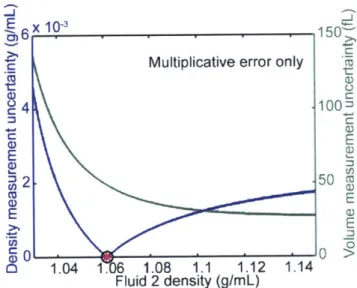
mass. In the theoretical case of pure multiplicative error, uncertainty in determining the

density of the cell will be at a minimum when the density of Fluid 2 matches that of the cell

(Figure 1.2-9). Here the cell buoyant mass is zero, as is the associated error, and measuring

Fluid 2 density is sufficient to determine the density of the cell. As the density of Fluid 2

deviates from that of the cell, the magnitude of the cell's buoyant mass in Fluid 2 will

increase, as will the associated density measurement error. Interestingly, multiplicative

error in the volume measurement continually decreases for higher Fluid 2 densities (Figure

1.2-9). This decrease is graphically indicated as a decreasing standard error in the slope

(Figure 1.2-1) where the x-axis (fluid density) distance increases between the two buoyant

mass measurements.

Multiplicative error only

4 100 2. 5 E o 50-a-_E O 1.04 1.06 1.08 1.1 1.12 1.14 Fluid 2 density (g/mL)

Figure 1.2-9. Measurement uncertainty as a function of Fluid 2 density in the case of

purely multiplicative error.

The uncertainty of cell density is shown in blue, and the uncertainty of cell volume is

shown in green. The actual cell density is indicated by a pink asterisk. The minimum uncertainty in the density measurement is indicated with a black circle. The uncertainty in volume decreases continuously with increasing Fluid 2 density.

A second form of error is additive error, which results from a constant baseline noise

and leads to uncertainty in determining peak height and thus cell buoyant mass (40). In

density occurs when the density of Fluid 2 is greater than the density of the cell (Figure 1.2-10). Under the conditions of our simulation, the minimum value occurs when the fluid density is approximately 1.15 g/mL. Beyond this minimum, the uncertainty increases at a relatively slow rate. Similarly to the case of multiplicative error, uncertainty in the volume measurement due to additive error decreases as the difference between Fluid 1 and Fluid 2 increases (Figure 1.2-10).

X~ 10-1

-E3 6

Additive error only

02 .40 a)

E

E

o

Figure 1.2-10. Measurement uncertainty of cell density or cell volume is a function of Fluid 2 density in the case of purely additive error.

The uncertainty of cell density is shown in blue, and the uncertainty of cell volume is shown in green. The actual cell density is indicated by a pink asterisk. The minimum uncertainty in the density measurement is not shown, and the uncertainty in volume decreases continuously with increasing Fluid 2 density.

When multiplicative and additive errors are both present, as is the case with the dual SMR, each dominates different measurement regimes. Multiplicative error dominates when buoyant mass is relatively large and additive error dominates when buoyant mass is relatively small. When both forms of error are present, the error in the cell density

measurement is minimized where the Fluid 2 density is slightly greater than cell density (Figure 1.2-11). Here multiplicative error is small and additive error dominates, meaning density measurement error is mainly determined by noise in the instrument baseline.

When Fluid 2 density deviates from this minimum, multiplicative error dominates, and

density measurement error increases. Volume measurement error decreases

asymptotically as the difference between Fluid 1 and Fluid 2 increases. Thus, to optimize

the measurement error for both density and volume, the Fluid 2 density should be

somewhat greater than that of the cell.

E8 10~ . 200 zz c,4 100 CE 250 E E C, 1.04 1.06 1.08 1.1 1.12 1.14 Fluid 2 density (g/mL)

Figure 1.2-11. Measurement uncertainty of cell density and cell volume as a function of Fluid 2 density, assuming no uncertainty in measuring fluid density.

The uncertainty of cell density is shown in blue, and the uncertainty of cell volume is shown in green. The simulation is calculated using fixed values for buoyant mass in Fluid

1, L1210 cell density, and Fluid 1 density, along with a range of experimentally relevant

values for Fluid 2 density, which correspond to a range of buoyant masses in Fluid 2. Multiplicative error is applied to the simulated measurements based on the variation in buoyant masses of polystyrene beads, and additive error is applied using the magnitude of the baseline noise in each cantilever. The Fluid 2 density of a typical experiment in the dual SMR is adjusted to approximately 1.07 g/mL 1. The pink asterisk indicates the cell density, and the black circle corresponds to the point of minimum uncertainty in the density measurement. Uncertainty in volume decreases continuously with increasing Fluid 2 density.

The effect of the value for Fluid 2 density is especially pronounced when performing

the dry density measurement discussed in 1.2.1.1. As discussed in the above section,

minimizing measurement error requires that the Fluid 2 density be somewhat greater than that of the cell. However, the dry density of the cell is close to 1.4 g/mL, and the density of D20-PBS is approximately 1.1 g/mL. Thus, in this case, the Fluid 2 density is significantly

lower than that of the cell. To determine the effect of this difference on measurement error, a simulation was performed by calculating the cell density from a population of buoyant masses with a range of uncertainties comparable to the noise of the SMR used in

conducting the measurements shown in this manuscript (0.05 - 1 Hz). The same level of

uncertainty was added to both the buoyant mass in Fluid 1 and in Fluid 2. Only additive error was considered in this case. As shown in Figure 1.2-12, the effect of additive error on the density measurement (A, B) is much less pronounced than on the dry density

measurement (C, D).

An important metric when considering this error is how the variance of the

simulated population compares with that of an experimentally measured population. If the width of the simulated distribution is smaller than that of the experimental population, then the distribution of the population can be estimated to be dominated by biological variability rather than measurement error. To make this estimation, the experimental population was compared to the simulated distribution corresponding to 0.5 Hz

measurement noise, as this was a value most closely representing the instrument noise during a typical experiment. As shown in Figure 1.2-12B, the width of the simulated population of the density measurement is much smaller than the experimental population; however, the width of the simulated dry density measurement distribution is fairly close to

that of the experimental population (Figure 1.2-12D), suggesting that the true, biological variability in this parameter may be smaller than that obtained under the measurement conditions shown here. Because the maximum value for the Fluid 2 density is capped at the value for D20 (-1. 1 g/mL), other approaches to minimize error in the dry density measurement, likely involving improvements to the optical and electronic components of the system, must be utilized.

B

A

C

IH

---

1 11

f-n

Figure 1.2-12. Comparing the effects of additive error when measuring total density and dry density.

Scatter plots (A and C) represent the effect of additive error applied to peak height

measurements in Fluid 1 and Fluid 2 at values indicated in legend (0.05 - 1 Hz). Bar graphs (B and D) represent overlay of simulated density distribution with additive error of

0.5 Hz (red curve) over distribution of experimental data (gray bars).

1.2.3.2 Second mode actuation to reduce measurement error

Another means of reducing the error in the density measurement is to actuate the

SMR in second mode (Figure 1.2-13) (28, 39). This type of actuation, typically requiring a

higher amplitude driving force, is characterized by the introduction of a node midway along

the cantilever, or a region that remains stationary while other regions in the cantilever are

in motion. Thus, while a cantilever resonating in first mode has only one region of high

46

I

~

D

amplitude motion, and therefore high sensitivity, at the peak, a cantilever resonating in

second mode has an additional region of high sensitivity at the antinode, situated between

the fixed cantilever base and the node (Figure 1.2-13B, blue arrow). The multiplicative

error discussed in 1.2.3.1 results from variation in the exact lateral position of a particle at

the cantilever tip; a particle traveling on the outer wall of the fluidic channel of the

cantilever will lead to a greater frequency shift than an identical particle traveling along

the inner wall. However, frequency shifts measured at the antinodes are insensitive to the

position of the particle in the fluidic channel, and are therefore free of multiplicative error

(39). Thus, for data obtained with a second mode measurement, the antinode peaks are

averaged to determine the buoyant mass, and the value of the middle peak is disregarded.

Peak in Fluid 1 Peak in Fluid 2

A

" C: > L)

C

C. C

Cantilever _{Time (s) Time (s)} x-position

B

Cr N

L.L U.

Cantilever Time (s) Time (s)

x-position

Figure 1.2-13. Cantilever mode shape and peak shape in first and second modes.

First mode actuation is shown in the first row (A), and second mode actuation is shown in the second row (B). Double-headed arrows in the first column indicate the motion of the cantilever tip (red) or antinode (blue, bottom). The green arrow in the first column of (B) indicates the position of the node. Single-headed arrows in the middle and right-hand columns indicate peak locations corresponding to cantilever positions indicated by the arrows of matching color in the first column.