Publisher’s version / Version de l'éditeur:
The Journal of Physical Chemistry A, 118, 51, pp. 12069-12079, 2014-10-14
READ THESE TERMS AND CONDITIONS CAREFULLY BEFORE USING THIS WEBSITE.
https://nrc-publications.canada.ca/eng/copyright
Vous avez des questions? Nous pouvons vous aider. Pour communiquer directement avec un auteur, consultez la
première page de la revue dans laquelle son article a été publié afin de trouver ses coordonnées. Si vous n’arrivez pas à les repérer, communiquez avec nous à [email protected].
Questions? Contact the NRC Publications Archive team at
[email protected]. If you wish to email the authors directly, please see the first page of the publication for their contact information.
NRC Publications Archive
Archives des publications du CNRC
This publication could be one of several versions: author’s original, accepted manuscript or the publisher’s version. / La version de cette publication peut être l’une des suivantes : la version prépublication de l’auteur, la version acceptée du manuscrit ou la version de l’éditeur.
Access and use of this website and the material on it are subject to the Terms and Conditions set forth at
Short-time dynamics at a conical intersection in high-harmonic
spectroscopy
Patchkovskii, Serguei; Schuurman, Michael S.
https://publications-cnrc.canada.ca/fra/droits
L’accès à ce site Web et l’utilisation de son contenu sont assujettis aux conditions présentées dans le site LISEZ CES CONDITIONS ATTENTIVEMENT AVANT D’UTILISER CE SITE WEB.
NRC Publications Record / Notice d'Archives des publications de CNRC:
https://nrc-publications.canada.ca/eng/view/object/?id=aad3fd82-4d1b-46b5-8a04-31cbd7427a52 https://publications-cnrc.canada.ca/fra/voir/objet/?id=aad3fd82-4d1b-46b5-8a04-31cbd7427a52
Short-Time Dynamics at a Conical Intersection in High-Harmonic
Spectroscopy
Serguei Patchkovskii*
,†and Michael S. Schuurman
‡,¶ †Max Born Institute, Max-Born-Straße 2A, 12489 Berlin, Germany
‡
Steacie Laboratories, National Research Council of Canada, 100 Sussex Drive, Ottawa, Ontario K1A 0R6, Canada
¶
Department of Chemistry, University of Ottawa, 10 Marie Curie, Ottawa, Ontario K1N 6N5, Canada
ABSTRACT: High-harmonic spectroscopy probes molecular dynamics using electrons liberated from the same molecule earlier in the laser cycle. It affords sub-Ångstrom spatial and subfemtosecond temporal resolution. Nuclear dynamics in the intermediate cation influence the spectrum of the emitted high-harmonic photons through an autocorrelation function. Here, we develop an analytical approach for computing short-time nuclear autocorrelation functions in the vicinity of conical intersections, including laser-induced and nonadiabatic coupling between the surfaces. We apply the technique to two molecules of current experimental interest, C6H6and C6H5F. In both molecules, high-harmonics generated within the same electronic channel are not sensitive to
nonadiabatic dynamics, even in the presence of substantial population transfer. Calculated autocorrelation functions exhibit significant deviations from the expected Gaussian decay and may undergo revivals at short (∼1.5 fs) times. The associated phase of the nuclear wavepacket provides a possible experimental signature.
■
INTRODUCTIONAtoms and molecules subjected to intense (I ≈ 1014W cm−2) infrared (IR) laser fields emit high-harmonics of the driving light,1 extending into the extreme ultraviolet and soft X-ray energy range.2The high-harmonic generation (HHG) process
can be qualitatively understood within the three-step model3,4 (see also refs 5 and 6 for recent reviews). HHG is initiated when an electron is liberated from a molecule near the peak of the electric field of the laser cycle. The electron is then accelerated by the laser field and can be driven back to the ion core with energies up to 3.2 × Up, where Up is the ponderomotive energy (e.g., Up ≈ 6.0 eV for I = 1014 W cm−2and λ = 800 nm). Recombination of the electron, which occurs within the same laser cycle up to a few femtoseconds after the ionization event, can then lead to emission of an energetic photon.
In typical experimental conditions, the HHG photon energy uniquely determines both the ionization and recombination time.4,7This mapping creates a clock, which enables imaging of the short-time dynamics in an atom or molecule with ∼100 as time and sub-Ångstrom spatial resolution.5,6 Furthermore, because the probing electron is coherent with the ion core, the phase of the ion’s wave function is mapped onto the phase of the harmonic radiation. The harmonic phase is exper-imentally accessible and can be used to disentangle different contributions to the HHG spectra.8−11 The unprecedented
time and spatial resolution of the HHG probe have been used to image electronic wave functions,12 observe real-time dynamics of electronic13 and nuclear14 wavepackets, pinpoint
the exact time of the ionization event,15 and probe electron
correlation.16,17 Possibilities for extending HHG spectroscopy into the solid-state domain have been discussed as well.18
Despite the fleeting existence of the intermediate cation in the three-step HHG process, emitted radiation is affected by the nuclear motion on the cationic potential energy surface (PES) between the moments of ionization tiand recombination
tr. These nuclear dynamics induce substantial isotope effects in high-harmonic emission from molecules.19−22 Quantum-path interference can be used to observe coherent nuclear motion in the intermediate cations even in the absence of isotopic substitution.23
To a first approximation, the harmonic intensity is proportional to the square modulus of the nuclear autocorre-lation function η24
η( )t = ⟨Ψnuc( )ti |Ψnuc r( )t ⟩ (1)
Other effects arise in long driving pulses;25 these more conventional terms are related to the field-induced dynamics of the parent molecule rather than the intermediate cation. Here, we assume that the driving pulse is sufficiently short not to perturb the system prior to the ionization event.
The phase of the autocorrelation function enters the overall HHG emission phase.24 For cations well-described by an isolated electronic energy surface, |η|2 is typically a Gaussian function of time,26while its phase arg(η) grows linearly with
Special Issue: David R. Yarkony Festschrift
Received: September 7, 2014
Revised: October 14, 2014
Published: October 14, 2014
time.9 Parameters of short-time autocorrelation functions for isolated electronic states are routinely available in most species of chemical interest.26−29
At the same time, in many molecular cases, the intermediate cation is formed either directly on top of a conical intersection (CI) (e.g., CH4, C6H6) or in the immediate vicinity of a CI (e.g., CF3H and most substituted methanes; C6H5CH3 and most substituted benzenes; etc.). While nuclear dynamics at a CI are known to be rich and complex on vibrational and chemical time scales,30 it can also be expected to lead to
nontrivial effects in HHG spectroscopy. The twin goal of this work is to develop a simple, computationally tractable model of short-time coherent nuclear dynamics on multiple, coupled electronic surfaces and to explore some of its consequences for the nuclear autocorrelation functions and HHG.
■
THEORYHHG experiments are usually performed on cold, rigid target molecules in a vibrational ground state. Upon ionization, the compact ground-state vibrational wave function is projected onto the cationic energy surface(s). Due to the small spatial extent of this initial wavepacket and the short temporal evolution, it appears sufficient to the approximate cationic energy surface(s) by a quadratic expansion in the vicinity of the initial neutral geometry.
The analytical theory of short-time nuclear autocorrelation functions on a single, quadratic PES has been given previously.26 In ref 26, nuclear wave functions of the intermediate cation are expanded in terms of harmonic oscillator functions of the neutral PES. The difference between the cationic and the neutral PES is then treated as a perturbation to the (trivially known) dynamics of the multidimensional harmonic oscillator solutions. This expansion provides a compact, convenient representation of the evolving vibrational wavepacket at short times. It additionally side steps the issue of unbound electronic states in the cation. We choose the same basis for the nuclear degrees of freedom in the present multisurface treatment.
A multisurface treatment of nuclear dynamics in HHG spectra of SF6 was given previously.31,32 However, this treatment focuses on impulsive Raman processes before the ionization event and neglects coupling between electronic surfaces between the moments of ionization and recollision. As will be seen below, neglect of electronic surface coupling may be unjustified in the more general case.
In the following, we denote vector quantities using bold letters. Individual elements are indicated by subscripts, with the quantity given in the regular typeface. For example, niis the ith element of vector n. Unless noted otherwise, all quantities and expressions are given in atomic units (|e| = me= ℏ = 1).
Time Series Expression for the Nuclear Autocorrela-tion FuncAutocorrela-tion.We expand the vibronic wave function of the cation as a linear combination of direct products between electronic |Ψi⟩and nuclear |n⟩ wave functions
∑
|r q, ,t⟩ = a ( )et − ϵ ℏ|Ψ( ; )r q ⟩| ⟩n i i t i n n in/ (2)Clamped-nuclei electronic wave functions |Ψi(r;q)⟩ are assumed to be orthonormal in the space of electronic coordinates r
δ
⟨Ψi( ; ) ( ; )r q |Ψjr q ⟩ = ij (3)
Electronic wave functions depend parametrically on nuclear coordinates q. However, we do not at this point assume a particular relationship between the electronic Hamiltonian Ĥel and wave functions Ψi.
Nuclear basis functions |n⟩ are chosen as eigenfunctions of a multidimensional harmonic potential ν0 with nuclear kinetic energy operator T̂N
ν
̂ + | ⟩ = ϵ | ⟩
T q n n
( N 0( )) n (4)
Harmonic potential ν0 is, in principle, arbitrary and can be chosen for convenience; in our case, the most appropriate choice is the harmonic expansion of the neutral PES in the vicinity of the equilibrium geometry.
The number of quanta in the ith mode of eigenfunction |n⟩ is given by ni ≥ 0. The energy of basis function |n⟩ is ϵn= ∑i ℏωi(ni+ (1/2)), with ωibeing the characteristic frequency of the ith mode. Finally, the explicit form of |n⟩ is
∏
πω ω | ⟩ = ℏ ! ℏ ω − − ℏ ⎜ ⎟ ⎜ ⎟ ⎛ ⎝ ⎞ ⎠ ⎛ ⎝ ⎜⎜⎛⎝ ⎞⎠ ⎞ ⎠ ⎟⎟ n H q n (2 ) e i i n i q n i i 1/4 1/2 ( /2 ) 1/2 i i i i 2 (5)where normal coordinates q are linear combinations of Cartesian displacements r
∑
= qi Q m r a ai a1/2a (6)with Qaibeing the eigenvectors of the mass-weighted Hessian
ν = ∂ ∂ ∂ − − H m m r r ab a b a b 1/2 1/2 2 0 (7)
By construction, q = 0 at the neutral equilibrium geometry. Inserting the ansatz of eq 2 into the time-dependent Schrödinger equation for the Hamiltonian T̂N+ Ĥel + Ĥl and projecting the result onto ⟨m|⟨Ψj|eiϵmt/ℏ, we obtain the expected result for the time derivatives of the expansion coefficients ȧj,m
∑
ν ν δ ν ℏ ̇a = ϵ −ϵ ℏ⟨ | −m + + ̂g +g | ⟩n i j e i t ji ji ji ji ji m n , i(m n) / e 0e l (1) (2) (8)Operators νjie and νjil are, respectively, matrix elements of the field-free electronic Hamiltonian Ĥeland the (time-dependent) laser interaction Hamiltonian Ĥl. The first- and second-order nonadiabatic coupling operators33 are given, respectively, by
ĝji(1)and gji(2) νjie= ⟨Ψ| ̂ |Ψ⟩jHel i (9) νjil = ⟨Ψ| ̂ |Ψ⟩jHl i (10)
∑
̂ = −ℏ ⟨Ψ| ∂ ∂ |Ψ⟩ ∂ ∂ g M q q ji s s j s i s (1) 2 (11)∑
= − ℏ ⟨Ψ| ∂ ∂ |Ψ⟩ g M q 2 ji s s j s i (2) 2 2 2 (12)where Ms is the effective nuclear mass corresponding to coordinate qs.
Explicit expressions for matrix elements of the multiplicative potential ⟨m|νjie − ν0δji|n⟩ have been given previously26 and need not be restated. Evaluation of matrix elements ⟨m|ĝji(1)|n⟩ is tedious but, in principle, straightforward and is discussed in
the following section. In keeping with the common practice,34 we choose to neglect matrix elements of gji(2). For the purpose of computing wavepacket dynamics, it is convenient to combine matrix elements of all time-independent operators in eq 8
ν ν δ
= ⟨ | − + ̂ + | ⟩
Cj im n m jie 0 ji gji(1) gji(2)n (13)
For the long-wavelength IR driving laser fields, it is appropriate to consider the matrix elements of νjil within the dipole approximation. Furthermore, because subcycle dynamics are of primary interest, it is sufficient to take the laser field within the continuous-wave (CW) approximation and disregard the envelope. In the length gauge, the resulting matrix elements are given by ν ⟨ | | ⟩ =m jiln Dj im ncos(Ω + Φt ) (14) = −⟨ | · | ⟩ Dj im n m F d nji (15)
∑
= −⟨Ψ| r|Ψ⟩ dji j a a i (16)where Ω is the frequency of the laser field, Φ is the field phase at the time when the wavepacket is created, and F is the amplitude of the laser electric field. Permanent dipoles dii describe the linear Stark shift of the electronic surfaces, while the transition dipoles dij(j ≠ i) are responsible for the field-induced population transfer between the surfaces.35
While it is possible to propagate eq 8 numerically, at short times, it seems natural to develop an analytical expression for the amplitudes ain by expanding them in a power series of time26
∑
= ! = a t s A t ( ) 1 i s i s s n n 0 ( ) (17)Substituting eq 17 into eq 8, we obtain
∑
∑
∑
∑
∑
ℏ ! = + ! ! × ϵ − ϵ !ℏ = + = = = ⎛ ⎝ ⎜⎜ ⎞ ⎠ ⎟⎟ A t s C D t r f A t s t p i i ( ) s js s i j i j i r r r s is s p p p p p m n m n m n n m n 0 ( 1) 0 ( ) 0 ( ) 0 (18)where the time-dependent interaction with the laser field has also been expanded in power series with coefficients
= Ω + Φ |= f t t d d cos( ) r r r t ( ) 0 (19)
Collecting terms in the same order of t in eq 18, we immediately obtain
∑
∑
= − ℏ ! ! − ! ϵ − ϵ ℏ + ϵ − ϵ ℏ ! − ! ! + − − ⎡ ⎣ ⎢ ⎢ ⎛ ⎝ ⎜ ⎞ ⎠ ⎟ ⎛ ⎝ ⎜ ⎞ ⎠ ⎟ ⎤ ⎦ ⎥ ⎥ A A l p l p C D p p r r f i ( ) i( ) i( ) ( ) j l i p i l p j i p j i r p r r m n n m n m n m n m n ( 1) ( ) ( ) (20)For the CW laser field, it is possible to further simplify the second term in the square bracket in eq 20. Indeed
∑
∑
ϵ − ϵ ℏ ! − ! ! = ϵ − ϵ ℏ ! − ! ! Ω = ϵ − ϵ ℏ + Ω + ϵ − ϵ ℏ − Ω − − Ω +Φ Ω +Φ − Ω +Φ ⎜ ⎟ ⎜ ⎟ ⎛ ⎝ ⎜ ⎞ ⎠ ⎟ ⎛ ⎝ ⎜ ⎞ ⎠ ⎟ ⎛ ⎝ ⎞ ⎠ ⎛ ⎝ ⎞ ⎠ p p r r f p p r r i( ) ( ) i( ) ( ) [(i ) e ] 1 2e i 1 2e i r p r r r p r r t t p p t p p m n m n m n m n ( ) i( ) i( ) i( ) 9 (21)Substituting eq 21 into eq 20, we therefore obtain
∑
= − ℏ ! ! − ! ϵ − ϵ ℏ + ϵ − ϵ ℏ + Ω + ϵ − ϵ ℏ − Ω + − Ω +Φ − Ω +Φ ⎜ ⎟ ⎜ ⎟ ⎡ ⎣ ⎢ ⎛ ⎝ ⎜ ⎞ ⎠ ⎟ ⎧ ⎨ ⎩ ⎛ ⎝ ⎞ ⎠ ⎛ ⎝ ⎞ ⎠ ⎫ ⎬ ⎭ ⎤ ⎦ ⎥ A A l p l p C D i ( ) i( ) 1 2 e i e i jl i p il p j i p j i t p p t p p m n n m n m n m n m n m n ( 1) ( ) i( ) i( ) (22)This is our final working expression, providing a generalization of the result of ref26to the case of multiple, coupled electronic surfaces in the presence of an intense IR field.
Choice of the Electronic Wave Function Ansatz.Up to now, we refrained from specifying electronic wave functions Ψi(r;q). Equation 22 is valid for any orthonormal set of electronic wave functions, including those that define either adiabatic or diabatic states. In terms of computational simplicity, a particularly appealing choice is the so-called crude adiabatic ansatz,36where the electronic wave functions are assumed to be independent of the nuclear coordinates
Ψi( ; )r q ≈ Ψi( ;r q0) (23)
For electronic wave functions satisfying eq 23, all nonadiabatic terms (both first- and second-order, eqs 11 and 12) vanish identically. Matrix elements of eq 9 reduce to Hellmann− Feynman forces on the nuclei,37 while the coordinate dependence of the permanent and transition dipoles in eq 16 vanishes.
The accuracy of the crude adiabatic ansatz depends critically on the number of electronic states considered in the expansion. The simplest form of the crude adiabatic approximation used presently includes only the electronic states essential at the expansion point by itself. Such a limited expansion is known to be wildly inaccurate for long-time dynamics.38,39We therefore also consider the standard adiabatic ansatz, where electronic wave functions are taken to be eigenfunctions of the clamped-nuclei electronic Hamiltonian. In this case, the potential νjie becomes diagonal in i,j
νjie=ν δii ije (24)
and can be expanded to any desired order in q. At the same time, the gradient-coupling operator (eq 11) must be evaluated. This operator becomes singular at the CI seam,40 requiring
special care in evaluation of the corresponding matrix elements (see below).
Compact Analytical Representation for the Short-Time Autocorrelation Function.Although eq 17 in principle contains all of the information on the wavepacket evolution, including the norm and the phase of the autocorrelation
function, its practical applications may require rather high-order coefficients Ain(s) (up to order 120 in some of the examples discussed below). In many cases, knowledge of the overall shape of |η|2(eq 1) is sufficient. It is therefore both useful and instructive to develop a more compact, approximate form for the autocorrelation function norm.
The time-dependent Schrödinger equation for the wave-packet amplitudes (eq 8) is in the general form
∑
̇ = ϵ + a a b a i k k k l kl l (25)Assuming that all coefficients ϵkand bklcan be chosen as real, the rate of change of population of a basis function k, ck= |ak|2, is therefore given by
∑
̇ = ̇ =† − ≠ † † ⎛ ⎝ ⎜⎜ ⎞ ⎠ ⎟⎟ c a a c b a a a a ( ) i k k k k l k kl l k l k (26)In the common case of the initial wavepacket being a replica of the ground-state vibrational eigenfunction of the neutral species, |η(t)|2= c
0(t).
In the weak coupling limit, we can assume that ak ≈ (ck)1/2e−iϵkt−iϕk, so that
∑
̇ ≈ − ̃ ϵ − ϵ ≠ ⎛ ⎝ ⎜ ⎞ ⎠ ⎟ c c b c c t 2 sin(( ) ) k k l k kl l k l k 1/2 (27)where the phase of coefficient ak has been absorbed into the definition of bkl, yielding b̃kl. Furthermore, weak coupling implies that the steady-state approximation is applicable at almost all times, so that (cl/ck) ≈ const and
∑
α ̇ ≈ − ≠ c 2c f sin( )t l l l 0 0 0 (28)Equation 28 is readily integrated, giving the desired analytical form of the autocorrelation function
∏
α = − c t( ) exp( (1g cos( )))t l l l 0 (29)If one of the αl coefficients (e.g., α1) is small, g1(1 − cos(α1t)) ≈ (g1α12/2)t2, and the corresponding term in eq 29 becomes a Gaussian.26 The physical origin of this Gaussian
decay term can be qualitatively understood by considering an initially stationary particle, placed on a surface of a constant slope. Under the action of a constant force, the momentum
P(t) of the particle will increase linearly with time, while the
displacement R(t) will grow quadratically. Semiclassically, the test particle corresponds to a one-dimensional Gaussian wavepacket of constant width w
ψ π = ⎜⎛ ⎟ − − − − ⎝ ⎞ ⎠ x t w ( , ) 2 e e t w x R t P t x R t 1/4 ( ( ))2 i ( )( ( ))
The corresponding autocorrelation function is given simply by
∫
ψ ψ= | † | = − −
I tt( ) t( , ) ( , 0) dx t t x x2 e P t( ) /(4 )2 we wR t( )2
At short times, this expression is dominated by the change in the central momentum of the wavepacket, yielding a Gaussian function of time. At somewhat longer times, calculated autocorrelation functions start to deviate from the pure Gaussian form.26 Retaining one correction term in eq 29 in addition to the leading Gaussian, we then obtain a
three-parameter phenomenological expression for the square modulus of the autocorrelation function
γ α
= −β −
c t0( ) e t2exp( (1 cos( )))t (30)
Coefficients α, β, and γ can be obtained by matching derivatives of eq 30 to low-order coefficients Aj(k) from eq 22. Adding further correction terms to eq 30 yields no improvement in the fit at short times and was not pursued further. Below, we compare fits from eq 30 to the calculated autocorrelation function norms.
■
COMPUTATIONAL DETAILSWe consider two examples for short-time dynamics in the vicinity of a CI, benzene C6H6and fluorobenzene C6H5F. In benzene, the initial wavepacket is created directly on top of the CI seam. In fluorobenzene, the two surfaces are separated by ∼0.35 eV at the origin, with the CI seam nearby. In the benzene cation, the two electronic surfaces are not coupled by electric field; in C
6H5F+, the laser field induces a weak linear Stark splitting (for the field parallel to the C−F bond) and nonadiabatic electronic transitions (for the field in the molecular plane, perpendicular to the C−F bond). In both cases, we compare the crude adiabatic and adiabatic electronic wave function ansatz.
Hellmann−Feynman-Adapted Basis Sets.Evaluation of coordinate dependence of the matrix elements of Ĥel(eq 9) in the crude adiabatic approximation is equivalent to using the Hellmann−Feynman theorem for calculation of nuclear gradients. Most standard atom-centered basis sets are not flexible enough in the core region and lead to inaccurate results in this case.41 Therefore, for each contracted Cartesian basis function of angular momentum l in the standard cc-pVDZ42
basis set
∑
ϕ ∝( , , )x y z l B e−ζ k k r 0 k 2 (31)we added a supplementary contracted function with angular momentum l′ = l + 1
∑
ϕ ∝( , , )x y z l+ B ζ e−ζ k k k r 1 1 k2 (32)Basis functions given by eq 32 describe Cartesian displacements of the corresponding basis function of eq 31, leading to a major improvement in the accuracy of the Hellmann−Feynman forces. Addition of the Hellmann−Feynman-adapted polar-ization functions only slightly affects valence molecular properties. The resulting basis set is designated “cc-pVDZ-H”. For calculations involving analytical second derivatives, it was necessary to also delete functions with angular momentum higher than L ≥ 3 from the basis. This truncated basis is referred to as “cc-pVDZ-HT”.
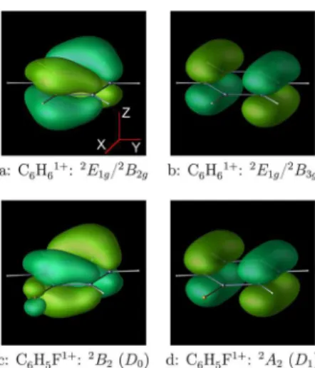
Quantum Chemical Calculations. All calculation of the crude adiabatic matrix elements as well as adiabatic force fields in C6H5F used GAMESS-US.43Geometries of the C6H6 and C6H5F neutral molecules were optimized at the RHF/cc-pVDZ-HT level. Neutral Hessians were calculated at the same level. All normal-mode frequencies reported below have not been scaled. Calculations of forces and Hessians in molecular cations utilized ROHF/cc-pVDZ-HT, at the neutral RHF/cc-pVDZ-HT geometry. Degenerate components of the2E
1gstate of C6H6+ were treated as separate 2B2g and 2B3g states in D2h symmetry (see Figure 1). In C6H5F+, the corresponding 2B2
and2A
2states are not degenerate. Calculations of nonadiabatic coupling used state-average CAS(3,2) wave functions and the cc-pVDZ-HT basis, corresponding to equally weighed ROHF solutions. Implementation of nonadiabatic coupling constants in GAMESS44does not presently support calculations at the
exact state degeneracy point. As the result, adiabatic matrix elements in C6H6 were treated separately (see below). The energy differences and the gradients of the single-state solutions agree closely with the state-averaged result. Calculations of crude adiabatic forces (eq 9) utilized ROHF/cc-pVDZ-H wave functions at the RHF/cc-pVDZ-HT geometries.
As an accuracy check, we also performed computations for the benzene cation in which the matrix elements in eqs 9 and 11 were computed directly using multireference configuration interaction (MRCI) wave functions. The underlying reference functions were determined using a CAS(3,4) computation, and averaging over the two lowest adiabatic states. The final electronic wave functions were constructed by considering dynamical correlation at the first-order MRCI level, employing the cc-pVDZ atomic basis set.
Evaluation of the requisite matrix elements is most conveniently performed using derivative couplings, which were obtained from the COLUMBUS45−47electronic structure package. The details of how these quantities were deployed to compute the elements in eqs 9 and 11, particularly the nonadiabatic coupling vector, hij, are discussed below.
Evaluation of Nonadiabatic Coupling Integrals. Evaluation of the nonadiabatic matrix elements ⟨m|ĝji(1)|n⟩(eq 11) requires some special attention. The derivative with respect to qsdoes not present a problem because
ω ω ∂ ∂ | ⟩ = − + ℏ | + ⟩ +⎜ ℏ⎟ | − ⟩ ⎛ ⎝ ⎜ ⎞ ⎠ ⎟ ⎛⎝ ⎞⎠ q n n n ( 1) n 1 n 1 2 2 s s s s s s s 1/2 1/2 (33)
reducing the result to a linear combination of matrix elements of the electronic nonadiabatic coupling ⟨Ψj|(∂/∂qs)|Ψi⟩. (In eq 33, 1sstands for a vector with 1 in the sth position and zeros in all remaining positions.) In the vicinity of the q coordinate origin, these matrix elements are given by40
⟨Ψ| ∂ ∂q |Ψ⟩ = − + − · h E E g g q ( ( ) ) j a i ji i j i j (34) = ⟨Ψ| ∂ ∂ ̂ |Ψ⟩ h q H ji j a i el (35)
where Ei is the energy of an adiabatic electronic state i at the origin and giis its gradient with respect to q. When (Ei− Ej) is large compared to ℏ1/2(g
i − gj)·ω−1/2 (in other words, when the state intersection is far away compared to a typical extent of a nuclear basis function), the denominator in eq 34 can be expanded in a Taylor series truncated at a suitably low order (we choose O(q1) to remain consistent with the quadratic expansion of the PES). The matrix elements are then evaluated in the same manner as the matrix elements of the potential.26 When the CI is present in the immediate vicinity of the origin, matrix elements of eq 34 contain an essential singularity, and Taylor expansion of the denominator is no longer appropriate. Instead, we consider a coordinate transformation
ω
= ℏ − ×
z 1/2( 1/2 q) (36)
where ω1/2 × q is understood as an element-by-element multiplication. In eq 36, matrix is unitary. It is chosen such that the first row of is in the direction of (gi− gj) × ω−1/2. The rest of is, in principle, arbitrary and can be chosen for computational convenience. By construction, transformation of eq 36 conserves the number of vibrational quanta. Therefore, a basis function |n⟩qin the q space has a finite expansion in terms of auxiliary functions |k⟩zin the z space, such that ∑ ki= ∑ ni. The expansion coefficients are Franck−Condon factors between the two spaces and can be evaluated using standard recursions.48,49 By construction, in the auxiliary z space, the coordinate dependence of eq 34 is confined to the z1 coordinate.
In order to evaluate the auxiliary matrix elements in the z space, we note that Hermite polynomials satisfy the relation
∑
= − − !! − − !! + + − − − !! = ⌊ − ⌋ − − ⌊ ⌋ H t t k k n H t k H t ( ) 2 ( 2) ( 1) ( 1 2 ) ( ) (1 ( 1) ) 2 ( 2) ( 1) ( ) k n k n k n k k 0 ( 1)/2 1 2 /2 0 (37)Therefore, multidimensional harmonic oscillator functions of eq 5 satisfy
∑
ω | ⟩ = ℏ − − − ! ! − !! − − !!| − + ⟩ + + − − − !! ! | − ⟩ = ⌊ − ⌋ ⌊ ⌋ ⎜ ⎟ ⎛ ⎝ ⎞ ⎠ ⎛ ⎝ ⎜ ⎞ ⎠ ⎟ q n s n n n s s n n n n n 1 n 1 2 ( 1) ( 1 2 ) ( 1) ( 1 2 ) (2 1) 1 ( 1) 2 ( 1) ( 1) ( ) k k s n s k k k k k n n k k k k 1/2 0 ( 1)/2 1/2 /2 1/2 k k k (38)for any k, including k = 1.
Using eq 38, we can repeatedly cancel the leading term with the denominator in eq 34, yielding a recursive expression for a one-dimensional matrix element of operator (ϵ + gq)−1 between harmonic oscillator functions, respectively, with m and n quanta
Figure 1.Dyson orbitals for the lowest ionization channels in C6H6
(a,b) and C6H5F (c,d). Note that the C6H5F figure uses a nonstandard
∑
ω δ = ⟨ | ϵ + | ⟩ = ℏ − − ϵ × − − ! ! − !! − − !! + + − − − !! ! = ⌊ − ⌋ − − − − ⌊ ⌋ ⎜ ⎟ ⎛ ⎝ ⎞ ⎠ ⎛ ⎝ ⎜ ⎞ ⎠ ⎟ I m gqn g I n s n n n s I n n 1 2 ( 1) ( ) ( 1 2 ) ( 1) ( 1 2 ) 1 ( 1) 2 ( 1) ( 1) ( ) mn s n s m n s m n s m n n 1/2 0 ( 1)/2 , 1 2 , 1 2 1/2 0 /2 1/2 (39)The same recursion relation is applicable to multidimensional matrix elements in the auxiliary z frame, provided that all quantities are understood to refer to the z1 coordinate, and integrals of the remaining degrees of freedom are replaced by δ functions of the corresponding quantum numbers.
The I00 matrix element is related to the Dawson’s integral -50 ω ω = ℏ ϵ ℏ ⎛ ⎝ ⎜ ⎞ ⎠ ⎟ ⎛ ⎝ ⎜ ⎜ ⎛ ⎝ ⎜ ⎞ ⎠ ⎟ ⎞ ⎠ ⎟ ⎟ I g g 2 00 2 1/2 2 1/2 -(40)
∫
= − z z ( ) zex z d 0 2 2 - (41)Efficient numerical implementations of Dawson’s integral are readily available.51
Calculation of the Autocorrelation Function and Surface Populations.For high expansion orders l, the formal number of terms in eq 22 grows rapidly (as O(lN) when l ≫ N, where N is the number of normal modes in the expansion). To make computation tractable, we exclude all terms involving amplitudes Ai(l−p), which differ by more than 6 vibrational quanta from any of the vibrational basis functions present in the initial wavepacket. In all cases discussed presently, increasing the cutoff to 8 quanta does not change the results.
The time series of eq 17 is only calculated for the basis functions present in the initial wavepacket. As a byproduct of the recursive eq 22, we also obtain time series expansions for other, coupled basis functions, albeit at a lower order. These expansions are used below to calculate the evolution of the total surface populations. Due to the use of different expansion orders for different basis functions within the same wavepacket, this procedure yields only an estimation of the total surface population, which may lose significance at an earlier time than the matching autocorrelation function. We monitor this significance loss by observing the total wavepacket norm, obtained from the same time series.
■
RESULTS AND DISCUSSIONFor numerical calculations of short-time autocorrelation functions, we consider two molecules of current experimental interest, benzene C6H6and fluorobenzene C6H5F. In benzene, the initial cation is created directly at the seam of the CI between the two branches of the 2E
1g state. Previous studies have shown the Jahn−Teller distorted minimum to correspond to the 2B
3g state, whereas the minimum on the 2B2g surface corresponds to a first-order saddle point connecting the symmetry-equivalent minima (see, e.g., refs 52 and 53 and references therein.) In fluorobenzene, the two lowest cationic states, D0 (2B2) and D1 (2A2) are nondegenerate but are separated by only 0.35 eV.
In intense low-frequency fields, molecular cations are produced through tunneling ionization.5 For degenerate
(C6H6) and nearly degenerate (C6H5F) target states, relative ionization yields are determined primarily by the nodal structure of the Dyson orbital describing the ionization event;54the proximity of nodal planes to the field polarization
direction suppresses ionization.
For example, for laser field in the X direction (Figure 1), strong-field ionization of C6H6will preferentially populate the B2g electronic surface (panel a). In C6H5F, the ground state (D0, 2B2) will be populated preferentially. For other field polarizations (e.g., Z), tunneling ionization may form a coherent vibronic wavepacket, spanning both surfaces. In such cases, detailed simulations are necessary to determine the initial wavepacket composition.54For simplicity, here, we limit ourselves to the case of the initial wavepacket dominated by one of the electronic surfaces.
Benzene C6H6. The calculated square modulus of the nuclear autocorrelation function in C6H6is shown in Figure 2.
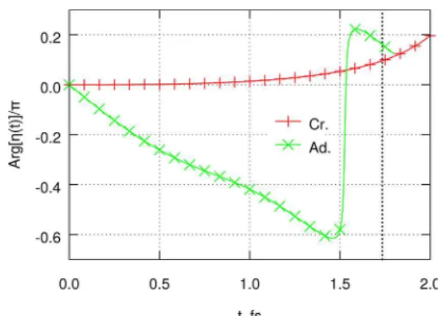
For both choices of the electronic ansatz (crude adiabatic versus adiabatic), decay of the autocorrelation function is nearly Gaussian in time. Superficially, there is also qualitative similarity between the two curves, with the crude adiabatic result decaying to 0.5 by ∼0.86 fs. The adiabatic autocorrelation function reaches 0.5 by 0.45 fs. In both cases, the decay is fast on the laser-cycle time scale, with emission fully suppressed at the harmonic cutoff of the 800 nm driving field. The two results thus may be hard to distinguish experimentally, especially at longer wavelengths. At the same time, examination of the calculated phase of the nuclear autocorrelation function (Figure 3) reveals the similarity as a numerical accident. Indeed, within the adiabatic ansatz, the phase initially grows linearly with time (green line in Figure 3). This is the expected behavior for an
Figure 2.Square modulus of the nuclear autocorrelation function in C6H6+. The initial wavepacket is a replica of the ground-state
vibrational state of neutral C6H6, placed on the branch of the E1gstate
correlating to B2g in D2h symmetry. Decay of the initial population
placed on the B3gbranch is indistinguishable on the present time scale
and is not shown. Red plus signs: Crude adiabatic electronic wave functions (N = 120). Green crosses: Adiabatic electronic wave functions (N = 80). Blue line: Gaussian fit to adiabatic |η|2at the time
origin. The curves continue to the time t where order-(N − 2) expansion begins to deviate from the order-N result. Solid lines of matching color are calculated from eq 30, fitted to the first three even derivatives of the autocorrelation function. Vertical dotted line corresponds to cutoff harmonics for the 800 nm (t = 1.73 fs) driving IR field.
initially stationary wavepacket being accelerated by a constant force.9 This acceleration drives the decrease in the autocorrelation magnitude.9,26
In contrast, within the crude adiabatic ansatz (red line), the phase remains zero during the initial ∼1.5 fs, indicating that the nuclei remain stationary on the initially populated surface. Instead, the decrease in the autocorrelation magnitude is driven by a transition to the coupled electronic surface (B3gsymmetry at D6h). This behavior can be clearly seen in the time dependence of the electronic surface populations (Figure 4).
The crude adiabatic population on the initially populated B2g surface decreases rapidly, with nearly half of the population transferred onto the coupled surface in only 1.4 fs. If coupling between the surfaces is disabled in the crude adiabatic simulation, the decay of the autocorrelation function is slowed dramatically, with |η|2reaching 0.5 only at ∼3 fs (not shown). Because gradient terms in the autocorrelation decay (eq 7 of ref 26; here, we do not separate out terms by order of the potential in eq 9) are very similar between the adiabatic and crude adiabatic simulations, the difference clearly lies in the quadratic terms (eq 8 of ref 26); these terms are present in the adiabatic simulation but are neglected for our choice of the crude adiabatic ansatz.
Overall, the apparently somewhat reasonable performance of the crude adiabatic simulation for the C6H6+ autocorrelation decay comes from two major, mutually compensating deficiencies, (a) underestimation of the decay rate on the initially populated surface due to the lack of quadratic coupling terms and (b) gross overestimation of the surface crossing rate. Returning to the adiabatic autocorrelation decay (green crosses, Figure 2), we notice that while at very short times (≤0.6 fs) it decays nearly as a Gaussian, marked deviations from simple Gaussian decay appear at later time. Between 0.7 and 1.3 fs, the autocorrelation function appears to be linear in time, while the beginning of a revival is seen at 1.6 fs. The revival feature does not appear to be a numerical artifact; it first appears in an order-50 expansion (eq 17), remaining present as the expansion order is increased to 80. Although the apparent revival of the autocorrelation function is at the harmonics cutoff for the 800 nm driving field, it is well within the plateau for λ ≥ 1.2 μm. The revival-like feature also appears to be associated with a 0.8π phase jump of the autocorrelation function (Figure 3), providing a signature that should be clearly visible in quantum-path interference experiments.23 We note that the
population of the B2g adiabatic surfaces appears to reach a minimum at t ≈ 1.4 fs, nearly simultaneously with the beginning of the phase jump. Because an identical minimum in the autocorrelation function appears in single-surface simulations (see below), the population minimum is likely coincidental.
It would have been very interesting to further explore and characterize this feature of the autocorrelation function. Unfortunately, our Taylor expansion (eq 17) loses all significance beyond order 80 and cannot be employed for t ≥1.75 fs in C6H6+.
It is instructive to examine the relative importance of different terms in eq 8 that give rise to the time evolution of the adiabatic autocorrelation function. Due to the presence of inversion symmetry, laser coupling (eq 10) plays no role in C6H6+ dynamics. However, all remaining terms are potentially significant. The easiest term to grasp intuitively is the same-surface gradient coupling, which contributes to eq 9. This term represents a constant force along one of the normal modes, which accelerates the initial wavepacket away from the origin. Large gradients along soft normal modes are effective at inducing nuclear dynamics. In C6H6+, modes of e2g symmetry are particularly active, including the Jahn−Teller active in-plane skeletal deformation ω18 mode (∼600 cm−1) and the out-of-plane H-wagging ω17mode (∼1180 cm−1). However, no single mode dominates in the description of the autocorrelation function, with 10 distinct modes comprising the leading contributions. The second contribution in the same-surface dynamics is due to the curvature (Hessian) terms, again forming a part of eq 9. These terms can be diagonal, resulting in spread or compaction of the wavepacket along the correspond-ing normal mode, or off-diagonal, which induces the wave-packet to “change direction”. In C6H6+, diagonal terms are most important, in particular, along the various out-of-plane H-wag modes (ω4, ω11, and ω19). However, a numerically converged description of the dynamics required the inclusion of over 100 Hessian couplings. Similarly, no single nonadiabatic term, which gives rise to the population transfer between the adiabatic states, is clearly dominant. For example, matrix elements of the operator in eq 34 are of similar magnitude for four distinct normal modes, involving excitation (or de-excitation) of the ω8, ω11, ω19, and ω20, which are generally
Figure 3.Phase of the nuclear autocorrelation function in C6H6+. Red
plus signs: Crude adiabatic. Green crosses: Adiabatic. Also see the Figure 2 caption.
Figure 4.Estimation of the fraction of the wavepacket on the initially populated surface in C6H6+. Red plus signs: Crude adiabatic, D0. Green
crosses: Adiabatic, D0. The estimated adiabatic surface population
loses significance at t = 1.60 fs and is truncated at this point. Also see the Figure 2 caption.
out-of-plane ring deformations and H-wagging modes. (The actual matrix elements of ĝji(1) are further modulated by the quantum numbers and mode frequencies; see eq 33.) Four more modes are nearly as active for nonadiabatic population transfer and must be included in numerical simulations as well. Taken together, the gradient, Hessian, and nonadiabatic coupling terms rapidly couple the initial vibronic wave function to many vibrational coordinates, encompassing more than half of the normal modes within the first few femtoseconds.
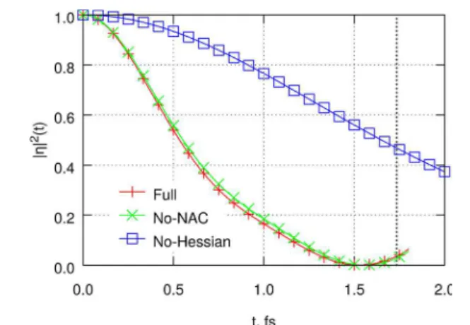
Even though both the same-surface and nonadiabatic couplings are important for the short-time wavepacket and surface population evolution, the same is not true for the autocorrelation function (Figure 5). Autocorrelation presents a
very strong filter of the overall wavepacket, with only the population of the initial |0⟩ function being significant. In C6H6+, the |0⟩|Ψb2g⟩ basis function has only one, moderate non-adiabatic coupling (∼0.002 au to |ω18⟩|Ψb3g⟩), with all other nonadiabatic terms smaller by an order of magnitude or more. Although nonadiabatic coupling becomes much stronger and more diverse for other basis functions, these couplings affect |η|2only indirectly by removing the population from the initially coupled same-surface modes. It is therefore not entirely surprising that the full, two-surface autocorrelation function (red line, Figure 5) is nearly indistinguishable from the single-surface autocorrelation (green line), despite substantial population transfer to the B3g surface. In contrast, the initial | 0⟩|Ψb2g⟩state is directly coupled to many other modes through the Hessian term in eq 9. Removing this term from the simulation (blue line, Figure 5) leads to a dramatic change in the results.
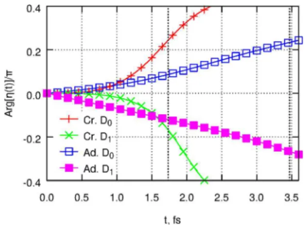
Fluorobenzene C6H5F.Results for the nuclear autocorre-lation function in fluorobenzene are collected in Figures 6 (square norm of the autocorrelation function), 7 (weight of the initially populated surface), and 8 (phase of the autocorrelation function).
As seen above for C6H6+, the crude adiabatic ansatz suffers from overestimation of population transfer between coupled electronic surfaces (Figure 7) and underestimation of the extent of same-surface wavepacket evolution, as seen from the nearly zero phase of the autocorrelation function up to 1 fs (Figure 8). Unlike the benzene case, these two deficiencies no longer partially compensate for each other, so that the crude adiabatic result for the magnitude of the autocorrelation function is now
in a significantly worse agreement with the more rigorous adiabatic result (Figure 6). Overall, it is clear that the crude adiabatic wave function ansatz, in its simplest form used presently, is not useful for modeling short-time autocorrelation functions. Therefore, we will not discuss the crude adiabatic results any further.
In C6H5F+, the two lowest electronic states are separated by ∼0.35 eV at the neutral species geometry. It is therefore possible to evaluate matrix elements of eq 34 using either the Taylor expansion of the denominator or the (exact but expensive) reduction to integrals of eq 39. Within the resolution of the graphs in Figures 6−8, the results are indistinguishable.
Given that the starting point of the dynamics in C6H5F+is no longer directly at the CI, it is not entirely surprising that the autocorrelation functions now decay at a rate more
character-Figure 5. Contributions to the magnitude of the nuclear autocorrelation function in C6H6+. Red line: Full calculation. Green
line: Excluding the nonadiabatic coupling terms of eq 11. Blue line: Linear coupling terms only in eq 9. Also see the Figure 2 caption.
Figure 6.Square modulus of the nuclear autocorrelation function in C6H5F+. The initial wavepacket is a replica of the ground-state
vibrational state of neutral C6H5F, placed on the D0(B2) or D1(A2)
electronic surface of the cation. Red plus signs: Crude adiabatic, D0(N
= 120). Green crosses: Crude adiabatic, D1 (N = 120). Blue open
squares: Adiabatic, D0(N = 90). Magenta filled squares: Adiabatic, D1
(N = 90). The curves continue to the time t where order-(N − 2) expansion begins to deviate from the order-N result. Solid lines of matching color are calculated from eq 30, fitted to the first three even derivatives of the autocorrelation function. The fit for the crude adiabatic D0curve grows unboundedly and has been truncated after
1.7 fs. Vertical dotted lines correspond to cutoff harmonics for the 800 nm (t = 1.73 fs) and 1600 nm (t = 3.46 fs) driving IR fields.
Figure 7.Estimation of the fraction of the wavepacket on the initially populated surface in C6H5F+. Red plus signs: Crude adiabatic, D0.
Green crosses: Crude adiabatic, D1. Blue open squares: Adiabatic, D0.
istic of “normal”, electronically nondegenerate cations. Nuclear motion in this cation suppresses harmonic efficiency by only ∼50% for the cutoff harmonics of the 800 nm driving field. Even at the cutoff of the 1.6 μm harmonics, the |η|2values are still close to 15%, similar to the behavior seen in O2+ and PF3+.26
The nearly single-surface nature of the dynamics at short times is also evident from the surface populations (Figure 7). For the initial population placed on the ground electronic surface (blue open squares), population of the D0surface drops to ∼0.95 at 2.5 fs, before recovering to near-unity at later times. For the D1surface, 90% of the population remains on the same surface for the first 1.8 fs (the cutoff harmonics of the 800 nm driving field) and only starts to significantly decay to D0at later times.
As was already seen above for C6H6+, even the substantial (>30%) population transfer at later times remains “invisible” in the autocorrelation. At least up to 3.5 fs, the magnitude of the autocorrelation function remains nearly the same for the initial populations placed on either D0 or D1 surfaces (Figure 6). However, the phases of the two autocorrelation functions are of opposite sign and are nearly identical in magnitude (Figure 8). This phase is mapped directly onto the phase of the emitted harmonics. Both ionization channels are accessible through tunneling ionization, with the relative initial populations and phases controlled by the polarization direction of the ionizing field. Therefore, it should in principle be possible to use channel interference in C6H5F for controlling the atto-chirp of the emitted harmonics and hence for shaping attosecond pulses.
Finally, the presence of laser−dipole coupling terms in eq 22 potentially makes the dynamics sensitive to the presence of the intense laser field. The two possible effects are field-induced subcycle electronic transitions and modulation of the state energy separation through the linear Stark effect. Unfortunately, the difference in the permanent dipole moments of the two states in C6H5F+ is only ∼0.06 e-Bohr. The transition dipole between the two states is also small (∼0.27 e-Bohr). On the short time scales considered here, incorporation of either effect does not change the results appreciably.
Similar to the case of C6H6+ above, no single normal mode dominates the short-time evolution of the initial wavepacket in
C6H5F+. For the D0 (2B2) state, more than 10 gradient terms are required for converged same-surface dynamics. The most prominent contributions come from a1 modes, including the ω11(∼560 cm−1, unscaled) skeletal in-plane bending mode, ω
7 (∼1260 cm−1) in-plane o-,m-H wagging mode, and ω4(∼1790 cm−1) in-plane skeletal stretching mode. Approximately 150 couplings are numerically important for the Hessian terms, with the diagonal terms due to the ω14 (∼460 cm−1) a2 skeletal screw-twisting mode and ω17(∼1780 cm−1) b2in-plane skeletal stretch modes being the most prominent. Unlike the C6H6+ case, an off-diagonal coupling involving a “hexane-chair-like” mode (ω28, ∼760 cm−1, b2) and a “leaf-folding” mode around the F−(i-C)−(p-C) axis (ω29, ∼560 cm−1, b2) is also very strong. The nonadiabatic coupling in C6H5F+ is dominated by b1vibrational modes, with the in-plane skeletal bending modes (ω23, ∼670; ω17, ∼1780 cm−1) being the most prominent. Despite slower dynamics, the qualitative picture of the initial wavepacket being “torn apart” by the nearby CI remains valid in C6H5F as well.
■
CONCLUSIONSIn this work, we developed a simple, numerically tractable approach for calculating short-time autocorrelation functions for nuclear dynamics in the vicinity of CIs. Accurate description of the PESs, at least through the second order in coordinate displacements, is essential for the prediction of autocorrelation functions in such systems. Taken alone, linear terms in the potential account for less than half of the autocorrelation decay. Nonadiabatic coupling is critical for the short-time dynamics of wavepackets created directly at a CI (such as in C6H6). However, due to the strong filter property of the autocorrelation function, the nonadiabatic term may become “invisible” in same-electronic-surface HHG. The C6H6+ cation provides such an example, where the |0⟩|Ψb2g⟩autocorrelation lacks a discernible signature of the (clearly present) non-adiabatic dynamics.
The same-surface nuclear dynamics at the CI in C6H6+ manifests itself at short times (0.7−1.5 fs) as sub-Gaussian decay of the autocorrelation function and possibly as an autocorrelation revival. The presence and characteristics of such a revival would need to be confirmed by detailed time-dependent wavepacket simulations, which are currently under-way. If the revival persists, HHG experiments on aligned C6H6 (or similar) molecules would provide a unique opportunity of experimentally dissecting dynamics at a CI, at its natural time scale. These dynamics may be more readily observable in the phase of harmonic emission rather than in its magnitude.
Even though the simplest, single-channel HHG mechanism in both C6H6and C6H5F is “blind” to nonadiabatic dynamics, they may still manifest themselves in cross-channel contribu-tions8,10,13 to HHG. Previously, multichannel HHG contribu-tions were identified in harmonics intensity,8 phase,8,10 polarization,8 and ellipticity.55 The interchannel interference
requires coherence to exist between two intermediate states of the ion. This coherence can be created by the initial strong-field ionization,8,13,55subcycle field-driven electronic transitions,55or
electron correlation.56−58 Electronic transitions due to non-adiabatic molecular dynamics should manifest themselves in similar multichannel effects. Modeling of the nuclear contributions to multichannel HHG can no longer be separated from the description of the field-driven electron dynamics in the continuum13and is outside the scope of this work.
Figure 8.Phase of the nuclear autocorrelation function in C6H5F+.
Red plus signs: Crude adiabatic, initial wavepacket on D0. Green
crosses: Crude adiabatic, initial wavepacket on D1. Blue open squares:
Adiabatic, D0. Magenta filled squares: Adiabatic, D1. For each curve,
the energy origin is chosen such that the electronic contribution to the phase vanishes. Also see the Figure 6 caption.
When the electronic degeneracy at the initial position is lifted by as little as 0.3 eV (C6H5F), nonadiabatic coupling plays almost no role during the first 2 fs of dynamics, increasing in importance at later times. For the isolated-surface dynamics, the essence of the autocorrelation function decay is captured nearly quantitatively by a simple three-parameter fit (eq 30). Because strong-field ionization populates nearly degenerate electronic states coherently and potentially with similar efficiency, multichannel interference can still lead to nontrivial effects in HHG spectroscopy, even in the absence of significant nonadiabatic dynamics. Nuclear dynamics in such nearly degenerate systems may also prove useful in shaping attosecond pulses.
■
AUTHOR INFORMATION Corresponding Author*E-mail: [email protected].
Notes
The authors declare no competing financial interest.
■
REFERENCES(1) Ferray, M.; L’Huillier, A.; Li, X. F.; Lompre, L. A.; Mainfray, G.; Manus, C. Multiple-harmonic conversion of 1064 nm radiation in rare gases. J. Phys. B 1988, 21, L31−L35.
(2) Popmintchev, T.; Chen, M.-C.; Popmintchev, D.; Arpin, P.; Brown, S.; Ališauskas, S.; Andriukaitis, G.; Balc̆iunas, T.; Mücke, O. D.; Pugzlys, A.; et al. Bright coherent ultrahigh harmonics in the keV X-ray regime from mid-infrared femtosecond lasers. Science 2012, 336, 1287−1291.
(3) Corkum, P. B. Plasma perspective on strong field multiphoton ionization. Phys. Rev. Lett. 1993, 71, 1994−1997.
(4) Lewenstein, M.; Balcou, P.; Ivanov, M. Y.; L’Huillier, A.; Corkum, P. B. Theory of high-harmonic generation by low-frequency laser fields. Phys. Rev. A 1994, 49, 2117−2132.
(5) Krausz, F.; Ivanov, M. Attosecond physics. Rev. Mod. Phys. 2009,
81, 164−234.
(6) Salières, P.; Maquet, A.; Haessler, S.; Caillat, J.; Taïeb, R. Imaging orbitals with attosecond and Ångström resolutions: Toward attochemistry? Rep. Prog. Phys. 2012, 75, 062401.
(7) Ivanov, M. Y.; Brabec, T.; Burnett, N. Coulomb corrections and polarization effects in high-intensity high-harmonic emission. Phys.
Rev. A 1996, 54, 742−745.
(8) Smirnova, O.; Mairesse, Y.; Patchkovskii, S.; Dudovich, N.; Villeneuve, D.; Corkum, P.; Ivanov, M. Y. High harmonic interferometry of multi-electron dynamics in molecules. Nature 2009, 460, 972−977.
(9) Haessler, S.; Boutu, W.; Stankiewicz, M.; Frasinski, L. J.; Weber, S.; Caillat, J.; Taïeb, R.; Maquet, A.; Breger, P.; Monchicourt, P.; et al. Attosecond chirp-encoded dynamics of light nuclei. J. Phys. B 2009, 42, 134002.
(10) Smirnova, O.; Patchkovskii, S.; Mairesse, Y.; Dudovich, N.; Villeneuve, D.; Corkum, P.; Ivanov, M. Y. Attosecond circular dichroism spectroscopy of polyatomic molecules. Phys. Rev. Lett. 2009, 102, 063601.
(11) Diveki, Z.; Camper, A.; Haessler, S.; Auguste, T.; Ruchon, T.; Carré, B.; Salières, P.; Guichard, R.; Caillat, J.; Maquet, A.; et al. Spectrally resolved multi-channel contributions to the harmonic emission in N2. New J. Phys. 2012, 14, 023062.
(12) Itatani, J.; Levesque, J.; Zeidler, D.; Niikura, H.; Pépin, H.; Kieffer, J. C.; Corkum, P. B.; Villeneuve, D. M. Tomographic imaging of molecular orbitals. Nature 2004, 432, 867−871.
(13) Smirnova, O.; Patchkovskii, S.; Mairesse, Y.; Dudovich, N.; Ivanov, M. Y. Strong-field control and spectroscopy of attosecond electron-hole dynamics in molecules. Proc. Natl. Acad. Sci. U.S.A. 2009,
106, 16556−16561.
(14) Wagner, N. L.; Wüest, A.; Christov, I. P.; Popmintchev, T.; Zhou, X.; Murnane, M. M.; Kapteyn, H. C. Monitoring molecular
dynamics using coherent electrons from high harmonic generation.
Proc. Natl. Acad. Sci. U.S.A. 2006, 103, 13279−13285.
(15) Shafir, D.; Soifer, H.; Bruner, B. D.; Dagan, M.; Mairesse, Y.; Patchkovskii, S.; Ivanov, M. Y.; Smirnova, O.; Dudovich, N. Resolving the time when an electron exits a tunnelling barrier. Nature 2012, 485, 343−346.
(16) Shiner, A. D.; Schmidt, B. E.; Trallero-Herrero, C.; Wörner, H. J.; Patchkovskii, S.; Corkum, P. B.; Kieffer, J.-C.; Légaré, F.; Villeneuve, D. M. Probing collective multi-electron dynamics in xenon with high-harmonic spectroscopy. Nat. Phys. 2011, 7, 464−467.
(17) Leeuwenburgh, J.; Cooper, B.; Averbukh, V.; Marangos, J. P.; Ivanov, M. High-order harmonic generation spectroscopy of correlation-driven electron hole dynamics. Phys. Rev. Lett. 2013, 111, 123002.
(18) Ivanov, M.; Smirnova, O. Opportunities for sub-laser-cycle spectroscopy in condensed phase. Chem. Phys. 2013, 414, 3−9.
(19) Baker, S.; Robinson, J. S.; Haworth, C. A.; Teng, H.; Smith, R. A.; Chirilă, C. C.; Lein, M.; Tisch, J. W. G.; Marangos, J. P. Probing proton dynamics in molecules on an attosecond time scale. Science 2006, 312, 424−427.
(20) Baker, S.; Robinson, J. S.; Lein, M.; Chirilă, C. C.; Torres, R.; Bandulet, H. C.; Comtois, D.; Kieffer, J. C.; Villeneuve, D. M.; Tisch, J. W. G.; et al. Dynamic two-center interference in high-order harmonic generation from molecules with attosecond nuclear motion. Phys. Rev.
Lett. 2008, 101, 053901.
(21) Farrell, J. P.; Petretti, S.; Förster, J.; McFarland, B. K.; Spector, L. S.; Vanne, Y. V.; Decleva, P.; Bucksbaum, P. H.; Saenz, A.; Gühr, M. Strong field ionization to multiple electronic states in water. Phys. Rev.
Lett. 2011, 107, 083001.
(22) Bredtmann, T.; Chelkowski, S.; Bandrauk, A. D. Effect of nuclear motion on molecular high order harmonic pump probe spectroscopy. J. Phys. Chem. A 2012, 116, 11398−11405.
(23) Zaïr, A.; Siegel, T.; Sukiasyan, S.; Risoud, F.; Brugnera, L.; Hutchison, C.; Diveki, Z.; Auguste, T.; Tisch, J. W.; Salières, P.; et al. Molecular internal dynamics studied by quantum path interferences in high order harmonic generation. Chem. Phys. 2013, 414, 184−191.
(24) Lein, M. Attosecond probing of vibrational dynamics with high-harmonic generation. Phys. Rev. Lett. 2005, 94, 053004.
(25) Le, A.-T.; Morishita, T.; Lucchese, R. R.; Lin, C. D. Theory of high harmonic generation for probing time-resolved large-amplitude molecular vibrations with ultrashort intense lasers. Phys. Rev. Lett. 2012, 109, 203004.
(26) Patchkovskii, S. Nuclear dynamics in polyatomic molecules and high-order harmonic generation. Phys. Rev. Lett. 2009, 102, 253602.
(27) Falge, M.; Engel, V.; Lein, M. Vibrational-state and isotope dependence of high-order harmonic generation in water molecules.
Phys. Rev. A 2010, 81, 023412.
(28) Madsen, C. B.; Abu-samha, M.; Madsen, L. B. High-order harmonic generation from polyatomic molecules including nuclear motion and a nuclear modes analysis. Phys. Rev. A 2010, 81, 043413. (29) Förster, J.; Saenz, A. Theoretical study of the inversion motion of the ammonia cation with subfemtosecond resolution for high-harmonic spectroscopy. ChemPhysChem 2013, 14, 1438−1444.
(30) Domcke, W., Yarkony, D. R., Köppel, H., Eds. Conical
Intersections: Electronic Structure, Dynamics and Spectroscopy; World
Scientific: Singapore, 2004.
(31) Walters, Z. B.; Tonzani, S.; Greene, C. H. High harmonic generation in SF6: Raman-excited vibrational quantum beats. J. Phys. B
2007, 40, F277−F283.
(32) Walters, Z. B.; Tonzani, S.; Greene, C. H. Vibrational interference of Raman and high harmonic generation pathways.
Chem. Phys. 2009, 366, 103−114.
(33) We use the operator notation to emphasize that ĝ(1) is a
differential operator, rather than simple multiplicative potentials appearing in the remaining terms in eq 8.
(34) Yarkony, D. R. In Conical Intersections: Electronic Structure,
Dynamics and Spectroscopy; Domcke, W., Yarkony, D. R., Köppel, H.,
(35) Chirilă, C. C.; Lein, M. Effect of dressing on high-order harmonic generation in vibrating H2molecules. Phys. Rev. A 2008, 77,
043403.
(36) Longuet-Higgins, H. In Advances in Spectroscopy; Thompson, H. W., Ed.; Interscience Publishers: New York, 1961; Vol. 2; pp 429−472. (37) Higher-order coordinate dependence of the eq 9 potentials is beyond the accuracy of the crude adiabatic ansatz as written presently and must be neglected.
(38) Atabek, O.; Hardisson, A.; Lefebre, R. On the crude adiabatic molecular vibronic states and their use in the interpretation of radiationless processes in molecules. Chem. Phys. Lett. 1973, 20, 40− 44.
(39) Johnson, W. C., Jr.; Weigang, O. E., Jr. Theory of vibronic interactions: The importance of floating basis sets. J. Chem. Phys. 1975,
63, 2135−2143.
(40) Köppel, H.; Domcke, W.; Cederbaum, L. S. Multimode molecular dynamics beyond the Born−Oppenheimer approximation.
Adv. Chem. Phys. 1984, 57, 59−246.
(41) Pulay, P. Ab initio calculation of force constants and equilibrium geometries in polyatomic molecules. Mol. Phys. 1969, 17, 197−204.
(42) Dunning, T. H. Gaussian basis sets for use in correlated molecular calculations. I. The atoms boron through neon and hydrogen. J. Chem. Phys. 1989, 90, 1007−1023.
(43) Schmidt, M. W.; Baldridge, K. K.; Boatz, J. A.; Elbert, S. T.; Gordon, M. S.; Jensen, J. H.; Koseki, S.; Matsunaga, N.; Nguyen, K. A.; Su, S.; et al. General atomic and molecular electronic structure system.
J. Comput. Chem. 1993, 14, 1347−1363.
(44) Dudley, T. J.; Olson, R. M.; Schmidt, M. W.; Gordon, M. S. Parallel coupled perturbed CASSCF equations and analytic CASSCF second derivatives. J. Comput. Chem. 2006, 27, 352−362.
(45) Lengsfield, B. H., III; Saxe, P.; Yarkony, D. R. On the evaluation of nonadiabatic coupling matrix elements using SA-MCSCF/CI wave functions and analytic gradient methods. I. J. Chem. Phys. 1984, 81, 4549−4553.
(46) Lischka, H.; Shepard, R.; Pitzer, R. M.; Shavitt, I.; Dallos, M.; Müller, T.; Szalay, P. G.; Seth, M.; Kedziora, G. S.; Yabushita, S.; et al. High-level multireference methods in the quantum-chemistry program system COLUMBUS: Analytic MR-CISD and MR-AQCC gradients and MR-AQCC-LRT for excited states, GUGA spin−orbit CI and parallel CI density. Phys. Chem. Chem. Phys. 2001, 3, 664−673.
(47) Lischka, H.; Dallos, M.; Szalay, P. G.; Yarkony, D. R.; Shepard, R. Analytic evaluation of nonadiabatic coupling terms at the MR-CI level. I. Formalism. J. Chem. Phys. 2004, 120, 7322−7329.
(48) Doktorov, E.; Malkin, I.; Man’ko, V. Dynamical symmetry of vibronic transitions in polyatomic molecules and the Franck−Condon principle. J. Mol. Spectrosc. 1977, 64, 302−326.
(49) Gruner, D.; Brumer, P. Efficient evaluation of harmonic polyatomic Franck−Condon factors. Chem. Phys. Lett. 1987, 138, 310−314.
(50) Abramowitz, M.; Stegun, I. A. Handbook of Mathematical
Functions: With Formulas, Graphs, And Mathematical Tables; Dover
Publications: New York, 1964.
(51) Rybicki, G. B. Dawson’s integral and the sampling theorem.
Comput. Phys. 1989, 3, 85−87.
(52) Johnson, P. M. The Jahn−Teller effect in the lower electronic states of benzene cation. I. Calculation of linear parameters for the e2g
modes. J. Chem. Phys. 2002, 117, 9991−10000.
(53) Applegate, B. E.; Miller, T. A. Calculation of the Jahn−Teller effect in benzene cation: Application to spectral analysis. J. Chem. Phys. 2002, 117, 10654−10674.
(54) Spanner, M.; Patchkovskii, S. One-electron ionization of multielectron systems in strong nonresonant laser fields. Phys. Rev. A 2009, 80, 063411.
(55) Mairesse, Y.; Higuet, J.; Dudovich, N.; Shafir, D.; Fabre, B.; Mével, E.; Constant, E.; Patchkovskii, S.; Walters, Z.; Ivanov, M. Y.; et al. High harmonic spectroscopy of multichannel dynamics in strong-field ionization. Phys. Rev. Lett. 2010, 104, 213601.
(56) Walters, Z. B.; Smirnova, O. Attosecond correlation dynamics during electron tunnelling from molecules. J. Phys. B 2010, 43, 161002.
(57) Patchkovskii, S.; Smirnova, O.; Spanner, M. Attosecond control of electron correlations in one-photon ionization and recombination. J.
Phys. B 2012, 45, 131002.
(58) Torlina, L.; Ivanov, M.; Walters, Z. B.; Smirnova, O. Time-dependent analytical R-matrix approach for strong-field dynamics. II. Many-electron systems. Phys. Rev. A 2012, 86, 043409.