ATMOSPHERIC GRAVITY WAVES, AN OBSERVATIONAL AND NUMERICAL STUDY
by
GEORGE J. BOER
B.Sc., University of British Columbia (1963)
M.A., University of Toronto (1965)
SUBMITTED IN PARTIAL FULFILLMENT OF THE REQUIREMENTS FOR THE DEGREE OF
DOCTOR OF PHILOSOPHY
at the
MASSACHUSETTS INSTITUTE OF TECHNOLOGY June 22, 1970
Signature of Author ... . .. .. . Department of Meteorology, 22 June 1970
Certified by ...0 . ... Thesis Supervisor
Accepted by ...
Chairman, Depart entgtl Committee on Graduate Students
N
N'
ATMOSPHERIC GRAVITY WAVES, AN OBSERVATIONAL AND NUMERICAL STUDY
by
GEORGE J. BOER
Submitted to the Department of Meteorology on June 22, 1970 in partial fulfillment of the requirements for the degree of Doctor of Philosophy.
ABSTRACT
Two topics concerning gravity wave motions in the atmosphere are discussed. The first topic concerns the propagation of the waves through regions of varying wind shear and the second topic concerns the detection and measurement of gravity wave motions in the upper atmosphere.
The linear theory of gravity wave motions for a two dimensional, non-rotating, inviscid, adiabatically moving hydrostatic atmosphere
is reviewed. A numerical model for the equations is obtained and integrated as an initial and boundary value problem for wave motions with a fixed horizontal wavelength. The behavior of the wave motions
for different distributions of the mean wind for which a critical level exists is obtained.
The non-linear approach to the equations of motion in terms of the perturbation equations is discussed and it is shown that no reso-nant interactions between simple waves is possible in the .atmosphere unlike the case for internal waves in the ocean.
The numerical model is extended to include directly the interac-tion of the wave mointerac-tions and the mean flow. It is found that the region of accelerated mean flow depends on the initial profile of the mean flow and that a shearing region is produced in the mean flow which descends with time and for which the magnitude of the shear
increases until the Richardson stability condition is violated. The behavior of the wave motions at a critical level becomes quite differ-ent from that deduced from linear theory as time goes on.
The observational aspect of the study involves the detection and measurement of gravity wave motions in the atmosphere in the 30-60km region. Data obtained by the ROBIN falling sphere method and the smoke trail method are analysed. The ROBIN experiment permitted the evaluation of the errors involved in the measurements as each falling sphere was tracked separately by two radars. The data is reduced by a method which gives a uniform response with height unlike the usual reduction procedure. The spectrum of the velocity profile in the-ver-tical is obtained and found to be similar to that obtained for motions at lower levels. The experiment also permits an estimate of the hor-izontal and time scales to be made so that the motions may be compared with simple gravity wave theory.
The smoke trail experiment has not been previously used in the 30-60 km region. Despite difficulties in the data reduction it is pos-sible to obtain velocity profiles and to estimate the error involved. The method offers promise if the observational conditions can be
op-timized. The spectra of the velocity profiles in the vertical are ob-tained and are found to differ from those obob-tained in the ROBIN exper-iment. The horizontal scale of the motions is also estimated.
Thesis Supervisor: Reginald E. Newell Title: Professor of Meteorology
Table of Contents Abstract... 2 Table of Contents... 4 List of Figures... 6 List of Tables... 8 Acknowledgement...9 1.0 Introduction... 10
2.0 Theoretical and numerical results for the hydrostatic gravity wave... 18
2.1 The equations of motion and results for linear theory, 18 2.1.0 Approximations to the equations... .19
2.1.1 The energy equations... 20
2.1.2 The equations in coordinates... 21
2.1.3 The perturbation equations... 25
2.1.4 The conservation of energy for the perturbation equations... ... .. o2 2.1.5 Simple plane wave solutions... 29
2.1,6 Variable background conditions... 31
2.2 A linear numerical model... 39
2.2.1 Results of calculations for the linear model.... 46
2.3 Non-linear effects...,... ... 65
2.3.1 The perturbation approach... ... 65
2.3.2 A numerical approach to non-linear wave motions. 72 2.3.3 The interaction of the mean flow and one Fourier component... ... 73
2.3.4 Results of calculations for one Fourier component... ... 75
3.0 Observations of gravity waves in the upper atmosphere... 94
3..1 The ROBIN experiment ... ,... 96
3.1.1 Data reduction...99
3.1.2 Calculation of smoothed velocities...100
3.1.3 Smoothing and the accuracy of soundings...105
3.1.4 Smoothing
and
the variance of soundings...1063.1.5 Smoothing and correlation...108
3.1.6 Spectra and the vertical scale of the motions..l12 3.1.7 The horizontal scale of the motions...114
3.1.9 Relation of deduced scales and the theoretical
frequency equation...118
3.1.10 Summary of results...120
3.2 The measurement of velocities in the 30-60 km region by means of smoke trails...121
3.2.1 The smoke trail system...121
3.2.2 Data reduction procedures...123
3.2.3 Velocity profiles...127
3.2.4 Analysis of the velocity profiles...135
3.2.5 Summary of results...141
3.3 Comparison of methods and the problem of gravity wave measurement.. ... . ... 142
4.0 Concluding remarks...145
Appendix I, Neglect of rotation for gravity wave motions...148
Bibliography and References...151
List of Figures
2.1 Finite difference grid for the linearized equations... 43 2.2 The vertical profile of at ui at 3 hours... 48
.E.3 The vertical profile of 0a4for the case of a mean wind which increases linearly with height... 51
2.4 The vertical distribution of the momentum flux term for the case of a mean wind which increases linearly with
height.. . . .. . ... 000 00 00 00 00 52 2.5a The vertical profile of
LA
for the case of a timedependent mean wind.,...,... 54 2.5b The vertical distribution of the momentum flux term for
the case of a time dependent mean wind... 55 2.6 Time dependent behaviour of &-for the case of a time
dependent mean wind.,, .. '.... ... ... .. 56
2.7a Vertical profiles of the mean wind and of the momentum
flux terms for the case of a shearing region... 58
2.7b Vertical profile of RtL for the case of a shearing region
.in the mean wind... 59
2.8a Vertical profile of the mean wind and the momentum flux term for the case of a shearing region in the -mean wind
for which Ri=0.125... 61
2.8b Momentum flux term at 9.5 km as a function of time for the case of a shearing region in the mean wind for which
Ri=0. 125... 62
2.9 Vertical profile of 40 W and 'A0at three hours for the non-linear case... 2.10 Vertical profiles of the mean wind at three hour
inter-vals for the case of the interaction of the waves and
-the mean flow... ... 80 2.11 Vertical profiles of the momentum flux term at three
hour intervals for the case of the interaction of the
waves and the mean flow... 81 2.12 Vertical profiles of U at three hour intervals for
the case of the interaction of the waves and the mean
2.13 Vertical profiles of the mean wind at four hour inter-vals for the case of the interaction of the waves and
a jet-like mean wind profile... 89 2.14 Vertical profiles of the momentum flux term at four
hour intervals for the interaction of the waves and a
jet-like
mean wind profile.....
,,0.,. 0...90
2.15 Vertical profiles of (ZAL at four hour intervals forthe case of the interaction of the waves and a jet-like mean wind profile.. . ... .... 00 0 90 0 00 0 o .. , ... 91
3.1 Plan view of balloon positions at 50 km and of radars.... 98 3.2 Velocity profiles smoothed by various smoothing intervals 101 3.3 Variation of correlation coefficient with smoothing
interval... ... 109
3.4 Velocity profiles for the v component at one hour
intervals.. . . . .. . . . ... 0 0 00 0 0 00 0 0 11100
3.5 Spectra of the u and v components of velocity... 113
3.6 Decay of correlation with time.,... 117
3.7 Positions of launch sites, camera sites, and smoke trails 122 3.8 Position data for smoke trail D ... 126
.3.9 Velocity profiles obtained from trail position data for
I
trail D at several times..,... 129 3.10a Smoothed vertical profiles of the u component of velocityobtained from smoke trail position data... 132 3.10b Smoothed vertical profiles of the v component of velocity
obtained from smoke trail position data... 133 3.11 'Spectra of the smoothed velocity profiles on a log-log
scale ... o....o....o... 136
3.12a Spectra of the smoothed velocity profiles for the u com-ponent on a log-linear scale...,... 137 3.12b Spectra of the smoothed velocity profiles for the v
List of Tables
3.1 Details of ARCAS-ROBIN experiment... 97 3.2 Average calculated RMS velocity differences..-...106
3.3 Variances---. ----...-... 107
3.4 Comparison of correlations for double radar coverage.,...110 3.5 Data for ballons launched similtaneously and wavelengths
deduced by linear regression-...116
3.6 Orientation of cameras at camera sites ... 124 3.7 Summary of reduced trail position data...124 3.8 Correlation and, RMS error values between velocity profiles
of trail D for different smoothings...130
3.9 Maximum correlation and minimum RMS error pairs after
smoothing twice ... ,.... .. .. ... . .'...,,131 3.10 Correlation -between trails separated in the horizontal....140 3.11 Estimate of phase andle and horizontal wavelenghts from
Acknowledgements
The author is grateful to his advisor, Professor Reginald E. Newell, and to Professor Norman A. Phillips for their advice on
this thesis.
The research was supported, in part, by the Air Force Cam-bridge Research Laboratories under contract AF19628-69-C-0039. The manuscript was efficiently typed by Mrs. Marie L. Gabbe and Miss
Isabelle Kole drafted some of the figures.
The author would also like to thank his wife for her fiscal and emotional aid during this time.
10.
1.0 Introduction
In recent years, a great deal of interest has been shown in those modes of atmospheric motion known as internal gravity waves. This interest is the result of the realization that the smaller -scales of motion, which have been observed with increasing accuracy and frequency, can be more meaningfully explained as gravity waves than simply as "turbulence".
These wave motions arise in stratified fluids as a consequence of the tuoyancy forces which come into play if a fluid parcel is displaced. They are observed to exist throughout the oceans and atmosphere and are characterized by frequencies, in the atmosphere, of from about five minutes to several hours. For periods of -more than about three hours the effect of the earth's rotation becomes of increasing importance and the waves are termed inertial-gravity waves. If the effect of the compressibility of the atmosphere is considered the waves are termed acoustic-gravity waves.
These motions are generated by a great many processes and can transmit energy from one region of the atmosphere to another and from one scale of motion to another. They are important in the understand-ing of a large number of atmospheric processes particularly in the upper regions of the atmosphere.
Complete understanding of the role of gravity waves in atmos-pheric processes would require a quantitative knowledge of gravity-wave sources, of the propagation characteristics of the gravity-waves, of
the interaction of the waves with themselves and with larger scale flows, and of the dissipation processes which dispose of the waves. With this knowledge, the importance of energy transmission due to
the waves could be evaluated and subsidiary effects such as trace substance transport could be investigated. Observational data of sufficient accuracy and resolution would be required to determine the parameters involved and to verify the predicitons of theory.
The sources of gravity wave motions in the atmosphere have been given relatively little study. Possible sources include the flow of an air stream across rough terrain, areas of instability in the at-mosphere, fronts, squall lines, pressure jumps, jet streams in the troposphere and stratosphere, weather systems, nuclear explosions, earthquakes, volcanic ruptures, large amplitude oceanic tides and, in the upper atmosphere, auroral-zone currents and the differential heating due to the shadow of the moon during a solar eclipse. The work on natural sources of gravity waves includes the effect of au-roral-zone currents (e.g. Chimonais, 1968, Flock and Hunsucker, 1968), observational results of pressure fluctuations at the ground inferr-ed to be relatinferr-ed to waves generatinferr-ed by the jet stream (Madden and Claerbout, 1968), an attempt by Hines (1968) to relate observed -waves in noctilucent clouds to fronts and jet streams in the troposphere, and an older paper by Gossard (1962) presenting the computation of gravity wave energy flux out of the troposphere inferred from obser-vations of surface pressure spectra.
possib-ility of quantitative treatment is that of flow over surface features. The general topic of mountain waves is reviewed by Krishnamurti(1964) and Queney et al (1960) and recent results include those of Foldvik and Wurtele (1967) and Bretherton (1969). Standing waves extending to conciderable heights may be induced by steady flow over surface features while propagating waves will result from changes in the flow with time.
The propagation characteristics of the waves have been given considerable and fruitful study. Some of the first studies were instigated by observations of travelling ionospheric disturbances (TID'S) observed in the ionospheric F region. The observed proper-ties of the TID'S, notably their propagation over large horizontal distances without appreciable attenuation, led Martyn (1950) to sug-gest that the disturbances were gravity waves ducted between the ground and some reflecting layer above the ionospheric region of observation. The existence of such a reflection layer did not appear plausible to Hines (1960) who re-awakened interest in the problem by reconsider-ing the conditions for reflection and ductreconsider-ing of the waves. Subse-quently, the propagation and reflection of gravity wave motions, gen-erally in terms of linearized normal mode theory, was investigated by a number of authors including Hines (1963), Hines and Reddy (1967), Pitteway and Hines (1963,1965), Friedman (1966), Pierce (1963,1965), Press and Harkrider (1962), and others. A good collection of recent results in gravity wave theory and observation is given by Georges
Waves - A Colloquium (1969). These collections of papers give a very good cross-section of the recent work as well as referencing the past work of importance.
Important results of a theoretical and practical nature grew out of the investigation of the propagation of waves through regions of changing background velocity. It was shown that in a region of wind shear the energy of the wave motions would be absorbed by the mean flow for waves whose phase velocity matched that of the mean flow. This phenomenon has been investigated by Bretherton (1966), Booker and Bretherton (1967). Bretherton and Garrett (1968), Brether-ton (1969) and Breeding (1970). These investigations showed that, among other things, the momentum flux associated with the waves would be antennuated by a factor of
d2%
-.- -4jY
for> .where Ri is the Richardson number across the crit-ical level in an inviscid, adiabatcrit-ically moving atmosphere. For
Jones (1969) found that partial reflection of an inci-dent wave occurred at a critical level and that reducing Ri further led to total reflection and then over-reflection where the energy re-flected exceeded that of the energy incident on the critical level. Jones (1969) also investigated the stability of the flow numerically
for several cases for
L
. .L-Houghton and Jones (1968) integrated the linearized equations of motion for acoustic-gravity waves numerically to obtain the time dependent behavior of the waves at a critical level. Breeding (1970) investigated the time dependent non-linear behavior at the critical
level for short periods of time for a numerical model with rather crude horizontal resolution. Breeding's results agreed with those of Hazel (1967) in his conclusion that the effect of viscosity and conduction is unimportant for the critical level phenomena.
Interactions between waves may be studied analytically in simple cases. Such interactions have been studied mainly in terms of incompressible Boussinesq fluids with attention devoted to the
implications for internal ocean waves. Phillips (1966) reviews this topic in his book and other papers of note are those of Thorpe (1966)
and Craik (1968) among others. It does not seem that the results can be carried over directly to the case of flow that admits com-pressibility.
The dissipation of the wave -motions can be accomplished by viscous and thermal effects which will have their greatest importance
in regions above 80 km. This problem has been discussed by Hines (1960), Pitteway and Hines (1963), and by Midgley and Lemohn (1966), Wickersham (1968) and others and permits calculation of the height
of maximum amplitude of the waves before dissipation becomes important and the heights at which waves of a given wavelength are removed from the spectrum of upward propagating waves. Bretherton (1969) has discussed the implications of the dissipation of the waves due to
an encounter with strong turbulent motions.
Considerable effort has also gone into the theory and observa-tion of the effects of gravity waves in the ionosphere and the upper
atmosphere. These studies have been facilitated and encouraged by methods of remote sensing of the ionospheric motions together with the restricted spectrum of waves which are capable of propagating to high altitudes. Georges (1967) reviews this area and Georges (1968)
includes a collection of recent papers on the subject.
The theoretical treatment of the characteristics of gravity wave motions has been given a great deal of attention since Hines
began his investigations. Certain areas of the problem are in rea-sonably satisfactory condition at present, namely those concerning the propagation of the waves through regions of varying background temperature. The identification of the sources of the wave motions is in its infancy however and the propagation of the waves through regions of wind shear has many unexplored implications as does the general problem of nonlinear interaction of waves and of waves with the mean flow. The consequences of energy transport due to gravity waves, (Hines, 1965), is also in unsatisfactory condition from lack of observations of sufficient length and density to permit any but crude estimates.
The observational aspect of the gravity wave problem remains one of considerable complexity. There exist a number of methods of measuring motions in the upper atmosphere each with its
character-istic region of applicability and each with its strengths and weak-nesses. Craig (1965) discusses many of them. The measurement of
space resolution of the measurement techniques - something that has been lacking in most experiments. In fact the nature of gravity
waves - a large possible range of frequencies and wavelengths existing simultaneously - makes even the detection of gravity wave motions extremely difficult. The only reasonably good identification of such waves has been in conjunction with nuclear explosions, e.g. Hines
(1967), Harkrider (1964). The other main comparison of observation and theory is in the comparison of the minimum theoretical values for vertical wavelength of waves capable of propagating to high altitudes
(Hines, 1964). These regions are investigated by rocket-released vapor trails which are observed photographically, as by Zimmerman
(1964), Kochanski (1964), Rosenberg and Edwards (1964). Other tech-niques for measuring small scale motions in the atmosphere include noctilucent cloud measurements, (Witt 1962), which are particularly
indicative, meteor trail measurements, e.g. Liller and Whipple (1964), Greenhow and Neufield (1959), Revah (1969), and a complicated array of methods dependent on the sensing of the ionization of the upper atmosphere. One of the impetuses for the study of gravity waves has been the explanation of TID's observed by Munro (1950) and subsequently by many others as was mentioned above.
At lower levels in the atmosphere, below 80 km, data has been obtained from the rocket-balloon sounding system (eg. Engler (1965), Mahoney and Boer (1967), Boer and Mahoney (1968)) and from a variety of rocket launched sensors which are tracked by high precision radar such as radar chaff, parachute sondes and balloon-parachute sondes.
Despite the large number of methods which are available to measure atmospheric motions, the nature of gravity waves make measure-ment extremely difficult. The short period of the waves and the large horizontal space scale demands that measurements of the motions be made frequently in time and over a considerable horizontal area. Many of the measurement techniques give good resolution in time and in the vertical but lack a measurement of horizontal scale (these are usually the remote sensing techniques) while other techniques which permit the direct measurement of the motions become complicated and expensive to perform with sufficient time and horizontal resolution.
The purpose of this thesis is to investigate two different aspects of the gravity wave problem. The theoretical aspect of the study will deal with the propagation of gravity waves through regions of wind shear and with the meteorological consequences of non-linear interactions, especially of the waves and the mean flow at a critical level. The second aspect of the problem will deal with the detection and measurement of gravity wave motions in the 30-60 km region. Two measurement techniques, one of which has not been used in this region
before, will be investigated, and the resulting observations inter-preted in terms of gravity wave motions.
The two aspects of the gravity wave problem are not directly connected in the sense that the observations verify the theory for, indeed, such observational results are impossible at present. It is hoped, however, that by discussing these two topics the goal of do-signing an experiment to identify results predicted by theory will become a little more possible.
2.0 Theoretical and numerical results for the hydrostatic gravity wave
In the previous section, a review of the work done in the field of gravity wave motions has been given together with some indication of the situations in which gravity wave motions may be important in understanding the behavior of the atmosphere. In this section the simple theory of gravity wave motion will be given and new results will be presented concerning the behavior of these waves.
2.1 The equations of motion and results for linear theory
The equations of motion for a fluid in a rotating coordinate system are
whr
1
isteveoiyvetr(u),wk?
C)T
C.\r
where LL, is the velocity vector (u, v, W) ..ft the angular velocity of the earth
the pressure the density
e
the internal energy/unit mass the heating/unit mass/unit time the gas constantC'rthe
specific heat at constant volumeF
the resultant of all other forcesthe geopotential, g the local value of the acceleration of gravity
T
the Kelvin temperature2.1.0 Approximations to the equations
There exist many approximate formulations of the equations which may be used to simplify the form of the equations while
retaining the motions of interest in a particular case. A common approximation is the hydrostatic assumption . The assumption is valid when the horizontal space scale of the motions is much greater than the vertical space scale, Lamb (1932).
A second approximation in common use is the tangent plane approximation which treats the equations of motion in a rectilinear coordinate system where the x-axis is taken toward the east, the y-axis toward the north and the z-axis in the direction of the local vertical. The x-y plane is then tangent to the geopotential surface. This eliminates the use of spherical coordinates in the equations of motion and results in considerable simplification. The approx-imation is valid when the horizontal extent of the motions is much smaller than the radius of the earth.
A third approximation involves the ratio of the frequency of the motions to the coriolis frequency. If the ratio is sufficiently small, the rotation of the earth may be ignored to good accuracy.
The assumption of an inviscid adiabatically moving atmosphere is often invoked, especially in theoretical studies, at which time
it becomes an idealization of the atmosphere. The effect of internal friction on the motions is, in general, poorly known. Various approx-imate methods may be used to simulate this effect including a simple linear viscosity -o( in place of
F
orF
=where
k.
is an eddy viscosity coefficient. The adiabatic assump-tion ignores such effects as heat conducassump-tion, latent heat release, surface heating, and radiation effects in the atmosphere. The im-portance of these effects depends on the time and space scales of the motions involved and differs in different regions of the atmos-phere. This effect may also be approximated by a linear or other conduction term.In this work all the approximations mentioned above will be made with a linear friction and conduction term being used for some purposes.
2.1.1 The energy equations
The kinetic, potential and internal energies per unit mass for a perfect gas are defined respectively as
'Ii.
0X'
A ,=c
=
CvT
. The energy equations are obtained from the equations of motion (1) as~t
e
which are combined to give
or
where 4 + is called the energy density and
the energy flux vector. For hydrostatic motion the energy equation has the same form if the kinetic energy
is redefined to exclude the vertical velocity.
2.1.2 The equations in coordinates
The assumption of hydrostatic balance allows a reformulation of the equations of motion in terms of the new variable
2
' - .,(
f/jPo
)
where To is the standard sea levelpressure and 9 is a scaled vertical coordinate. The equations become, using the traditional approximation for the coriolis term;
is the horizontal velocity vector the geopotential
LA.) AL the 'vertical velocity'
4L
-- 2
--
I
at a t O
in this coordinate system
(where
vLa.
a c s
t
are evaluated at constant Z)
the horizontal
7
operatorthe coriolis parameter
F
the resultant of all other forces the heating termv. =
/CV
The relation between the geopotential and the geometrical vertical velocity \&r is given as d
=
'The kinetic energy equation, consistent with the hydrostatic
dt
OR , + K,
cI~TZT
where nowapproximation, involves only the energy of the horizontal motions and
is
given by,C
+L4-VLX
W~-F
or
The equation gives the kinetic energy change per unit mass in terms of the divergence of advective and work terms and the transformation between potential and kinetic energy expressed in the term 4g. L . The form of the vertical derivative reflects the exponential varia-tion of mass with z. The element of mass in this coordinate system
is &vfl AiwiZ(A
(J
This may be written as
The kinetic energy equation per unit 'volume' in this coordinate system is then
The total energy equation is somewhat different in form in this coordinate system as the new vertical coordinate bears a differ-ent relationship to the potdiffer-ential energy than the usual z coordinate.
The thermodynamic equation may be transformed into
d b
Then together with the kinetic energy equation
This may be compared to the form of the energy equation in x, y, z coordinates given by Hess (1959) as
to which it corresponds. The equation for the total energy per unit volume in the z coordinate system is, for
EP
k
C.T
+
Ef
+7.
E +~i
4i (2)->
C E
pc t
The energy flux vectors are
JZ)
LtLc
(3)
The horizontal energy flux is composed of the advective and work terms as before while the vertical energy flux has an additional component
pVO-
which is the rate of change of potential energy due to the variation of the geopotential at the height z.2.1.3 The perturbation equations
The perturbation equations are obtained by expanding the depen-dent variables in terms of a small parameter
--a -- ' - -2. ...
W A2.
and equating the terms of like order in the perturbation parameter. The zero order equations are
L-30 A~ NV" LA. (4)
The first order equations are
LX4c+ + C'V j- tu' V'o - > + o i ano
+J~ K Vk (IN (5)
+=
The second order equations are
+A U (6)
a e- +.Te zero rer equaion + onliea but h r
equations are linear and can be solved in order with the higher order equations being forced by lower order terms. The vast majority of
re-sults cor erning gravity wave motions in the atmosphere have made use of the first order equations only.
The usual form of the first order equations involves the choice of simple solutions to the zero order equations. A typical choice for zero order terms is
U-o - olid L o
for the non-rotating case.
2.1.4 The conservation of energy for perturbation equations Consider the energy equation
and expand in terms of a small parameter as before. The resultant energy equations are;
For zero order
(7)
For first order
For second order (9) where
E
-.
-+ .c
+>.
.-(10) -2.Similar equations can be obtained for higher orders.
The form of these energy equations presents a problem in that it is desirable both to preserve the appearance of the kinetic energy in the second order energy equation but to be able to derive the energy relation involving only terms of the first order equations. While the second order equation involves the kinetic energy of the first order it also involves terms of the second order. Eckart (1960) points out that this leaves the choice of giving up the idea of treating the first order equations separately from those of higher order, giving up the kinetic energy concept or devising some way of using the kinetic energy concept which involves the terms of the first order only.
The usual course is to form an energy quadratic using only the terms of desired order. The first order equations, for zero order
terms given by L.C, M
uJo
0= O ) ), e 4 6Z) for athe tangent plane are, in these coordinates
Multiplying the first and third equations by u and gives
2..G
which is combined to give the energy equation
(12) 2..
The energy so defined consists of the kinetic energy of the first order flow and a term proportional to the variance of temperature and which is apparently that of an 'available potential energy' in the sense of
Lorenz (1967). The time variation of the energy is a function of the flux of energy plus the term
LAo
I J A.) which is interpreted as2.1.5 Simple plane wave solutions
The simplest form of gravity wave solutions to the equations of motion are revie.-ed in this section. Consider the simple form of the equations (5) for a non-rotating atuosphere where UO, are taken to be constant. Solutions of the form
e.e
e.
are introduced to give, for C-- .
-A1
/I-
(13)The equation for the complex amplitudes can be solved if and only if the determinant of the natrix is zero, i.e., for
Vr' (14)
+W' 1.
/4
This is the frequency relation for simple plane hydrostatic wave
motion. Two of the amplitudes may be expressed in terms of a third or they may be expressed in terms of a constant; for instance
W (15)
For given 1) and
k.
real, Vr. = . . and solutionsare of the form
for - L
>
O . For -- 4C, solutions are -;41of the form
-1_
and are termed evanescent.
The phase of a simple wave is --v:. -y
tV
. The velocities of points moving horizontally and vertically with constanitphase are respectively
C?
/6
)
C?
=
These are the trace velocities. The term Cpx
E.-/k.
is referred to as the horizontal phase velocity in cases where the depende of the phase on Z is not given explicitly as is common usage.
The group velocity is defined as
C
=,
}p whi may be evaluated from the frequency equation. SpecificallyX *___. -m.
~c,
o + =-y=c
c
y(18)-C
Y v- + - V___ - X
& = 2:+/4 M e.
The energy flux terms as expressed by equation (12) are
If the solutions (16) are introduced into these expressions and they are then averaged over a wavelength in the x-direction (indicated by a bar
(
)
, they take the formTt
where (19)
t-o
nce
are expressed in terms of the complex wave amplitudes and
.
>
means "the real part of". The energy of the wave motion is thustransmitted with the group velocities for the energy terms defined by equation (12).
The vertical flux of energy depends on the sign of
A
andas is seen from -' -. __ The group
velo-city and trace velovelo-city Cg 2 have opposite signs for a
=CV-6,UO')
>O and the same signs for.. 0
0~2.1.6 Variable background conditions
The behavior of gravity waves which propagate through regions of variable wind and temperature may be investigated by several methods. The effect of slow variations of the wind and temperature on the wave motions may be investigated by ray tracing as in Eckhart
(1960), Bretherton (1966), Jones (1969).
Consider the linearized equations in the general form
I* + 4oq7t%raVIA Wo iLT r~ Ara~ * "o Z
One assumes the variables are of the form
whence
The other variables are treated similarly. The further assumption
is made that the phase varies much more rapidly than the ampli-tude
LA.
With these assumptions the equations become(L~t +uo* *34qOy\ 4- L kx
Now assuming further:i
(
.
u,.aoo
(A
11. The spatial variation of the background winds is small compared to the phase variation,
iii. The horizontal variation of the background geopotential is small compared to the phase variation and the vertical variation of the background geopotential.
The resulting equations can be written as
/ - A
o
e
--
ti..
33
where y- U. - Ve
and the frequency and wave numbers are functions of the coordinates. The frequency relation is obtained as before to give
(21)
The group velocities are
(22)
which also defined the equations of the rays. Then for
~' the equations of the wave numbers
and the frequency may be written
C.1
=
-a.U
- A +- (23)cl A -z
where
Bretherton (1966) investigated the behavior of a wave in a background flow
with
So
= constant. The equation of the phase isLk +q?~~ 1/44 q
The simplest form of
of the ray is
which satisfies the equation is
, constant. Then
and the vertical equation
For k AO . , integration gives
which shows that the wave packet approaches the "critical level"
S=
(CA
--o.
=
O asymptotically with time. The vertical wave number rv4 goes to CO at the critical level and the wave is incident but not reflected from this level.Jones (1969) considered a stratified incompressible fluid and obtained equations of a form very similar to those of equations
(22,23) and pointed out that for constant
S
e
and for constant linear background velocities the first two of equations (23) form a system with constant coefficients. Solutions have the formY.>(24)
I?- I
4->
IA4
a-where A is a 2x2 matrix of constants and where CO1 )OL-Z are roots
of the equation
But in this case it was assumed that WJe
=
0 so that the mean flow is non-divergent andco'+ Mog 09 - L~ oY 0 (25)
The wavenumbers may have exponential behavior in time (implying cri-tical level behavior or reflection) or sinusoidal variation depending on the sign of \AOy T*y, -L4L y.7.
Some additional results may be deduced from this formulation. Consider the case for b w U* L L( ) , 'Ao ' C' ."- . The background wind changes with time. In this case both OWL and .1)
depend on t and z. An equation for the local variation
of
=.--
E\A.a
, the intrinsic frequency and the parameter which specifies the critical level may be derived from the last of equations (23). Thus for Oz= constantThe group velocity is approximately
cenc 7- 6
This is an explicit formula for the intrinsic frequency and shows that the critical level (": 0 is a nonlinear function of z and t . If the shear ko 7 of the wind changes with time, the critical level will vary with time and the critical level phenomena will occur in a distributed region rather than at a particular level.
Another phenomena which should be pointed out is the possib-ility of ducting the wave packet in the horizontal. This may be illustrated for the simple case
CA
=
.o . The group velocity in the y-direction isCCOo
Here O for . Taking go
the equation of the ray with time is
A an integral
constant. This shows a change in direction. It is thus possible for the wave packet to be trapped in the horizontal in a region of a minimum of the background wind. (A more formal treatment could be given in terms of a "turning point" in WKB theory as discussed in Morse and Feschback (1953)). Other simple background wind fields. give similar results.
There is another interesting relation which may be derived. The equations of the zero order flow are
/ 4- LUo 7. + 'X\o IWO (27)
For the assumption that the flow is non-divergent the equations may be manipulated to give
Thus for constant linear background velocities or for gradients small enough so that (24) is a reasonable approximation to the solution for the horizontal wave numbers, the behavior of the solution as given by (25) depends on the sign of the horizontal Laplacian of the geo-potential.
A more precise investigation into the behavior of gravity waves in a region of vertical wind shear can be made using the linear equa-tions (11). Assuming the variables have the form
the equations may be written in any of the three forms
U7-S
O
(28)
The second of these equations is in a form suitable for calculations where the atmosphere is divided into layers with constant temperature and background wind as the components of the matrix are constant and the variables are continuous across an interface.
The u equation of motion
can be put in the form
and defines the horizontal and vertical momentum fluxes. The vertical momentum flux V ?LAA) averaged over a wavelength in the horizontal
can be obtained from equations (28) quite generally as
and using the third equation it can be shown that
That is, the momentum flux is constant with height except possibly at U-=
o
. Booker and Bretherton (1967) investigated the behavior of the solutions to the first of equations (28) for a Boussinesq fluid near the critical level (T= C and obtained solutions of the formX _~c
where Ck - 0 for on inviscid fluid. They matched the solutions across the critical level and showed:
i) The terms (.-z, $ ~ may be
identified with waves carrying energy upwards and downwards.
ii) The momentum flux is constant above and below the critical level but decreases by the factor across the critical level and changes sign.
iii) This divergence of the momentum flux implies an accelera-tion of the mean flow.
iv) The amplitudes of the formal solutions vary as
near a critical level at '
The result that %. - at a critical level is obviously physically unrealistic and arises as a consequence of the implicit
assumptions that the interaction has been occurring for infinite time. the mean flow is constant, and no non-linear interactions are impor-tant. The more realistic results which follow if these restrictions are removed are investigated in what follows.
2,2. A linear numerical model
The design of a numerical model for a set of partial differ-ential equations demands consideration of the accuracy, stability and convergence, initial and boundary conditions, and the amount of computation which must be done.
The equations used were
Lt41+ A oLA)( 4-I>LD &4U
(29)
which include linear dissipation terms and the boundary condition at the bottom boundary relating the geopotential to the geometric verti-cal velocity %x there. As the time step necessary for stability is expected to be small and the horizontal phase speed of the waves is large a calculation using the equations in the present form would require a great deal of effort. A much simpler scheme is obtained by specializing the horizontal variation of the variables as a
sinu-soid. The substitution
t e. (30)
is made. The equations then take the form
A 0A
where the real part of (30) specifies the physically meaningful results. The equations are independent of x and require calculation over a two-dimensional grid. The variables are scaled with .
which has the desirable effect of removing the growth of the ampli-tude of the solutions with z.
The scheme chosen here is a modified leapfrog scheme and is of the second order in truncation error. The stability of the scheme is tested by making use of the von Neumann necessary stability condi-tion (Richtmyer and Morton, 1967). The stability of a nonlinear sys-tem of equations cannot be tested directly. The usual procedure is to test the linearized form of the equations and such a calculation will provide a guide to stability for the nonlinear equations as well. The von Neumann stability condition is a necessary condition for the stability of the Fourier modes of the solution - it gives no informa-tion on the stability of other modes which may be necessary to satisfy the boundary conditions. Unfortunately, thc theory of stability for mixed initial-boundary value problems is complicated to apply in practice and less than fully informative when applied. The
complica-tions of non-Fourier modes caused considerable difficulty in this study whenas a first step, a linear leapfrog scheme with no back-ground wind or any other complicating factors was used where the variables were evaluated at every grid point and where forward dif-ferences were used in the boundary conditions. The scheme proved to be unstable even though the von Neumann stability condition was well satisfied. In attempting to resolve this difficulty it was found that the sufficient condition for stability of the Fourier modes was also satisfied and it became apparent that the instability was due to the form of the boundary conditions.
A stable scheme, correct to second order in the truncation error, can be obtained however. The finite difference scheme is designed to make the best use of the form of the equations. The finite difference grid for the linearized equations is shown in Fig. (2.1). The variables in the delimited squares in the figure are all labeled with the grid values shown.
The finite difference form of the equations of motion are;
2* T IN
4)
t2.A
-
0
.
The value of \.& in the lower boundary condition is obtained,
correct to the second order in truncation error, by expanding in Taylor series and using the continuity equation.
The equations are solved by assuming 'a'- * 0 at the upper
boundary and solving the I.A and C~a equations simultaneously from top to bottom. The equation for is then solved from the bottom
Figure 2.1
Finite difference grid for the linearized equations
U
U
U
W
U
0
W
U
0W
U
0
U
$
U
U
.T
W
U
0W
U0
A
U
$
U
$
U
0
,--I i*-i ',:r-1
14 T-
1
W
U
0
W
U
0
W
U
0
The variables at the corners of the squares are all labeled with the values of -C' and
T'
shown in the interior.to the top of the grid after making use of the bottom boundary condi-tion.
The motions are forced at the lower boundary and dissipated by means of the linear dissipation terms in the upper part of the region of integration. The upper boundary condition is, therefore, not a reflection condition for the waves and radiation of the waves to higher regions or dissipation by some mechanism is simulated.
Assuming the spatial variation of the variables is of the form
.
.1
z..
/
=
I the finite difference equationsmay be written as
P
=
GX
where =and where, for a
=
> -Co
.4-~.
0
0 0 ~1 1 -1 'C 'b*at uot/Z6
0Thus = - 7 where V %I is the
amplifica-tion matrix for the finite difference scheme. To satisfy the von Neumann stability condition the eigenvalues of the matrix must satisfy
1F =
I
The equation for the eigenvalues can be written
for
G2.c + b
_. L
/~L
+o.01
%
t A.
S2
, the equation becomes For o( v Uaa = 0
L I + L 6) kzktSo\ = 0
~nd
I~kN(VIi
For any reasonable choice of
Az
for the scaled vertical coordinate,and the worst choice for
it-o
is zero. -- q I >This gives the stability condition
For this case the choice of At is governed by the value for which UAO
=
0 . A non-zero mean wind actually increases the permiss-ible time-step.An approximate stability condition can be obtained for the case '. o LAL L AO ) * ' by assuming p = 0 is the worst choice as in the previous case. This gives
t.O(G -joL
for the stability condition.
For o4. O
U
. (4o - the condition isBy considering the effect of each of these terms a reasonable estimate of the permissible time-step can be made.
2.2.1 Results of calculation for the linear model
The calculations performed for the linear model are similar in many respects to these of Houghton and Jones (1968) which came to light after this study was begun. Many aspects of their model are the same as the model used here but a basic difference is the assump-tion of hydrostatic moassump-tions made here. The hydrostatic model allows a simplified set of equations to be used and permits a time step to at least thirty times that required for stability by their model. This saving in computation time permits the extension of the numerical model to include non-linear effects which are discussed in the next
section.
The integration of the equations was carried out for 4 2 2
o = 2.05x10 m /sec corresponding to a constant temperature of 0
order of magnitude of that deduced from observations reported in a -5 -1
later section. This gives the wavenumber k = 2TrxlO m The initial conditions in each case were %,A )
a specified function of height. The motions were forced at the
lower boundary by (o
e.
where urJb 1.0 m/sec and=
AIT
/
(1.8x10³ sec). The forcing period of thirty minutes is the smallest convenient fraction of an hour which is consistent with the hydrostatic assumptions. The time for the wave to propagate one wavelength in the vertical can be shown from the group velocity to be proportional to the period. The qualitative nature of the results will not depend on the period chosen.The motions were dissipated in the upper portion of the region,
>
~ ~.by
the linear friction terms where-l
where, in general, Oo = 0.002 sec , max
jS(.-?
0)
= 2.5.Case I: No mean wind.
- This simple case for Lka,
=<
serves as a check on the numer-ical scheme. The integration usedAt
= 60 sec,Az
corresponding to 250 m. The total region of integration was 60 km in the vertical with the upper 15 km acting as a damping region.The solution for kk - t. can be displayed in a number of ways. The real and complex parts of
A
could be60
50-
4030
-
20-
10-04
-2
-
A4
,
RE
W-IO
(SEC
)
Figure 2.2: The vertical profile of
I
after three hours.plotted, the amplitude 1isA and phase from W.>
Kuj
. could bepresented, or the value of W 4.E
e
/
could be shown fora given value of x. For simple cases the value of the variables at x = 0 will be presented
L
Z -4, ' . Such plots display thevariables in a manner which shows the vertical structure in a straight-forward form and which resemble the type of profiles typically obtained in measurements as shown in sections (3.0). In more complicated cases the complex part of the variables . L.3 W can be displayed. The amplitude variation is scaled out in all cases.
Fig. (2.2) shows the value of L-Z at
X
-o
after three hours. The vertical wavelength can be checked from the dispersion relationA =which gives a value corresponding to
18.3 km. This is in good agreement with the calculated value. The maximum amplitude of
o
can also be checked with the value obtainedfrom linear theory,
-5 -l
This gives a value of 13.9x10 sec in good agreement with the calculated values.
The simple model does produce the expected gravity wave mo-tions. The damping terms are successful in removing wave energy aid
Case II: Linear wind shear with a critical level.
This calculation has been presented by Houghton and Jones for their model. The hydrostatic calculation is presented here for completeness and for comparison with later non-linear calculations.
The numerical parameters used in this case, were
At
= 30 sec, Az corresponding to 500 m, u0 = 13.5 z m/sec forL-
. ,U0 = 74.2 m/sec for :
>
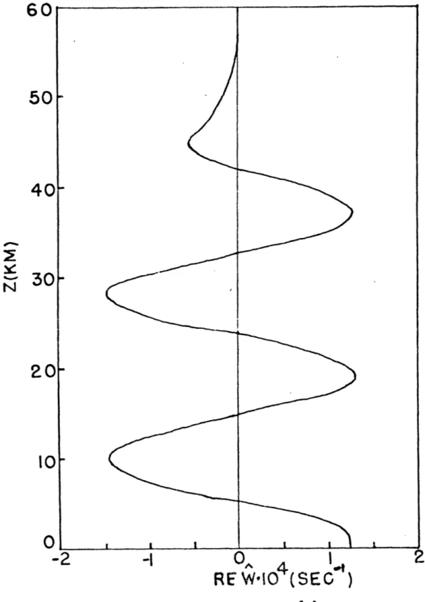
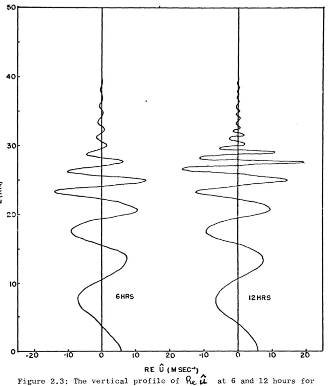
Z. . Here e. at 45 km is the lower boundary of the damping region. A critical level for the forced wave motion exists at 30 km where u0 = 55.5 m/sec. The graphs ofu at x = 0 and the term -g~ Lk W which is proportional to the
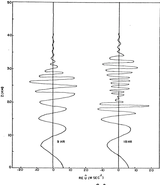
momentum flux are presented in Figs. (2.3, 2.4) at various times.
The transmission of wave energy can be followed from the form of the momentum flux with time. The region of decrease in momentum flux moves upward more slowly as it approaches the critical level in agreement with the decrease in group velocity given by simple, theory. Very little flux occurs across the critical level and the momentum flux discontinuity at the critical level is becoming
established. The small scale features in the momentum flux are the result of transient motions caused by the impulsive start of the forcing at t = 0. As time goes on the flux approaches a constant value below the critical level.
cc
6HRS 12HRS
10
20 -10 010
20RE U (MSEC-')
Figure 2.3: The vertical profile of
9
at 6 and 12 hours for wave motions propagating through a mean wind field which increaseslinearly with height. A critical level for the wave motions exists at 30 km. 'I 40
301-(
~ZZZ
201--2040
30-
20-36
9
12
10-0
I
2
3
4
5
0
1
2
3
4
5
0
1
2
3
5
RE
1/2
UW-1
(M SEC)
Figure 2.4: The distribution of the termlil$uwhich is proportional to the momentum flux, at three hour intervals from 3 to 12 hours for wave motions propagating through a mean wind field which increases linearly with height. A critical level for the wave motions exists at 30 km.
The graphs of u show the decrease of vertical wavelength as the waves propagate through the region of positive wind shear and the growth of the magnitude of the motions near the critical level. Very little motion occurs above the critical level.
Case III: Time dependent mean flow
This case has also been treated by Houghton and Jones~(1968) in a somewhat different manner. The novel feature presented here is the integration of equation (26) for the local value of
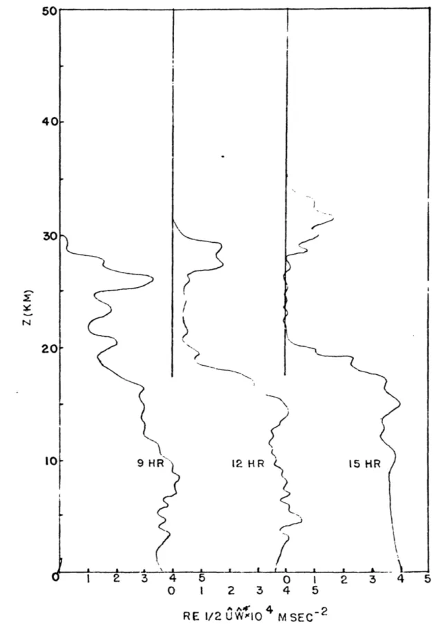
The calculation proceeds exactly as in the previous case for six hours. From six to nine hours the vertical gradient of the mean wind is increased uniformly until the critical level, originally at 30 km, is lowered to 20 km. The calculation is continued for a further nine hours. The resulting values of the momentum flux and the u component of velocity are shown in Figs. (2.5a,2.5b).
The wave motions shown in the figures can be most easily understood by considering the time dependent behavior of the local value of the intrinsic frequency C'= I - LtLk . The local
frequency
1)
is a function of z and t as is %A*(j~t
in this case. Fig. (2.6) shows the value of 'T~ for the six hours follow-ing the beginnfollow-ing of the acceleration of the mean flow. Before the acceleration of the mean flow, the waves could not penetrate the level where \A. 5 -4 SC' * The accelerationN 10 9 HR I8HR 01 -20 - 0 10 20 -10 0 10 20 RE U (M SEC
Figure 2.5a: The vertical profile of QA.', at 9 and 18 hours for the case of a time dependent mean wind.
20
10-
9 HR ' 12 HR 15 HR3
4
5
0
2
34
5
0 1 2 3 4 5 A^^J 4-2
RE 1/2 UW)I0 M SECFigure 2.5b: The vertical distribution of the termL k.A, which is proportional to the momentum flux of the waves, at 9, 12 and 18 hours for the case of a time dependent mean wind.
V\ I
-20
O
IC
4 -'
0~~-I0
(SEC~')
Figure 2.6: Time dependent behaviour of the local value of a for the case of the mean wind changing with tim±e. The straight lines give the distribution of a appropriate to a constant mean wind which increased linearly with height with a critical level at 30 and at 20 km. The curves show the behaviour of a as the mean wind changes with timefor 3 and 6 hours after the beginning of the change.
of the mean flow alters the local value of the frequency of the waves and waves now exist in the region where
LAo
)
55.5 m/sec. The waves will continue to propagate upward towards the critical levels definedby their altered frequencies. The critical levels so defined will differ depending on the value of the frequency when the acceleration of the mean flow was begun. No one critical level exists and a critical region is more correctly referred to.
The behavior of the momentum flux and the u component of wave motion shows this effect. There is a continued propagation of energy into the regions above the original critical level at 30 km. The new critical level at 20 km, for motions forced at the lower boundary, prevents propagation of energy past this level and the motions are separated into two regions.
Case IV: Shearing region.
The mean wind in this case has a shearing level as shown in Fig. (2.7a). A critical level exists where Lko = 55.5 m/sec. The
integration is done with At = 30 sec, Az corresponding to 125 m, and the amplitude of the forcing term at the lower boundary proportional
to (
I
- . ) ,&
= (1 hr) . The resulting momentum fluxand horizontal wave velocity is shown in Figs. (2.7a, 2.7b) for 12 hours.
In this case the effects of the wind shear and the critical lev-el on the wave motions are confined to a rlev-elativlev-ely small region in the vertical. The discontinuity in the momentum flux at the critical
25
20
15
N
10-
5-20 40 60 0U.
(M SEC-)
RE
1/2
UW10
4tM
SEC
2 Figure 2.7a: The vertical profile of the mean windiLoand of the momentum flux termQa4.oiZshowing the sharp decrease of the flux across the critical level where U0=55.5m/sec. after 12 hours.N
10
-0
-20
-10
0
10
20
RE U (M SEC~)
A
Figure 2.7b: The vertical profile of k*A after 12 hours for wave motions propagating through a mean wind field with a shearing region containing a critical level.