Automated tactile sensing for object recognition and localization

AUTOMATED TACTILE SENSING FOR OBJECT RECOGNITION AND LOCALIZATION

by

JOHN LEWIS SCHNEITER

B.S. Mech. Eng., University of Connecticut (1978)

M.S. Mech. Eng., Massachusetts Institute of Technology (1982)

SUBMITTED TO THE DEPARTMENT OF MECHANICAL ENGINEERING

IN PARTIAL FULFILLMENT OF THE REQUIREMENTS FOR THE DEGREE OF

DOCTOR OF SCIENCE IN MECHANICAL ENGINEERING

at the

MASSACHUSETTS INSTITUTE OF TECHNOLOGY

Q

Professor Thomas B. Sheridan Thesis Supervisor

Accepted by... ...

Professor Ain A. Sonin Chairman, Department Committee

JUL28 1986

AUTOMATED TACTILE SENSING FOR OBJECT RECOGNITION AND LOCALIZATION

by

JOHN L. SCHNEITER

Submitted to the Department of Mechanical Engineering on April 28, 1986 in partial fulfillment of the requirements for the Degree of Doctor of Science in

Mechanical Engineering

ABSTRACT

Automated manipulation systems operating in unstructured environments, such as undersea or in space, will be required to determine the identity, location and orientation of the various objects to be manipulated. Vision systems alone are inadequate for the successful completion of some of these recognition tasks, especially when performed where vision is partially or totally occluded. _{Tactile sensing is useful in such situations, and} while much progress has been made in tactile hardware develop-ment, the problem of using and planning to obtain tactile infor-mation has received insufficient attention.

This work addresses the planning problem associated with tactile exploration for object recognition and localization. Given that an object has been sensed and is one of a number of modeled objects, and given that the data obtained so far is in-sufficient for recognition and/or localization, the methods de-veloped in this work enumerate the paths along which the sensor should be directed in order to obtain further highly diagnostic tactile measurements. Three families of sensor paths are found. The first is the family of paths for which recognition and

localization is guaranteed to be complete after the measurement. The second includes paths for which such distinguishing

measurements are not guaranteed, but for which it is guaranteed that something will be learned. The third includes paths for which nothing will be learned, and thus are to be avoided.

The methods are based on a small but powerful set of ge-ometric ideas and are developed for two dimensional, planar-faced objects. _{The methods are conceptually easily generalized to}

handle general three dimensional objects, including objects with through-holes. A hardware demonstration was developed using thick "2-D" objects, and it is shown that the strategy greatly reduces the number of required measurements when compared to a random strategy. _{It is further shown that the methods degrade} gracefully with increasing measurement error.

Acknowledgements

The first half of this research was supported by the M.I.T. Sea Grant College Program (National Oceanographic and Atmospheric Administration), and the last half by the Ames Research Center, National Aeronautics and Space Agency, under Grant No. NCC 2-360.

I thank my thesis supervisor, Professor Thomas B. Sheridan, for providing me with the opportunity to grow, for providing support and encouragement, and for being a good friend.

I also like to thank my committee members, Professor Tomas Lozano-Perez of the M.I.T. Artificial Intelligence Laboratory, whose own work provided the springboard for this work, and whose

comments and interest have been very valuable, and Professor Steven Dubowsky, for his support, comments, and valuable suggestions.

I would like to thank all the members of the Man/Machine Systems Laboratory, past and present, who have made this experience stimulating and enjoyable. Special thanks go to Jugy, Jim, Max and Leon, for the many conversations, both

pro-fessional and personal, that have helped me in many ways.

A special word of thanks goes to Erik Vaaler, whose interest, support and friendship has been of great personal value.

Without my wife Andrea, I could not have gotten this far; her love, compassion and patience is a blessing.

Table of Contents Char Chap ter 1: Introduction... 1.2 A Simple Example... 1.2.1 Features... ter 2: Recognition and Representation... 2.1 Previous Work in Recognition... 2.2 Previous Work in Representation... 2.3 An Appropriate Representation and Recognition...

Scheme for Tactile Sensing

2.3.1 The Interpretation Tree... 2.3.2 Pruning the Interpretation Tree... ter 3: A Sensing Strategy Assuming Perfect ...

Measurements

3.1 Active Touch: A Sensing Strategy... 3.1.1 Optimal Paths... 3.1.2 Suboptimal Paths... 3.1.3 Unequal Distribution of Interpretations.. 3.2 Implementation... 3.2.1 Blocking Boundary Generation... 3.2.2 Path Generation... ter 4: Strategy in a Real Environment: ...

Measurement Errors

4.1 Bounds on Transform Error... 4.2 Bounds on Computed Positions and Orientations... 4.2.1 Effects of Orientation Uncertainty... 4.2.2 Effects of Translational Uncertainty... 4.2.3 Combining Uncertainties... 4.3 Implementation with Transform Error...

4.3.1 Discretization of the Multi- ...

Interpretation Image

4.3.2 Scaling and Mapping the MIT ...

onto the Grid

Chap Chap 6 10 13 17 17 21 23 24 27 32 34 39 45 49 52 53 56 61 62 65 65 68 69 71 71 72

4.3.3 Boundary Growing... 4.3.4 Developing the MII on the 4.3.5 Path Generation... 4.3.6 Simulation Results... ter 5: Hardware Demonstration System... 5.1 E2 Master/Slave Manipulator... 5.2 Tactile Sensor... 5.3 Computer and Software Structure.... 5.4 Performance... ter 6: Generalization to Three Dimensio 6.1 Strategy in 3 Dimensions... 6.2 Generating 3-D Volumes... 6.2.1 Boundary Growing... 6.2.2 Blocking Boundaries... 6.2.3 Determining Intersection

and Union Volumes

6.3 3-D Objects Using 2-D Techniques... 6.4 Computational Issues... Grid... ns 81 84 88 92 95 97 99 101 101 102 103 104 105 ... 106 . . .. . . . .. 10 8

Chapter 7: Summary, Conclusions

References... Appendices Appendix 1 Appendix Appendix Appendix and Recommendations. ...

Representation, Recognition and .

Localization Equations

Grid Equations... Sensor Design... Finding the Intersection Area ...

and its Centroid Chap Chap ... 110 ... 115 ... 120 ... 132 ... 136 ... 142

CHAPTER 1

Introduction

Automated manipulation systems operating in

unstruc-tured environments, such as undersea or in space, will be

required to determine the identity, location and orientation

of the various objects to be manipulated. It has been known

for some time that vision systems alone are inadequate for

the successful completion of some of these recognition

tasks, especially when performed where vision is partially

or totally occluded [1-4].

Tactile sensing is useful in

such situations, and while much progress has been made in

tactile hardware development [4,51-53], the problem of using

and planning to obtain tactile information has received

in-sufficient attention [2,3,5].

A few researchers in the

en-gineering community have made attempts to develop sensing

strategies [5,6] but most of the attention focused on

so-called "active touch" has originated in the psychological

community [7,8].

This work focuses on the planning problem associated

with tactile exploration for object recognition and

localization (the determination of object position and

orientation).

Given that an object has been sensed and is

one of a number of modeled objects, and given that the data

obtained so far is insufficient for recognition and/or

localization, the methods developed in this work enumerate

the paths along which the sensor should be directed in order

to obtain further highly diagnostic tactile measurements.

Three families of sensor paths are found. The first is the

family of paths for which recognition and localization is

guaranteed to be complete after the measurement. The second

includes paths for which such distinguishing measurements

are not guaranteed, but for which it is guaranteed that

something will be learned.

The third family is made up of

paths for which nothing will be learned, and thus such paths

are to be avoided.

The recognition of an object and the determination of

its position and orientation in space is a task domain that

may be categorized into two classes. The first may be

de-scribed as the domain of passive information gathering, in

the sense that an object is presented to some suitable

tac-tile sensor and as much information is extracted from the

object is dropped onto a tactile array and the object's

"footprint" is analyzed [50].

Given that most objects of

interest have a finite number of stable poses on the plane

and that the footprint is often unique for each pose of each

object, an assessment may be made of an object's identity,

location and orientation. These procedures are open-loop in

the sense that feature information is extracted from the

sensor "snapshot" and no attempt is made to actively pursue

the gathering of more information. Such procedures are not

addressed in this work because they are primarily useful

only in reasonably structured environments.

The open-loop procedures contrast with the other class

of recognition and localization problems in which

infor-mation is actively sought by a tactile system. An example

of the latter is where some suitably instrumented

manipulator scans the surface of an object of interest,

ob-tains tactile data, and performs additional planned data

gathering based upon an analysis of the previously obtained

data. The salient description of this (serial) process is:

1. obtain data

2. analyze the data

3. plan where to direct the sensor to obtain more data,

if necessary

4. repeat as appropriate.

A good tactile scanning strategy should provide an

evolving plan or schedule of sensor moves for a system to

make in order to efficiently obtain tactile data of high

diagnosticity. Such a plan bases the next sensor move on

what has been learned from all previous measurements,

including the last. As will become evident in the remainder

of this thesis, a small but powerful set of geometric ideas

is central to the development of such a strategy. Before

proceeding directly to the development of these ideas,

how-ever, we will first explore the issues by way of a simple

example, and then delve more deeply into the nature of

tac-tile information, the notion of features, object

representa-tion and recognirepresenta-tion, and the issues of real-world

applications and hardware requirements.

The thesis is therefore structured as follows: The re-mainder of-this chapter presents a simple example to

motivate the problem and introduce some of the issues. Chapter Two provides a review of tactile work to date and explores some of the common object representation and recog-nition schemes (most of which were developed primarily for vision work) with critical attention paid to their

suitability in the tactile domain. It is here that a repre-sentation and recognition scheme is selected and explained. Chapter Three develops a tactile scanning strategy in a two dimensional environment, assuming perfect touch sensing measurements. In Chapter Four the effects of measurement error are assessed in terms of their impact on system per-formance and software implementation. The generalization of the work to include three dimensional objects is discussed in Chapter Five.

A hardware demonstration system was developed that in-corporated the ideas presented in this thesis. A descrip-tion of the system, including the manipulator arm and tac-tile sensor, and an assessment of performance issues is pro-vided in Chapter Six.

Conclusions and recommendations for further work are found in Chapter Seven.

1.2 A Simple Example

Let us assume that there is a stationary 2-dimensional object in the environment that we can obtain contact

measurements from, and let us further assume that we know it is one of two objects (see figure 1.1) we are familiar with.

Figure 1.1. Two Simple Object Models

Our job is to determine which object model represents the real object and what the transformation between model and world coordinates is by reaching out and exploring the real object using touch. We are immediately faced with the following question: What is the nature of our measurements? If the objects are of different stiffness, we have only to grope until we contact the object and then simply press against it and monitor the force/displacement behavior to recognize the object. We would still be required to explore the object's surface in some (presumably) intelligent way to determine orientation. If the objects are stiff and made of the same material, then we are forced to rely exclusively on tactile surface exploration for both recognition and

localization.

It is evident that, except possibly for the case in

which the object is smaller than some sensor array (in which

case the sensor might obtain a "snapshot"), tactile

exploration of the object's surface will in general be

necessary. With a contact-point sensor we have to obtain

surface information from multiple contacts between the

sen-sor and the object.

If we have an array of sensitive

elements, we can obtain local patches of surface data from

which we might calculate surface properties such as the

local surface normal and surface curvature. (This is nothing

more than a parallel implementation of a single point

con-tact sensor that provides the data in a more serial manner).

In this way we can

of the object with

Let us assume

contact points and

We have to map the

equivalently, fit

unique the job is

be multiple possib

cases the data is

objects,

build up a sparse spatial tactile image

a series of contacts.

,

then, that tactile data is comprised of

measured or derived surface properties.

data onto the object models or,

the models to the data.

If the mapping is

complete. In general, however, there will

le interpretations of the data.

In such

insufficient to distinguish between the

or if it is sufficient to distinguish, we may still

be unable to determine position and/or orientation. Figure

1.2 shows an example of contact data consisting of contact

position (at the base of the arrows) and measured surface

normal (represented by the arrows) which do not distinguish

between the objects. The same data fits each object in only one way equally well.

A A

B B

C C

Figure 1.2. Non-Distinguishing Data

Figure 1.3 depicts the case where the data distin-guishes between the objects but we are left with multiple orientations of the object.

A A

C B C B

C C

Figure 1.3. Non-Distinguishing Data

We must now determine what measurements to make next. This raises another question: Under what constraints do we operate? We have to know the relative costs of movements, measurements and time in order to respond to this question. If the cost of information processing (processing time, noise smoothing, etc.) is higher than the relative cost of

moving the sensor (travel time, risky movements in an

unknown environment, etc.) then it is appropriate to seek

distinguishing features wherever they might be.

If,

conver-sely, information processing is relatively inexpensive and

long range movements expensive, it might be more appropriate

to explore a local surface. This can be very wasteful,

how-ever.

For example, in Figure 1.2, local exploration of the

surfaces at either B or C will yield no useful information.

This lends support to the assertion that in general, a

pur-poseful, active tactile sensing strategy should direct the

sensor to the most distinguishing features available.

As an aside, we make the intuitive observation that in

general, the more complex the objects, the more features

there are available, hence the more likely a random strategy

is to be powerful and successful.

It is when the objects in

a set are similar that we find we need a good strategy.

Maximally different objects can possibly be distinguished on

the basis of local surface analysis, whereas minimally

dif-ferent objects are more likely to require global or

struc-tural analysis.

1.2.1 Features

We have used the term feature without rigorously

defin-ing it.

One definition (from Webster's) that is appropriate

in our context is that a feature is a "specially prominent

characteristic".

For our purposes, the characteristic must

be measurable or derivable from measurements. We therefore

assume a feature to be a measurement (or a quantity derived

from a measurement) that provides us with information. We

notice immediately that this is dependent on the object set

under consideration. For example, in Figure 1.4 the object

set is comprised of objects A and B. Surface normal

measurements from the triangular structure on object B,

along with normal measurements from other parts of the

ob-ject, inform us that the object cannot be object A.

Figure 1.4.

Object Set for which surface

normals distinguish.

However, in figure 1.5, simply measuring surface

nor-mals is insufficient to discriminate between objects.

Figure 1.5.

Object set for which surface

normals and associated contact

positions distinguish.

We see, then, that discriminating features depends upon

the composition of the object set.

If a scanning strategy

is to be useful, i-t should automatically perform feature

se-lection from among the object models and should require no

more of us than correct models. We should not be required

to select features a-priori (assuming that we are

sophis-ticated and patient enough to do so) and we should be able

to add objects to the object set and delete them at will.

If we are to automate active touch, we must have some

way of representing objects in a computer in a way that is

natural, efficient, and allows for fast processing. While

these may be subjective notions, it is clear that techniques

which require more computer memory than is reasonably

avail-able or routines that take days to run on standard, powerful

equipment are to be avoided. The next chapter reviews many

of the standard representation and recognition schemes in

view of tactile sensing requirements, and describes the one

16

CHAPTER 2

Recognition and Representation

Our ultimate objective is to produce a strategy for

ob-taining tactile data, but we must first discuss how we plan

to represent objects and how we can recognize them using a

computer. The purpose of this chapter, then, is to briefly

review the previous work in tactile recognition and comment

on why the various methods have proven unsatisfactory, to

discuss various representation schemes that have been

devel-oped (historically, primarily for vision work), and to

de-scribe the representation and recognition methods chosen for

this work. The review is rather brief because there are

al-ready a few very thorough reviews in the literature.

The

interested reader is referred to two reviews by Harmon

[1,4], a review by Gaston and Lozano-Perez [35], and a

review by Grimson and Lozano-Perez [27].

2.1

Previous Work in Recognition

There are two major alternative approaches to

recog-nition in the tactile sensing domain: pattern recogrecog-nition

and description-building and matching. The basic notion in

classical pattern recognition is the notion of a feature

vector [9-13].

The available data is processed and a vector

is created to represent the results of the processing. For

example, the pressure pattern on a tactile array can be

of inertia of the pattern, and these moments can be used as

the elements of a vector (the feature vector).

The

recog-nition process is performed by comparing the feature vector

with previously computed vectors for different objects.

Recognition is typically assumed complete when the feature

vector matches a model vector fairly closely. The matching

criterion is typically the Euclidean distance between the

vectors.

If the feature vector does not match any of the

model vectors closely enough, then typically another feature

is extracted from the data and the process is repeated.

Most of the previous work in tactile recognition using

these ideas used either pressure patterns from two

dimen-sional objects on sensor arrays [50,54] or the joint angles

of the fingers that grasp the object [55,56] as the data.

Some work combined the two approaches [57].

There are two

major objections to these approaches.

The first is that we

can not expect a two-dimensional sensor array to provide

enough data for recognition of complex three-dimensional

shapes. Furthermore, the range of possible contact patterns

that might arise in practice can be quite large and

precom-putation of them would be impractical.

The second objection

is that the range of possible graspings of an object can

also be quite large, which effectively prevents

precom-putation of all possible finger positions and joint angles.

In summary, tactile recognition based on classical pattern

recognition is limited to simple objects, primarily because

of the great cost in precomputing feature vectors for more

complex objects. Another point, expressed in [27], is that

the methods are limited because they do not exploit the rich

geometric data available from complete object models.

A relatively recent branch of pattern recognition

theory is called syntactic pattern recognition and is based

on the observation that object shapes can in some sense be

associated with an object "grammar" or rules of structure

[10].

It has enjoyed some success in two dimensional vision

work but has been relatively unsuccessful in 3-D recognition

because the appropriate grammars are extremely difficult to

devise for even fairly simple 3-D objects.

In description-based recognition methods, a partial

description of an object is built up from sensor data and an

attempt is made to-match the partial description to an

ob-ject model.

Approaches have included building the

descrip-tion using multiple contacts of a pressure sensitive array

[58] or from the displacement of the elements in a sensor

comprised of long needles [59,60].

Although the

description-based approach may be more general than the

pat-tern recognition approach in its ability to handle complex

3-D shapes, it suffers from the requirement that a great

deal of data must be obtained. Furthermore, there are few

methods for actually matching the data to object models, and

the methods are computationally expensive.

Most current researchers in the tactile field

implicitly (and I feel correctly) assume that tactile

sen-sors will be integral components of manipulation systems,

20

and will be required to impart forces to objects as well as

obtain surface information from them. This will require

some moderate stiffness of the sensors, so we can not assume

that we can ever obtain a great deal of dense surface data

from an object with a single measurement, since that would

require a very soft, easily deformable sensor that can be

draped over a large part of an object. Tactile sensors

useful in manipulation systems will, by their very nature,

provide fairly sparse surface data. While we might obtain

dense surface data from an object by an exhaustive tactile

scan, it is clearly inefficient to do so, because intrinsic

geometric constraints [27] associated with any object can be

exploited to yield recognition and localization with only a

few tactile measurements.

For this reason we assert that classical pattern

recog-nition and description-based techniques that require dense

surface data are of limited utility to the tactile problem.

While the essential goal of of these methods, that of

recog-nizing and localizing an object based on sensor

measurements, is essentially what we wish to accomplish, the

methods available are inappropriate in our problem context.

21

2.2

Previous Work in Representation

Automated recognition, or the matching of sensor

data to object models, requires some representation

struc-ture that can be described mathematically or algorithmically

and programmed into a computer. We need some way of

rep-resenting objects that is natural and appropriate to the

data we will obtain. For the case of tactile recognition,

we require a surface-based representation that allows for

fast, efficient processing of sparse data. Representation

structures such as solid modelling (28], oct-trees [30],

generalized cylinders [31,32], tables of invariant moments

[22,23], fourier descriptors [29,38], and such are basically

volumetric representations and generally require extensive,

dense collections of data, and are therefore not

particu-larly acceptable for tactile work.

Surface-based representation schemes have been

de-veloped for use in CAD/CAM systems [33], for object

recog-nition using laser range data

[19,27], and for some vision

work [34].

These typically belong to one of two categories.

In the first category, object surfaces are modeled by

patches of parametric surfaces such as quadric polynomials

[19-21], bicubic spline patches

[33], Bezier patches and

cartesian tensor product patches [33].

These patches are

typically selected by the analyst and used to build up a

model of an object. An objection to the use of such methods

matching of data to model surfaces is complicated,

es-pecially if there is sensor error.

The second category of surface-based representation

methods is in some sense a subset of the first, but has

dis-tinct features that make it important in its own right.

This method segments an object's surface into planar facets

[17-21,34], where a least squares analysis is made of the

error between the modeled planar facet and the true object

surface. During the modeling phase, planar model faces are

"grown" until the error reaches some prescribed threshold,

whereupon a new facet is started (There will be, admittedly,

a large number of faces in regions of moderate to high

cur-vature using this technique, with a concurrent increase in

model complexity).

An important aspect of this

representa-tion is that, during the recognirepresenta-tion phase of contemplating

where data might have come from, there is a bounded finite

number of interpretations of the data, i.e., of assignments

of data to faces.

This still requires fairly dense sensor

data, but it considerably simplifies the model matching

problem that is so severe in the general parametric surface

representation.

2.3

An Appropriate Representation and Recognition

Scheme for Tactile Sensing

The tactile sensing work of [27,35] employs a

represen-tation and recognition structure that is quite appropriate

in light of the preceding discussion, and is the one chosen

for this work. It uses a surface description that segments

objects into planar patches and assumes that tactile

measurements are comprised of the single point of contact of

the sensor with a face of an object and the surface normal

of the face at that point.

Object representation is embodied in tables of face

vertices, normals, and tables of constraints between

dis-tances, normals and directions between all pairs of faces

for each object. The set of possible assignments of data to

model faces can be structured as an Interpretation Tree

[27], which is quickly and efficiently pruned by first

exploiting the constraints and then performing model checks

on remaining branches to determine what possible positions

and orientations of which objects are consistent with the

data. The method is quite fast and degrades gracefully with

increasing measurement error. It is limited to planar

ob-jects and makes no use of derived properties of surfaces

such as curvature, although it is easily generalized to

include such information.

(Such information is useful only

if.it can be reliably obtained. Since curvature is

essen-tially a second derivative, it is quite sensitive to

measurement error, and hence may not be useful if a

numerical value is required.

It may be possible, however,

to reliably measure and use the sign of the curvature.)

A demonstration of the method assuming fairly complex

three-dimensional objects, as well as a detailed analysis of

the process, is given in [27].

A presentation of the

impor-tant equations in modified form is given in Appendix 1. We

motivate and discuss the salient points in what follows.

2.3.1

The Interpretation Tree

We assume that the sensed object is one of a number of

modeled, possibly non-convex polyhedra.

In the general

case, the object may have up to six degrees of positional

freedom in the global coordinate system. As previously

men-tioned, the sensor is capable of conveying the contact

position and object surface normal in the global system.

The goal of the system is to use the measurements to

deter-mine the identity, positions and orientations of objects

that are consistent with the data. If there are no

al-lowable positions and orientations of a candidate object

that are consistent with the data, we can discard the object

as a contender.

Thus, we can solve the recognition process

by doing localization, and we therefore concentrate on that

problem.

models, we proceed as follows:

-

Generate Feasible Interpretations:

There are

only a few credible mappings of data to faces based upon

local constraints. Mappings of data to faces that violate

these constraints are excluded from further attention.

-

Model Test:

Only a few of the remaining

in-terpretations are actually consistent with the models in the

sense that we can find a transformation from model

coor-dinates to global (or data) coorcoor-dinates.

An interpretation

is allowable if, when the transformation is applied to the

model, the data lie on the appropriate finite faces, and not

simply on the infinite surfaces defined by the face

equations.

We generate feasible interpretations of the data as

follows.

When we obtain our first sensed point, we can

as-sign it to any of the faces of any objects if we have access

to no other information. This is graphically depicted on

what is called the Interpretation Tree (IT) [27].

26

0e

Z

Figure 2.1 Interpretation Tree (from [27]).

At each level we have another sensed point, and if we do no analysis, we can assign that point to any of the ob-ject's faces. Each branch of the IT represents the in-terpretation that the sensed point at that level belongs to a particular face. There is a total of s levels in the tree, where s = number of sensed points. Since two or more points might possibly lie on the same face, each node of IT.

J has e. branches. This essentially represents the search

J

space for feasible interpretations of the data. If we can perform some analysis to prune away entire subtrees, we can reduce the number of computationally expensive model tests to perform.

The number of possible interpretations of the sensed points is [27]

m

(n.

S

i=1

where m = number of known objects n. = number of faces on object i s = number of data points.

This can become quite large, which implies that it is

not feasible to perform a model check on every conceivable

interpretation. Note that the number of possible

in-terpretations (possible combinations of assignments of data

to faces) increases exponentially with the number of sensed

points, whereas the set of feasible interpretations is

reduced. We exploit local geometric constraints to exclude

large sets of possible interpretations (subtrees) and

gener-ate the much smaller set of feasible ones.

2.3.2

Pruning the Interpretation Tree

We can make use of geometric constraints to prune the

IT without having-

to perform model checks. Although there

are many constraints that can be exploited, the following

three are quite powerful [27].

The reader is referred to

Appendix 1 for a detailed explanation of the constraints and

of the pruning process.

1. Distance Constraint.

If we are to

con-template assigning sensed point 1 to face i, and sensed

point 2 to face

j,

then the distance between points I and 2

must be between the minimum and maximum distances between

any points on faces i and j. See figure 2.2.

2. Angle Constraint. The angular relationship

between sensed normals must be the same as that between the

assigned faces in an interpretation. If we allow for

an-gular error on the sensed normals, the range of possible

angles between the sensed normals must include the angle

be-tween the normals of the assigned model faces paired with

them in an interpretation.

3. Direction Constraint.

The range of values

of the component of the vector from sensed point 1 to sensed

point 2 in the direction of the measured normal at point 1

must intersect the range of components of all possible

vec-tors from face i to face j in the direction of the modeled

normal of face i, where faces i and j are paired with sensed

points 1 and 2 in the interpretation. The same must be true

in the other direction, from point 2 to 1 and face

j

to i.

Note that, in general, the ranges are different in the

dif-ferent directions; this test is not symmetric.

The application of the constraints has the effect of

pruning entire subtrees of the IT, thereby vastly reducing

the required number of model checks.

In general, a few

in-terpretations will survive constraint pruning and model

checking. This means that there is not enough information

in the data to decide on a single interpretation (presuming

the object(s) is (are) not biaxially symmetric, in which

case multiple interpretations are equally correct.)

We perform model checks on the surviving

in-terpretations to insure that the data actually fits on the

finite model faces, and not simply on the infinite faces

de-scribed by the face equations.

For each feasible

in-terpretation we calculate the the angle e which rotates

the model, and the translation V

which translates the model

so that the model matches the data. The transformation

equation applied to each vertex Vm of the model to produce

V in the global system is

V = R V + V

-g

-m

-0

or

0

1

1

V]

our 2 D case,

R

=

[

)

-sine

and

0=

[

tr

sin8 cos9)Yt

We find e by computing the difference between the

sensed normal direction and the normal direction of the face

assigned to that sensed normal in the interpretation.

If we

allow for measurement error, we calculate e by averaging

the computed differences for all sensed normals.

(Determining orientation in three dimensions is considerably

more complex. See Grimson and Lozano-Perez [27] for

devel-opment.)

We use position and normal measurements to determine

the translation component of the transformation. The

devel-opment of the expression relating these measurements to V

appears in Appendix 1. The relation is

[k.(Rni x Rnk)]VO =

(Rng.V

(R-k'

gk-dk)(k

x Rn ).

Again, if we allow for measurement error, we compute V0

for all data pairs and average the results.

We now have to contemplate obtaining another

measurement, and it is here that the notion of a strategy

becomes important. We could simply choose another sensing

direction at random, which might leave us with as many

in-terpretations as we now have, or we can try to choose a path

31

which gives us a measurement with highest information

con-tent.

We focus on 2-D objects in order to more clearly

motivate and more simply develop a sensing strategy. The 2-D

representation and recognition case is contained in the more

general 3-D case with no significant change in the process

[35].

The generalization to three dimensions of the ideas

32

CHAPTER 3 A Sensing Strategy Assuming Perfect Measurements

This chapter addresses the planning problem associated with active touch, i.e., determining some "intelligent" schedule of sensor moves based upon a knowledge of modeled objects and the tactile information obtained thus far. Spe-cifically, given that an object is in the environment and is one of a number of modeled objects, the objective is to

determine the identity, location and orientation of the ob-ject, using tactile signals only, by selecting the best path along which to direct the sensor for the next measurement. The best path at any stage in the process is the path for which the ratio of the cost in taking the measurement with the expected gain in information is minimum. We woud.-typically choose paths for which recognition and

localization would be complete after the next measurement (a "distinguishing measurement"). If constraints such as

maneuverability or time are important, however, a system might choose to take somewhat less diagnostic measurements, but under no circumstances should it take measurements of zero diagnosticity. Purposeful, directed tactile

exploration should not include making moves when it is cer-tain that nothing will be learned.

Therefore, the "strategy engine" for a system should generate three generic families of sensor moves for use by a higher level strategist, one that itself bases candidate

moves on the strategy engine's output, knowledge of the physical arm configuration, torque limits, task specifica-tions, etc.[61j. The first of these is the family of moves that guarantee recognition and localization with the next measurement, if such moves exist. The second family

pro-vides suboptimal moves in the sense that there is no guaran-tee of a distinguishing measurement, but at least something will have been learned. It will be shown that, assuming perfect measurements, this family of paths is not null

ex-cept in the case of a single, biaxially symmet.ric object, where it is meaningless to talk about absolute orientation anyway. Finally,~the third family contains paths that will provide absolutely no new information after the next

measurement is made (and thus are to be avoided). It will be shown that this family is also not null if perfect

sers-ing is assumed.

If one intentionally probes a specific surface in order to distinguish between objects (which implies that

some minimal amount of information has already been

obtained), one must have an idea of the positions and orien-tations for all the interpreorien-tations in order to decide upon a path. Therefore, the problem of object recognition and

localization using a strategy contains the problem of ob-ject localization when the obob-ject is known. Hence, to fix ideas and motivate the method, we will solve the following simple problem: What are the conditions for generating the three families of paths, and what are these paths, for the

case of localization of a single, known, planar 2-D object with perfect measurements of tactile contact positions and measured surface normals?

3.1 ACTIVE TOUCH: A SENSING STRATEGY

When an automated tactile recognition system begins its search, there is no more information available than perhaps that there is an object in the environment. Any strategy would simply be forced to implement some sort of blind search. Once contact has been made the situation is dif-ferent, although the first measurement may not tell us much. For instance, if we are dealing with planar objects and ob-tain a point and normal at a face of an object of n faces, there are n possible orientations with a one-parameter fam-ily of translations for each orientation. Any other

measurements m such that In..n j1, where n -is the -th nor-mal measurement, lead to a similar result, although perhaps

the number of orientations and the allowable ranges of translations may be reduced. The only reliable way to

constrain the interpretations is to obtain at least two

measurements with normals obeying fn|*.2I|l, because then the translational degrees of freedom disappear.

Some methods for selecting a second measurement point might include approaching the object from a random direc-tion, or sliding along the object, or, preferably, moving to outside the envelope of translations and approaching the

ob-ject in a direction orthogonal to the first measured normal, along a ray that intersects faces for every interpretation as close to orthogonally as possible, as shown in figure

3.1.

Figure 3.1 Obtaining a constraining measurement.

Once we have constrained the object we are left with some finite number of interpretations of the data, as shown

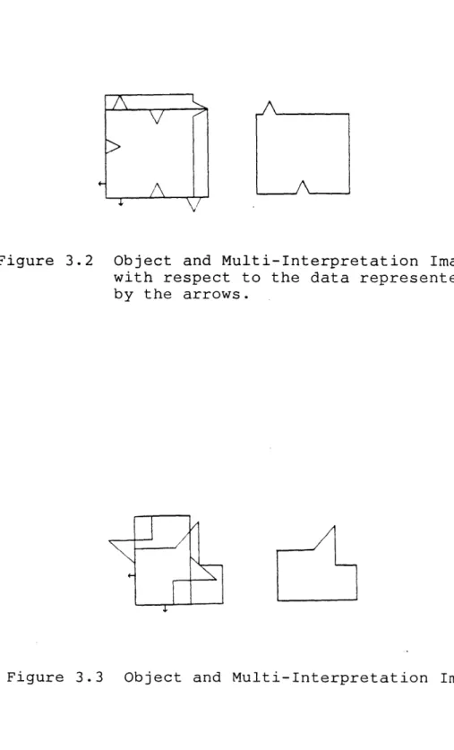
in figures 3.2 and 3.3. The composite image resulting from overlaying the interpretations will be called the

Multi-Interpretation Image (MII).

At this point it is appropriate to introduce

definitions of the entities we shall be using for strategic path generation. Denote the enclosed area (volume in 3-D) of interpretation n by A We will treat all areas (or volumes) as infinite sets on which we can perform the union and intersection set operations. See figure 3.2 for visual support of the definitions.

Figure 3.2 Object and Multi-Interpretation Image with respect to the data represented by the arrows .

Figure 3.3 Object and Multi-Interpretation Image.

V_

denoted by Ai and is bounded by an Interpretation Boundary.

Definition 2: The area AI such that

A₁ = A I A₂fn _{... fAn}

is the Intersection Area of the interpretations with respect to the data. The boundary containing A is called the In-tersection Boundary. In two dimensions, it is the boundary traced out by starting at a data site and travelling along an Interpretation Boundary in a counter-clockwise direction, always choosing the left-most path at any fork.

Definition 3: The area AU such that

AU _{= AIUA}

2 U...UAn

is the Union Area of the interpretations with respect to the data. The boundary containing AU is called the Union Bound-ary. It is obtained in 2-D in precisely the same way as for the intersection boundary except that the right-most path at any fork is chosen.

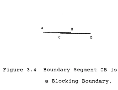
Definition 4: Any boundary or section of boundary of the composite multi-interpretation image that is common to more than one interpretation is called an Overlapping or Blocking Boundary. For example, in figure 3.4, interpretation bound-ary AB overlaps CD. The blocking boundary for this

A _B

C D

Figure 3.4 Boundary Segment CB is a Blocking Boundary.

A blocking boundary has a Degree or Strength associated with it that is determined by the number of interpretation boundaries that share it. A blocking boundary is of degree n-1 when at least n interpretation boundaries are common to

it. In the example above, blocking boundary CB is of -degree 1. For reasons that will become clear later, this

definition allows us to view a high degree blocking boundary as a lower degree boundary. For example, a blocking bound-ary of degree 2 (at least 3 boundbound-ary segments overlap) can be viewed as a blocking boundary of degree 1 because at

least 2 boundaries overlap. In general, then, any higher degree blocking boundary can (and will) be viewed as any

lower degree blocking boundary when necessary.

With these definitions we are now in a position to introduce some observations that lead to two basic theorems in strategic path generation.

3.1.1 OPTIMAL PATHS

Optimal paths are those which are guaranteed to lead to a distinguishing measurement. In order to develop a method

for finding them, an assumption and a series of observations are made regarding the nature of the measurements.

Assumption: Although we speak of the normal to a surface at a point, any device measuring a surface normal samples an area of finite size. Indeed, the surface normal is

un-defined at an edge or a vertex. We will therefore say that the distance and normal measurements are obtained from a data patch or site, and this patch is of finite length. (In 3-D, it is of some finite area.)

The following observations 1-3 are considered self-evident and are stated without proof (refer to figures 3.2 and 3.3). _{They are useful for automating the determination}

of intersection, union and blocking boundaries for 2-D planar objects. _{They are true simply because all data} points are common to the interpretations.

Observation 1: Given the multi-interpretation image arrived at from the constraining data, each data site is a segment of the intersection boundary.

40

data site is a segment of the union boundary.

Observation 3: Given that data sites are finite and non-zero, data sites always lie on finite blocking boundary seg-ments of degree n-1, where n is the number of

in-terpretations.

Observation 4: There will always be at least one finite, non-empty intersection area in the multi-interpretation image.

Proof: Part 1: Finite - The intersection area is obtained from the intersection of n finite interpretation areas. The intersection of n finite areas is less than or equal to the smallest of the areas, which will always be finite.

Therefore, the intersection area is finite, and it follows that the intersection boundary is closed.

Part 2: Non-Zero - From Observation 1, the data site is a part of the intersection boundary. Assume the

in-tersection area is zero. Then either the area of at least one of the interpretations is zero, or at least one inter-section area does not have a common overlap with the others. But we know that the areas of the interpretations are all non-zero, and there is at least one finite data patch (from

the assumption) common to all the interpretations, which implies overlap to some extent; the intersection area must be non-zero.

//

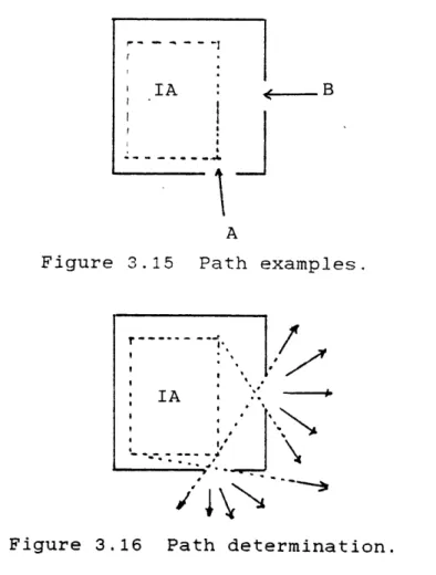
Observations 1-4 motivate and support theorems 1 and 2, which form the basis of the sensing strategy. First, let us view an example. Figure 3.5 shows the object and

in-terpretations from figure 3.2 along with members of the fam-ily of paths that are guaranteed to produce data unique to only one interpretation. Notice that for each path, there are three distinct intersection positions and/or surface normal orientations at the intersections of the paths with each of the three interpretations. In this case, each of the paths is guaranteed to produce a distinguishing

measurement.

Figure 3.5 Paths for distinguishing measurements.

Theorem 1 describes when such families of paths are available and what distinguishes them from other paths.

Theorem 1: Assuming no measurement error, any path that originates outside the Union Boundary and terminates inside the Intersection Area without passing through a Blocking Boundary is certain to provide a distinguishing measurement.

Proof: There can be no boundaries outside of the union boundary by definition. Likewise, there can be no bound-aries within the intersection boundary. Any ray that passes

from outside the union boundary to inside the intersection boundary necessarily passes from outside to inside the area of each and every interpretation. In order to do this it must cross the boundary of each and every interpretation at

least once. If, furthermore, the path does not cross a blocking boundary, then it crosses the boundary of each and every interpretation uniyuel at least once. Therefore, since one of the interpretations is the "true" one, if the sensor is directed along such a path, it is guaranteed to touch the boundary corresponding to the true interpretation and report a unique measurement belonging only to that in-terpretation.

//

Theorem 1 implies that if a certain condition is met, namely that the blocking boundary is not closed, then at least one family of paths exists that will provide recog-nition and localization with the next measurement. It says nothing about when one can expect the the blocking boundary to be open. Indeed, the problem of determining whether the

43

blocking boundary is open is a very difficult one that I suspect has no analytic solution. It appears that a detailed geometric analysis must be performed for every situation, after every measurement, in order to derive the nature of the blocking boundary.

Theorem 1 also says nothing about the nature of any paths that might be found. In the system developed,

straight-line paths are sought. Straight-line paths are not guaranteed, however, and candidate paths can be curved in some situations. Finding a path in such situations is es-sentially a maze-running problem where the blocking bound-aries act as maze walls. Automating the development of such paths is beyond the scope of this work.

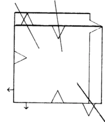
Figures 3.6 and 3.7 show the results of using the theorem in a software system that performs the geometric analysis

necessary for path generation. Each figure shows a known ob-ject along with the multi-interpretation image with

highlighted blocking boundaries. Note path examples for which distinguishing measurements are guaranteed. Each of these cases takes on the order of 10 seconds to run on a PDP11/34.

Figure 3.6 Highlighted Blocking Boundaries

Figure 3.7 Highlighted Blocking Boundaries with distinguishing paths.

We have assumed nothing about what a single object's shape must be, other than tacitly assuming closed boundaries and finite, non-zero area. Indeed, the theorem is equally valid in the case of multiple objects, where there might be multiple interpretations of different objects with respect

to the data. Here the full power and utility of the method

become apparent. For example, the difficult problem of dis-tinguishing between two very similar objects is handled

quite routinely and correctly. As an example, consider the similar objects A and B in figure 3.8 along with the multi-interpretation image associated with the constraining data shown.

A

Figure 3.8 The discrimination of two similar objects.

The appropriate family of paths is easily found.

3.1.2 SUB-OPTIMAL PATHS

Let us now focus on a different problem. There may be situations in which an optimal path is unreachable or un-desirable, or it is determined that the blocking boundary is closed. In any event, we may be willing to settle for a measurement that is more or less likely to provide recog-nition and localization in lieu of one that is certain to. The problem then becomes one of determining such paths and providing some measure of how likely they are to provide distinguishing measurements. Theorem 2 is concerned with this.

Theorem 2: Assuming that each of the interpretations in the multi-interpretation image is equally likely, any path originating outside the Union Boundary and terminating

side the Intersection Area that passes through each in-terpretation boundary once and through a single Blocking Boundary of degree m will, with probability (n-m-1)/n, pro-vide a distinguishing measurement, where n is the number of

interpretations.

Proof: Consider a path penetrating n boundaries, one from each of the interpretations, m+1 of which overlap.

Then there are n-(m+l) distinct, distinguishable boundaries from which. to obtain distinct data. Now, since we are given equal likelihood of the interpretations, the chances of ob-taining the "true" data from any chosen one of the n bound-aries is simply 1/n. The chances of obtaining the "true" data from any of the non-overlapping boundaries is therefore equal to the number of such boundaries divided by n, or

n-(m+1) n

This theorem states that if a path does cross a single blocking boundary, the chances are reduced that a fully dis-tinguishing measurement will be made. Equivalently, the chance of being left with m+1 interpretations after the measurement is (m+1)/n. This has some interesting conse-quences. The first is that, since any data site is on a blocking boundary of degree n-1, any path near the site that

passes through the blocking boundary will generate a

measurement such that the chance of being left with (n-l)+l

= n interpretations is ((n-1)+1)/n = 1. In other words, no-thing will be learned. The theorem essentially advises us to avoid taking measurements near data sites. The second consequence of the theorem is that we can now trade off movements sure to produce distinguishing data with perhaps more desirable moves less certain to produce such data.

Such moves might be more desirable because of geometric, mobility, or time constraints, etc.

A third consequence of the theorem is that we now have a way of dealing with the case of a low degree closed

block-ing boundary. It should be evident that, except for the case of a single symmetric object, there can never be a

closed blocking boundary of degree n-1 everywhere, where n =

number of interpretations. The blocking boundaries at the data sites will be of degree n-1 and extend for some length, but at other sites the boundaries will be of some lower de-gree. This means that we have only to shift our attention

to blocking boundaries of higher degree until the single closed blocking boundary "opens up". In other words, the path-finding algorithm is applied to the

multi-interpretation image as before, but paths are sought that do not intersect strength 2 blocking boundaries. At this point the path-finding routine will generate families of straight paths (if possible) just as before, only now distinguishing data is not guaranteed because candidate paths will pass

through degree 1 blocking boundaries. We will, however, have obtained the best paths available in the sense that the chance of recognition and localization is as high as pos-sible. As an example, consider figures 3.9 and 3.10. Here we have a situation in which the degree 1 blocking boundary

is closed. By simply shifting our attention to degree 2 boundaries we can find a family of paths that, while not guaranteeing recognition and localization, gives us the hig-hest probability of such (0.5 in this case).

Figure 3.9 Degree 1 Blocking Boundary is closed.

A

Figure 3.10 Degree 2 blocking boundary is open.

Note in figure 3.10 that the path intersects a single blocking boundary (shown in figure 3.9). If the path were to pass through Face A, which is also a blocking boundary,

49

there would be no chance of making a distinguishing

measurement. We know a-priori that there would be two in-terpretations remaining after taking the measurement.

An uniform, discrete distribution of the

in-terpretations is assumed in the statement of Theorem 2.

Clearly, if the physics of the problem is such that some ob-jects or orientations are more likely than others, then some interpretations will be more likely than others. If this is the case, the more likely interpretations should be weighted more heavily in the analysis. _{This is discussed in the next} section.

3.1.3 Unequal distribution of Interpretations

Theorem 2 assumes an equal, discrete distribution of the interpretations and states the probability of obtaining a distinguishing measurement if the sensor is directed along a path that passes through a single blocking boundary.

There are certain situations in which the physics of the problem imply that some interpretations are more likely than others, however. For instance, consider an object resting on a plane. _{Some poses of the object are more stable in the} presence of disturbances than others, and if the object is randomly thrown onto the plane, one would expect to observe the more stable poses more often than the less stable poses. It may also be that some faces are more likely to be sensed than others (randomly oriented object and random sense

directions), which also affects the probability of occur-rence of the various interpretations.

Under such circumstances it is appropria'te to assign unequal probabilities to the various feasible

in-terpretations one might obtain. This is a more general case and includes the uniform case as a subset.

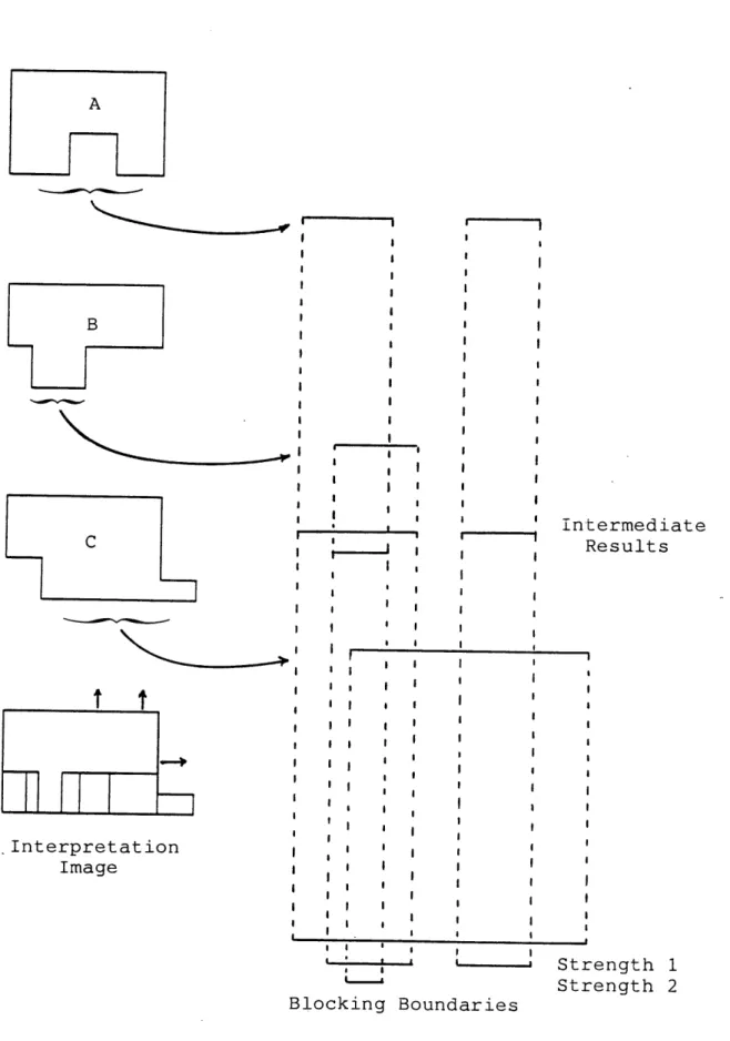
We treat the problem by weighting boundaries associated with more likely interpretations more heavily than bound-aries associated with less likely ones, and by slightly

changing the definition of blocking boundary strength. Con-sider figure 3.11, which shows a fragment of a

multi-interpretation image (MII) through which we contemplate directing the sensor. _{Each boundary segment is from a} dif-ferent feasible interpretation and is labeled with the prob-ability of occurrence of that interpretation. The two left-most boundary segments are drawn so that they may be seen separately but they are assumed to overlap and be of the same orientation. _{Since the interpretations are considered} to be mutually exclusive events, the probability of obtain-ing a distobtain-inguishobtain-ing measurement (P(DM)), that is, of con-tacting one of the two non-overlapping segments, is simply the sum of the probabilities of their occurrence, or P(DM) =