HAL Id: halshs-02958769
https://halshs.archives-ouvertes.fr/halshs-02958769
Preprint submitted on 6 Oct 2020
HAL is a multi-disciplinary open access archive for the deposit and dissemination of sci-entific research documents, whether they are pub-lished or not. The documents may come from teaching and research institutions in France or abroad, or from public or private research centers.
L’archive ouverte pluridisciplinaire HAL, est destinée au dépôt et à la diffusion de documents scientifiques de niveau recherche, publiés ou non, émanant des établissements d’enseignement et de recherche français ou étrangers, des laboratoires publics ou privés.
Incarceration versus probation? Long-run evidence from
an anticipated reform
Bastien Michel, Camille Hémet
To cite this version:
Bastien Michel, Camille Hémet. Incarceration versus probation? Long-run evidence from an antici-pated reform. 2020. �halshs-02958769�
WORKING PAPER N° 2020 – 61
Incarceration versus probation?
Long-run evidence from an anticipated reform
Bastien Michel Camille Hémet
JEL Codes: K14, K42, J24
1
Incarceration versus probation?
Long-run evidence from an anticipated reform
Bastien Michel
†Camille Hémet
†July 2020
AbstractHow do individuals convicted to incarceration fare in terms of later crime and labor market outcomes compared to those who receive a non-custodial sentence? We answer this question by taking advantage of a Danish reform whereby most offenders tried for a drunk-driving crime were placed on probation rather than sentenced to incarceration. Our first key finding is that stakeholders anticipated the consequences of the reform: we observe a significant selection in the nature of the cases tried before and after the reform. To measure its impact, we resort to a novel instrumental variable approach exploiting quasi-exogenous variation in the probability of being tried after the reform and therefore incarcerated, based on the crime date. We find that incarcerated offenders commit more crimes and have weaker ties to the labor market than those placed on probation. The effects are particularly strong among young offenders. Our findings suggest that economic precariousness is an important mechanism explaining subsequent criminal behavior.
JEL Codes: K14, K42, J24
Keywords: Crime, Employment, Incarceration, Recidivism
† Paris School of Economics – [email protected]
† Corresponding author: Paris School of Economics – [email protected] – 48 boulevard Jourdan, 75014 Paris, France Acknowledgements: we would like to thank Roberto Galbiati, Timo Hener, Randi Hjalmarsson, Nicolai Kristensen, Elena Mattana, Anna Piil Damm, Arnaud Philippe, Victor Ronda, Michael Rosholm, and Marianne Simonsen for their useful comments and suggestions, as well as the District Courts in Aarhus and Odense, and the Danish Prison and Probation Service for supplying information about relevant institutional details. Financial support from Aarhus University, TrygFonden’s Centre for Child Research, and the French National Research Agency (ANR-18-CE22-0013-01) is gratefully acknowledged. We would also like to thank seminar participants at Aarhus University, Aix-Marseille School of Economics, the Rockwool Foundation, the Institut d'Economia de Barelona, the University of Lille, and the Observatoire français des conjonctures économiques (OFCE), as well as participants at the 2020 SOLE-EALE online meeting for their useful comments. The usual disclaimer applies.
2
1. Introduction
Over 10.74 million individuals were detained in penal institutions throughout the world in 2018 (Walmsley, 2018), a number which has been steadily increasing over the last four decades. Nowadays, the average worldwide prison population rate is around 145 per 100,000, a figure that is close to the OECD average. However, since the early 2000s, several OECD countries have started implementing policies aimed at lowering incarceration rates, such as the introduction of electronic monitoring or the increased use of probation time. Yet, evidence on the relative impact of incarceration compared to less severe legal sanctions remains very limited. Regarding electronic monitoring, Di Tella and Schargrodsky (2013), Marie (2015) and Henneguelle et al. (2016) all find that this alternative sanction reduces recidivism compared to incarceration, in very different contexts (Argentina, England and Wales, and France respectively). A recent strand of the literature uses the severity of randomly assigned judges in order to identify the causal effect of incarceration relative to less severe sanctions, generally probation, on a variety of outcomes, and reaches mixed conclusions (see for instance Kling 2006; Aizer and Doyle, 2015; Mueller-Smith, 2015). However, most of this literature builds on countries where incarceration conditions are particularly poor (first and foremost the US1), and evidence remains close to absent in settings where prison population is lower2, detention conditions are better, and rehabilitation programs play a greater role in prison. One notable exception is the recent Norwegian study by Bhuller et al. (2020), finding that imprisonment discourages further criminal behavior due to rehabilitation programs.
Our paper contributes to filling this gap by providing robust evidence on the relative impact of custodial and non-custodial sentences in Denmark, where incarceration conditions are considered to be particularly advantageous.3 To do so, we study a large-scale reform of the Danish legislation implemented in 2000, whereby jail time (a custodial sentence) was replaced by a probation period (a non-custodial sentence) for drunk-driving crimes.4 This allows us to measure the relative impact of
1 The US is a clear outlier in the OECD. Its prison population rate is the highest in the world, with 622 per 100,000. By contrast, with
an incarceration rate of 235 per 100,000, Lithuania is the first European country.
2In 2018, while the US prison population was at 655 per 100,000 inhabitants, it remained much lower in European countries, with
rates at 100 in metropolitan France, 75 in Germany, 63 in Norway, 63 in Denmark, and 59 in Sweden (Walmsley, 2018).
3 See for instance Lappi-Seppälä (2007), Pratt (2008), Pratt and Eriksson (2011), and Ward et al. (2013).
4 Drunk driving is an important public health issue in most countries. For instance, throughout the world, drunk driving is believed to
account for more than 273,000 deaths every year (Vissers, 2017). In the European Union and United States, alcohol is estimated to have caused 25 to 30% of all road fatalities in 2015 (European Commission, 2015; NHTSA, 2017) – representing around 6,400 and 10,265 fatalities respectively. In consequence, drunk driving also represents a significant cost for most countries. For instance, in the United States, the economic cost of all alcohol-impaired accidents was estimated at 44 billion dollars for the sole year of 2010 (NHTSA, 2017).
3
probation compared to incarceration on a large group of relatively mild offenders, which accounted for a quarter of all custodial sentences promulgated at the time. Importantly, our analysis is carried out on offenders who did not exhibit a strong alcohol abuse problem, which mitigates the external validity concerns arising from drunk-drivers’ specificities.
We first document the presence of important selection in cases tried just before the reform, which precludes us from comparing offenders tried before and after the reform. Instead, we use a novel instrumental variable approach exploiting two features of the justice system: the significant case processing time and the fact that, in Denmark, individuals tried after a reform for a crime committed prior to it must be tried under the most lenient of the two laws. Combined together, these institutional features generated exogenous variation in the probability of being incarcerated among individuals arrested before the reform depending on the time lapse between the date of their crime and the date when the reform entered into force: the closer to the reform a crime was committed, the more likely a defendant was to be tried under the new law and placed on probation instead of being incarcerated.5
Using this instrumental variable, we find that non-custodial sentences significantly decrease offenders’ involvement in subsequent criminal activities, relative to custodial sentences. Overall, while we do not find any impact on offenders’ probability of committing another crime, we find that probation significantly decreases the average number of crimes offenders subsequently commit. Hence, although incarceration does not increase the number of reoffenders, it intensifies their subsequent criminal activities. After 8 years, incarceration increases the average number of convictions by 0.623 crime – representing a 30.3% increase at the sample mean. This overall effect is not driven by an increase in the number of drunk-driving crimes but rather by a rise in the number of other crimes. This suggests that the criminogenic effects custodial sentences were found to have on other offenders (Cullen et al., 2011; Aizer and Doyle, 2015) can affect a broad range of offenders, including subsets who may exhibit relatively low proclivity for criminal behaviors, such as drunk drivers. Interestingly, we find that this increase in other crimes is steered by a boost in the number of
5 Our approach is loosely related to the one used in Drago et al. (2009). In their study, they used the Collective Clemency Bill passed
by the Italian Parliament in July 2006 to measure the impact of suspended sentence length on recidivism. This reform reduced the length of the prison sentence of all inmates who had committed a crime before May 2, 2006. As a consequence, about 40 percent of the prison population of Italy were released from prison on August 1, 2006 under the condition that they would have to serve the remaining of their sentence if they were to commit another crime in the 5-year period following their release. In this setting, the length of offenders’ suspended sentence varied depending on their prison entry date, which the researchers argued is exogenous and which they used to measure the impact of suspended sentence length on recidivism.
4
economically motivated crimes, suggesting that incarceration may significantly increase offenders’ precariousness.
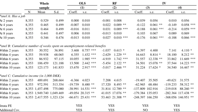
Our subsequent analysis of offenders’ post-sentencing labor market attachment confirms that custodial sentences increase the difficulties faced by offenders in the labor market as compared to non-custodial ones. Indeed, we find that incarceration significantly reduces offenders’ probability of having a job, increases their reliance on unemployment-related benefits, and, in fine, reduces their income. After 10 years, incarceration represents a cumulative loss of 368,056 kroners – corresponding to a 15.2% decrease at the mean, or one and a half year worth of income. The timing and nature of the effects suggest that difficulties in the labor market may explain part of the observed rise in criminal activities. More generally, these results also provide additional evidence that the social cost of incarceration can span beyond the mere period of incarceration, and suggest that the implementation of accompanying post-release measures may be necessary to mitigate these costs. Finally, we find substantial heterogeneity in our results based on offenders’ age and past labor market attachment as we show that our results are primarily driven by young offenders and, in particular, those who had a job at the end of the year preceding their crime. Presumably, these offenders were those who had the most to lose from being incarcerated at a time when they should have been strengthening their professional network and accumulating experience. The negative effects of custodial sentences (relative to non-custodial ones) are more limited on older offenders, as well as on those who were already struggling on the labor market.
Our findings contribute to the broad literature studying the social and economic effects of incarceration, both at the intensive margin (duration of prison time) and, more recently, at the extensive margin (incarceration versus alternative sanctions).6 Although longer incarceration spells may deter post-release criminal behavior (Drago et al., 2009), spending time in prison may also serve as a “school of crime” through exposure to other criminals, thus increasing future crime outcomes (Bayer et al., 2009; Stevenson, 2017; Piil Damm and Gorinas, 2020). Regarding labor market outcomes, incarceration has also been found to harm future employment prospects (see for instance Kling, 2006 or Mueller-Smith, 2015). Outside of the US, the literature is more limited and fails to reach a clear consensus. In a recent paper using Norwegian data, Bhuller et al. (2020) exploit the random allocation of criminal cases to judges with varying incarceration propensities and find that
5
former inmates recidivate less and face improved labor market outcomes when they were not employed prior to incarceration. However, alternative studies focusing on other Nordic countries and relying on a similar identification strategy reach contrasting conclusions that do not support the rehabilitative role of prison. In Sweden, Dobbie et al. (2018) find incarceration to have little impact on the probability for offenders to commit another crime, but a large negative impact on employment. In Denmark, Michel et al. (2019) find that incarceration increases the number of crimes offenders commit and reduces their labor market attachment. In these three Nordic studies, the results are identified on a very specific subsample of defendants at the margin of being incarcerated. By contrast, our paper focuses on a broader range of offender types arrested for a very widespread crime, i.e. drunk driving, thus enabling us to make a significant contribution to this debate in the context of a Nordic country. In this respect, our paper also relates to the literature looking at the effect of incarceration conditions, as we focus on a context where incarceration conditions are viewed as particularly exceptional by American and European standards (see for instance Pratt, 2008). Several studies, such as Chen and Shapiro (2007) for the US or Drago et al. (2011) for Italy, reveal that harsher prison conditions (measured by the intensity of security, the degree of social isolation, or inmates’ death rate for instance) increase post-release criminal activity. The recent study by Bhuller et al. (2020) in Norway rather suggests that when incarceration conditions are favorable, the rehabilitative effect of incarceration can dominate. Our results are instead surprisingly similar to those found in the US and imply that incarceration can remain a harmful experience with long term negative consequences even in Nordic countries.
Our study also makes an important side contribution as we show that individuals, especially wealthier ones, can anticipate the consequences of a reform and act upon it. Analyzing how the reform was implemented, we find evidence that offenders anticipated that they could avoid prison by postponing their trial until after the reform. In practice, these anticipations materialized through a sharp drop in the number of cases tried from the moment the law was signed (but before it actually entered into force), as well as a linear decrease in the share of defendants receiving a custodial sentence. We also show that wealthier defendants were more likely to “game the system” and avoid prison. To our knowledge, we are the first to provide such striking evidence in the context of a justice reform. These findings also suggest that traditional quasi-experimental estimators should be used with caution in similar contexts where salient contextual changes (such as a legislative reform, a program scale-up, etc.) can be anticipated by their stakeholders. Incidentally, our findings also question the degree of fairness with which cases can be handled in times of legislative changes and add to the growing
6
literature documenting sources of dysfunction in justice systems (Vidmar, 2011; Danziger et al., 2011; Abrams et al., 2012; Anwar et al., 2012; Anwar et al., 2014; Philippe and Ouss, 2018; Cohen and Yang, 2019).
The rest of the paper is organized as follows: in section 2, we provide contextual information and describe the reform under study; in section 3, we highlight the selection that occurred in the characteristics of offenders tried around the time of the reform; in section 4, we discuss our empirical strategy; in section 5, we present our results; finally, section 6 concludes.
2. The legislative change
2.1. Context of the reform
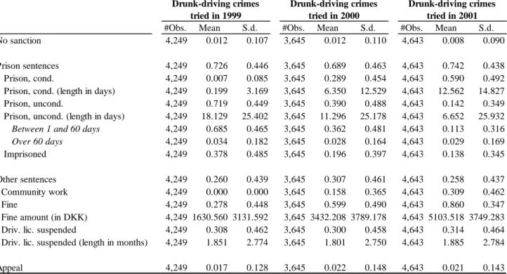
In the last quarter of the 20th century, legislations on drunk-driving crimes were gradually hardened throughout the world in an attempt to reduce the number of road fatalities. In Denmark, individuals arrested for drunk driving have been facing a prison sentence since the establishment of a first administrative blood alcohol threshold in 1976, lowered from 0.8 to 0.5g/L in 1998. In 1999, drunk driving was the crime responsible for the largest number of custodial sentences promulgated, accounting for 24.82% of them.
In 1999, the vast majority of individuals tried for a drunk-driving crime were convicted and incarcerated, as displayed in Table 1.7 In total, only 1.3% of the defendants tried were acquitted and 71.9% received an unconditional prison sentence. Although the severity of the sentence varied depending on the characteristics of the offense (e.g. driver’s level of impairment and existence of aggravating circumstances) and the number of prior drunk-driving convictions, the length of the incarceration spell remained relatively short: in 95.3% of the cases, it remained below 60 days. Additional sanctions, such as fines and suspensions of the driving license, were also frequently imposed on the defendant – in 27.8% and 30.8% of the trials respectively. Conversely, conditional prison sentences (probation) and community work were seldom used to sanction drunk drivers. For what follows, it is important to note that offenders suffering from an alcohol abuse problem who received a prison sentence of no more than 60 days could then ask to benefit from a pardon scheme described in Appendix A.1. As part of this scheme, their unconditional prison sentence could be commuted to a non-custodial sentence involving a two-year probation period and mandatory
7
participation in a yearlong rehabilitation program.This explains why the share of offenders who were actually incarcerated (37.8%) is lower than the share of those who received an unconditional prison sentence (71.9%).8
Offenders who served their prison sentence usually did so in one of the country’s open prisons.9 These prisons, which account for about a third of the total Danish prison capacity, are low-security facilities where fences, walls, and barriers are minimal, offering softer detention conditions for the inmates. Generally speaking, these detention facilities are meant to support the principle of normalization, officially introduced in Denmark in the early 1970s, according to which life in prison should reflect life outside and correspond as much as possible to conditions in the general community.
2.2. Details of the new law
In 2000, a reform was passed introducing cheaper, more lenient sentences against drunk drivers. As part of it, custodial sentences of no more than 60 days were replaced by a two-year probation period and a fine, combined with either community service or mandatory participation in a yearlong rehabilitation program (identical in every way to the one offered as part of the pardon scheme just mentioned above and described in Appendix A.1.).10,11 Following the reform, the average cost per offender decreased from 15.800 DKK (the cost of a custodial sentence) to 8.300 DKK (the cost of a non-custodial sentence) (Nielsen and Kyvsgaard, 2007).12
The choice between community service or mandatory participation in a rehabilitation program was left to the judges based on whether or not the offender suffered from an alcohol abuse problem, the rehabilitation program being reserved for offenders exhibiting such a problem. As part of this program, offenders had to take a drug causing acute sensitivity to Ethanol and to participate in an alcohol treatment program.13 Offenders were monitored throughout the duration of the treatment and the rest of the probation period.14 Probation officers were in charge of ensuring that the terms of the
8 Our variable indicating whether or not an individual was incarcerated is a dummy variable which captures whether an individual has
spent at least 10 days in prison – 10 days being the minimum duration of prison sentences requested for a drunk-driving crime.
9 Individuals serving a prison sentence inferior to four years and presenting no security threats to prison staff and other inmates are
usually incarcerated in open prisons. In practice, offenders incarcerated for 60 days or less cannot apply for early release on parole.
10 The only difference with the rehabilitation program implemented after the reform is that, until the 2000 reform, drunk drivers had to
apply to the Danish Prison and Probation Service to benefit from the pardon scheme. After the 2000 reform, it was left to the judge to decide whether or not an offender should enroll in the rehabilitation program.
11 Generally speaking, offenders placed on probation see their prison sentence suspended on the condition that they do not reoffend
and that they observe any conditions that may be imposed.
12 The cost of the non-custodial sentence includes the costs associated with offender supervision and the rehabilitation program. 13 In practice, this program could take a variety of forms (ranging from group sessions at a clinic to individual meetings with general
practitioners) and could vary in intensity depending on individuals’ location, needs, and motivation (Nielsen and Kyvsgaard, 2007).
14 During the first two months of the two-year program, offenders would usually meet with their probation officers every 2 weeks, but
8
probation were being respected and, in particular, of controlling offenders’ drug intake and participation in the alcohol treatment program during the first phase of the scheme. Community service was to be requested against offenders who did not exhibit such an alcohol abuse problem and was substituted to the former sentences at the following rate: 30 hours for 10 to 14 days of imprisonment, 40 hours for 20-30 day sentences, and 60 hours for 40 to 50 days in jail.15
As displayed in Table 1, the share of offenders who received an unconditional prison sentence dropped significantly after the reform, as intended: it fell from 71.9% in 1999 to 14.2% in 2001. Similarly, the share of offenders who were actually incarcerated decreased from 37.8% to 13.8%. In contrast, the share of offenders who received a conditional prison sentence and were placed on probation rose from 0.7% to 59.0%. As the reform did not change the punishments incurred by offenders facing no prison sentence, or by those facing more than 60 days of imprisonment (who kept on serving their prison sentence after the reform),16 the overall share of offenders who received a prison sentence (whether it be a conditional or an unconditional one) and the share of acquitted individuals remained similar before and after the reform. As expected, community work and fines were also imposed on a greater share of offenders after the reform. The use of driving license suspension was not impacted by the reform and is similar before and after it.
As detailed in the next section, the reform was perceived by offenders as a softening of the legislation, which is important to note for the interpretation of the results. Indeed, while the incarceration conditions in Scandinavian prisons are considered to be quite exceptional by American and European standards (Lappi-Seppälä, 2007; Pratt, 2008; Pratt and Eriksson, 2011; Ward et al., 2013), it is worth stressing that inmates remain subject to important freedom restrictions and other usual discomforts associated with imprisonment, even when they are incarcerated in an open prison. In particular, Basberg Neumann, a sociologist specializing in Nordic prisons and emphasizes the fact that inmates’ perception of prison conditions is largely determined by their frame of reference, namely the generous Scandinavian welfare system and institutions (Basberg Neumann, 2012). Importantly for the present study, social stigma upon release can play a major role in the rehabilitation process. In particular, suspended prison sentences remain on an individual's criminal record for 3 years from the conviction
15In case of mild violation(s) of the probation terms, the Prison and Probation Service decides whether or not to enforce the custodial
sentence. In case of more serious violation(s), judges are responsible for making the most appropriate decision.
16 Generally speaking, the reform applied to all offenders but extreme repeat drunk drivers and offenders facing extreme aggravating
circumstances. Also, it did not systematically apply to offenders who had already been placed on probation for a drunk-driving crime more than once or to those who were already on probation when they were apprehended for a drunk-driving crime.
9
date, while unconditional prison sentences stay on the record for 5 years from the date of release from prison.
3. Defendants anticipating the reform and gaming the system
As is often the case for important reforms that require a certain level of preparation, a few months elapsed between the moment the law was signed and the moment it entered into force. While the law was signed by Parliament on April 4th, 2000, it only entered into force on July 1st, 2000 (referred to as the date of the reform hereafter).
In this context, an important feature of Danish legislation lies in that it guarantees that defendants tried after a reform for a crime committed prior to it must be tried under the more lenient of the two laws – irrespective of the date of their crime. In practical terms, it means that individuals tried for a crime committed prior to the reform faced the risk of being incarcerated if tried before the reform, while they would be placed on probation if tried after. Thus, to the extent that defendants anticipated the reform and its consequences, they faced a clear incentive to try and postpone the date of their trial until after the reform in order to avoid prison. Below, we provide clear-cut evidence that this is precisely what happened with a large share of the drunk drivers postponing the date of their trial until after the reform. Crucially for our analysis, we further reveal that the characteristics of the individuals who gamed the system are not random and that wealthier defendants were more likely to do so.
3.1. Anticipation
First, we provide evidence that defendants anticipated the reform and modified their behavior from the moment the law was signed.
To do so, we use administrative data containing information on the universe of drunk-driving crimes committed and tried around the time of the reform to describe how the reform was implemented. In
Figure 1, we show the evolution of the following four indicators between 1999 and 2001: a) the
number of alleged drunk-driving crimes resulting in a trial committed every week; b) the number of drunk-driving cases tried every week in district courts; c) the share of defendants tried for driving who received a custodial sentence by week of trial; d) the share of defendants tried for drunk-driving who were actually incarcerated by week of trial. For each year, we draw two dotted vertical lines marking week 14 (the week when the law was signed in 2000) and week 26 (the week when it
10
entered into force in 2000). The only reform implemented during these three years occurred in 2000. For the years 1999 and 2001, vertical lines were only drawn for comparison purposes.17
Strikingly, the evolution of these indicators reveals that the way in which drunk-driving cases were handled in district courts changed drastically in the months following the signature of the reform and preceding its entering into force. Indeed, the number of cases tried each week dropped significantly from 91.7 cases on average in the three weeks preceding the signing of the law to 28.0 cases on average during the transition period (after the law was signed but before it entered into force) – representing a 69.5% decrease (Figure 1.b).18 This is the case despite the fact that there was no similar
variation in the number of alleged crimes resulting in a trial committed in the preceding months or in the number of cases tried during the same period in adjacent years, 1999 and 2001 (Figure 1.a).19
This suggests that stakeholders (courts of justice and/or defendants) anticipated the change in legislation and that, as a consequence, a large share of trials were postponed until after the reform. Hence, a group of offenders who should have been tried before the reform was tried after.20
The share of drunk drivers who received a custodial sentence (Figure 1.c) and the share of those who were actually incarcerated (Figure 1.d) also decreased substantially from the moment the bill was signed. This time, the decline did not take the form of a sharp discontinuity but rather of a linear decrease. Overall, the share of defendants receiving a custodial sentence decreased progressively from around 73.6% on average in the three weeks preceding the signing of the law to 34.5% on average in the three weeks preceding the date of the reform – representing a 53.1% decrease. Interestingly, while the evolution of the share of offenders actually incarcerated exhibits a similar pattern, it started to decrease a year before the date of the reform, suggesting that the Prison and Probation Service in charge of enforcing the sanctions may have anticipated the reform even further. Another possible explanation lies in the waiting list system adopted in Denmark after a sharp rise in
17 For data confidentiality reasons, indicators c) and d) displayed in Figure 1 are calculated as moving averages. For each year y, the
value of these indicators is calculated as the average value of the indicators over years y-1, y, and y+1.
18 The number of cases tried in the week following July 1st is low for all three years. This is a result of judges’ summer vacation period,
during which the number of cases tried in district courts goes down substantially.
19 In Appendix A.3., we also show that the reform did not have any impact either on the number of individuals charged for a
drunk-driving crime, which remained relatively constant prior to the reform, increased right after the signing of the reform, and progressively returned to its pre-reform level.
20 In total, assuming that the same number of drunk-driving cases were tried between weeks 14 and 26 in 1999, 2000, and 2001, we
estimate that roughly 48.1% of the drunk-driving cases which should have been tried during the transition period were in fact postponed until after the reform. In order to reach this figure, we assume that in the absence of the reform, the number of drunk-driving cases tried in 2000 would have been equal to the average number of such cases tried in the same weeks in 1999 (1,071) and 2001 (1,123) – 1,097. However, only 569 drunk-driving cases were tried during the transition period in 2000, suggesting that around 528 were postponed – which represents 48.1% of what would have been the total number of drunk-driving cases tried during that period.
11
the number of individuals who received an unconditional prison sentence. As a consequence, not all offenders served their prison sentence immediately after their trial.
Figure 1 – Implementation of the drunk-driving legislation reform: The consequences of the reform
are depicted here through the evolution of the following four indicators around the time of the change in legislation: a) the number of drunk-driving crimes resulting in a trial committed every week; b) the number of drunk-driving cases tried every week in district courts; c) the share of defendants tried for drunk-driving who received a custodial sentence by week of trial; d) the share of defendants tried for drunk-driving who were actually incarcerated by week of trial. For each year, the first dotted vertical line marks the week when the law was signed (week 14) and the second one marks the week when it entered into force (week 26).
While we are not able to pin down the exact underlying mechanisms at play here, we believe that both defendants and judges had incentives to postpone drunk-driving cases until after the reform. As already discussed above, defendants had an incentive to ask for the postponement of their trial to avoid prison. Interestingly, judges had an incentive to let them do so to reduce the number of cases
12
which might have to be retried. Indeed, Danish legislation also guarantees that defendants tried prior to the passing of a law lowering the sanction for the crime they were convicted of may request a retrial if they are still in prison (or on the waiting list to be incarcerated) when the reform enters into force.
3.2. Selection
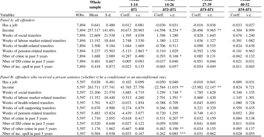
Going further, we investigate the characteristics of the defendants who acted in anticipation of the reform and got their case postponed, and find evidence suggesting that the selection was not random. To show this, we compare changes in the characteristics of the defendants tried in each quarter between 1999 and 2000. More specifically, focusing on individuals tried between January 1st, 1999 and December 31st, 2000, we regress different variables indicative of their criminal priors and labor market attachment on a constant, a year dummy indicating whether a case was tried in 2000, quarter fixed effects, the interactions between the year dummy and the quarter fixed effects, and a time trend. The coefficients associated with the year dummy thus capture differences in the characteristics of the defendants tried in the first quarter of 1999 and 2000, while the three interaction terms capture differential changes in the characteristics of the defendants tried in the first quarter and those tried in the 2nd, 3rd, and 4th quarters respectively. In particular, the coefficients associated with the interaction of the year and 2nd quarter dummies allow us to capture differential changes occurring during the
transition period (starting the week when the reform was signed and ending the week when it entered into force).
The corresponding estimates are reported in Table 2, along with the associated standard errors, clustered at the district court and individual levels. In Panel A, our sample includes all defendants tried during the period, while in Panel B, we focus on the subset of offenders who received a prison sentence (whether conditional or unconditional) as the group of defendants who had the most to gain from postponing the date of their trial.
While we do not find evidence of any change in the nature of the cases tried in the first and fourth quarters between 1999 and 2000 (columns 1 and 4), we find strong evidence of such a change occurring during the 2nd quarter of the year 2000 (column 2). Indeed, compared to those tried in the same quarter in 1999, we observe that defendants tried during the transition period, especially those who received a prison sentence, had weaker ties to the labor market: they had lower income and were more likely to receive benefits, particularly unemployment-related benefits. While the effects are diluted when we focus on the entire sample of defendants tried during the period, the magnitude of
13
the differences is particularly important and significant for the restricted subset of defendants who received a prison sentence and had something to gain from postponing their trial. For instance, at the sample mean, the income of the defendants who received a prison sentence dropped by 8.6 percentage points during the transition period. Overall, this suggests that wealthier individuals were more often able to postpone their case until after the reform than other defendants – presumably because they had access to better legal counsel.
We can rule out the possibility that this selection merely reflects an attempt to focus on offenders whose trial outcome did not depend on the timing of the trial during the transition period. For instance, we do not observe any change in the average number of drunk-driving crimes committed by offenders tried during the transition period, although the reform did not apply systematically to repeat drunk-drivers.21 Overall, we actually find that defendants tried during the transition period tended to be more severe offenders. On average, individuals tried in the 2nd quarter of the year 2000 had been convicted and incarcerated a greater number of times for crimes other than drunk driving. Again, the magnitude of the differences is particularly important and significant for the subset of offenders who received a prison sentence. For instance, at the sample mean, they represent increases of 31.0% in the number of crimes and of 52.0% in the number of incarceration spells recorded by the defendants in the previous 5 years. These results further suggest that defendants tried during the transition period were in a more precarious situation.
Finally, we still observe some compositional changes for the third quarter (column 3) but they merely reflect the fact that the number of cases remained lower than usual in the aftermath of the reform – as displayed in Figure 1.b.
Overall, these findings question the degree of consistency with which drunk-driving cases were handled in district courts, as well as the level of fairness with which defendants were treated by the justice system during the transition period. From a methodological point of view, our results suggest that the way drunk-driving cases were handled in district courts during the transition period generated differences in the nature of the defendants tried before and after the reform. This also raises questions
21 Offenders who had already been placed on probation for a drunk-driving crime more than once or who were on probation at the time
14
with respect to the performance of traditional quasi-experimental estimators in the context of this reform and other similar ones.22
4. Empirical strategy
In order to measure the causal impact of the reform and bypass the selection problem documented above, we use a novel instrumental variable relying on variation in the probability for offenders to receive a custodial sentence. This variation, which we argue is plausibly exogenous, is generated by the time lapse between the date of their crime and the date when the reform entered into force.
4.1. The intuition behind the instrument
Our approach relies on two features of the justice system which, when combined together, create exogenous variation in the probability for offenders to receive a custodial sentence. The first of these features is the fact that, as already mentioned above, Danish legislation guarantees that defendants tried after a reform for a crime committed prior to it must be tried under the more lenient of the two laws. It means that individuals tried after July 1st, 2000 for a drunk-driving crime committed before that date were tried under the new law. The second of these two features is the significant time gap between the moment a crime is committed and the moment the corresponding decision of justice is rendered by a district court – as further documented below. Together, these features ensure that the closer to the reform a crime was committed, the more likely the offender was to be tried after the reform under the new law, and therefore to avoid prison.
In Figure 2, we provide evidence of the strength of this approach. In order to do so, we organize the data based on the week when the crime was committed (hereafter referred to as “week of crime”), instead of the week when the sentence was rendered, and depict the following indicators: a) the average time gap between the moment an alleged crime was committed and the moment the decision of justice was rendered by a district court by week of crime; b) the share of cases tried after July 1st,
22 Traditional quasi-experimental estimators raise additional selection problems which, although not discussed in details here, remain
essential. In particular, one concern is that the entering into force of the new law might have been accompanied (at least for a time) by more frequent police controls to compensate for the reduction in the expected costs of the punishment by increasing the probability of being caught drunk driving. Moreover, another concern is that potential offenders might have modified their behavior around the time of the reform. For instance, they might have anticipated the above-mentioned increase in road traffic controls and behaved more carefully in the weeks following the entering into force of the reform, thus reducing the overall number of drunk-driving crimes. Furthermore, conditional on individuals internalizing changes in the legislation, the reform should also have induced a modification in the characteristics of the individuals arrested for a drunk-driving crime after the law was passed. Indeed, the lowering of the cost associated with drunk-driving crimes should mechanically have led a new range of individuals to commit drunk-driving crimes (those reaping lower benefits from committing a crime and/or incurring higher costs if caught), thereby increasing the overall number of drunk-driving crimes.
15
2000 (the date when the reform officially entered into force) by week of crime; c) the share of defendants tried for an alleged drunk-driving crime who received a custodial sentence by week of
crime; d) the share of defendants tried for an alleged drunk-driving crime who were actually
incarcerated by week of crime.23
The evolution of the first two indicators provides graphical support for our approach. Around the time of the reform, the period of time between the moment when a prosecutor would press charges against an alleged drink-driver and the moment when a district court rendered its decision was substantial. On average, the time gap was of 6 months for drunk-driving crimes committed in 1999 and it increased for crimes committed closer to the reform (Figure 2.a). This time gap was almost entirely driven by the case processing time in district courts. As a consequence, as individuals’ arrest date got closer to the reform within the 12-month period preceding it, an increasingly large share of them was tried after, under the new law (Figure 2.b).
As for the last two indicators, their evolution confirms that there was significant variation in the probability of receiving a custodial sentence among individuals tried for a drunk-driving crime committed in the 12-month period preceding the reform, based on the date of their crime. Indeed, the share of defendants who received a custodial sentence by week of crime started going down from July 1999 from slightly less than 80% to less than 20% right after the reform (Figure 2.c). The same pattern is observed for the share of defendants who were actually incarcerated following their trial – although the decrease starts earlier (Figure 2.d).
23 For data confidentiality reasons, indicators c) and d) displayed in Figure 2 are calculated as moving averages. For each year y, the
value of these indicators is calculated as the average value of the indicators over years y-1, y, and y+1. Furthermore, for any given week, the number of cases tried after the reform is normalized to 1 if the actual number of cases tried after is equal to or lower than 3 (in total, this normalization was carried out for 16 weeks), and the number of cases tried after the reform is normalized to 1 if the actual number of cases tried before is equal to or lower than 3 (in total, this normalization was carried out for 4 weeks).
16
Figure 2 – Motivation for the instrumental variable approach: This figure depicts
the evolution of the following four indicators around the time of the reform: a) the average time gap between the moment a crime is committed and the moment the decision of justice is rendered by a district court by week of crime; b) the share of cases tried after July 1st, 2000 (the date when the reform officially entered into force) by week
of crime; c) the share of defendants who received a custodial sentence by week of crime;
d) the share of defendants who were actually incarcerated by week of crime. For each year, the first dotted vertical line marks the week when the law was signed (week 14) and the second one marks the week when it entered into force (week 26).
17 4.2. Sampling strategy
Our approach therefore compares individuals who committed their drunk-driving crime before the signature of the reform based on the date of their crime.
In what follows, we focus on all individuals charged for a drunk-driving crime committed in the
24-month period preceding the signing of the law (between week 15 of 1998 and week 14 of 2000).24
While Figure 2 shows that our instrument exhibits no variation among individuals charged for a drunk-driving crime committed 13 to 24 months before the entering into force of the reform (between week 15 of 1998 and week 14 of 1999), these individuals are included in our sample as well so as to control for seasonal variations using both a time trend, year and month fixed effects. Restricting our sample to defendants tried in the country at that time, we obtain a sample of 8,353 cases, corresponding to 7,959 distinct defendants.25
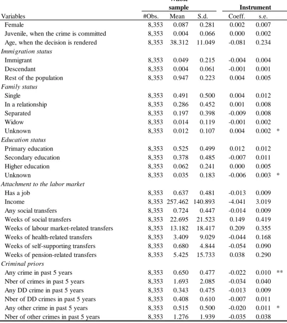
In Table 3, we provide a description of the characteristics of the defendants included in our sample. They are predominantly males in their late thirties. While close to 63.7% of them held some type of job at the end of the year preceding the date of their crime, 72.4% received social benefits in the 12-month period preceding their crime. On average, defendants received transfers for 22.7 weeks, with unemployment-related benefits alone accounting for 13.2 weeks. Strikingly, 34.3% of the defendants had already had at least one conviction for a drunk-driving crime in the previous 5 years. Few of them are in a relationship (28.6%), and defendants born abroad and descendants of immigrants represent 4.9% and 0.4% of the sample respectively – slightly less than their actual share in the overall population in 2000, which was 5.4% and 1.4% respectively.
4.3. Econometric specifications RF and IV approaches
In order to report on the impact of the reform, we show the reduced form estimates (RF) derived from the estimation of the following equation:
𝑦𝑖,𝑡 = 𝛿𝑅𝐹(𝑃⏞ 𝑖 ∗ 𝑇𝑖
𝐼𝑖
) + 𝑋𝑖𝛽 + 𝜇1𝑇𝑖 + 𝜇2𝑃𝑖 + 𝜇𝑚+ 𝜇𝑐+ 𝜀𝑖 (1)
24 More information on the administrative datasets used as part of this study can be found in Appendix A.2.
25 In the few cases where an individual had allegedly committed more than one drunk-driving crime throughout the study period,
keeping only the case associated with the first alleged drunk-driving crime yields results similar to those displayed below (results are available upon request).
18
where 𝑦𝑖,𝑡 is the outcome of interest for individual i measured at time t; 𝑇𝑖 is a trend, increasing with time, which captures the time gap between the moment when the crime was committed and the date of the reform (the unit for this variable is 100 days);26 𝑃𝑖 is a period dummy taking the value 1 if individual i’s crime was committed in the 12-month period preceding the reform and 0 if it was committed earlier; 𝜇𝑚 and 𝜇𝑐 are fixed effects indicating the month when individual i committed their crime and the district court where they were tried (there are 84 of them); and 𝑋𝑖 is a vector including
all variables in the conditioning set detailed in Appendix A.2.27 Because drunk-driving behavior may vary endogenously with the day of the week when the crime is committed (e.g. weekdays versus weekends), we also tried an alternative specification where we include day of the week fixed-effects.28
Our instrument, 𝐼𝑖 = (𝑃𝑖 ∗ 𝑇𝑖), captures the differential effect of the 𝑇𝑖 variable for crimes committed
in the 12-month period preceding the day the reform entered into force, when compared to crimes committed in the 13 to 24 months before the reform. The parameter of interest is 𝛿𝑅𝐹, which should be different from 0 if the nature of the sanctions imposed on offenders before and after the reform has an impact on 𝑦𝑖,𝑡, as the probability of receiving a custodial sentence is positively correlated with the time gap between the moment the crime was committed and the entering into force of the reform in the 12-month period preceding it. In contrast, Figure 2 suggests that there is no particular reason to expect 𝜇1 to be statistically different from 0.
The estimates we focus on most closely are our IV estimates, which we obtain by instrumenting 𝑐𝑢𝑠𝑡𝑖, a dummy variable indicating whether individual i received a custodial sentence as part of their trial, by our instrument 𝐼𝑖 using a Two-Stage-Least-Squares estimation procedure. Coefficients 𝛿𝐼𝑉
measure the impact of receiving a custodial sentence (as opposed to a non-custodial one) on the
compliers, the subset of defendants whose time of crime within the 12-month period preceding the
26 𝑇
𝑖is a time trend, rather than the time gap between the moment when the crime was committed and the date of the reform, to avoid
violating the monotonicity assumption – which will be discussed below. Hence, 𝑇𝑖 is constructed in such a way that the greater its value is, the closer to the reform individual i committed their crime.
27 We control for various trial characteristics, such as whether the defendant was a juvenile at the time of the crime and the nature of
the main charge (using a detailed 7-digit drunk-driving charge code). We also include defendants’ background information, such as their gender, age at the time of the trial, immigration status (as per Statistics Denmark’s typology: “immigrants”, “descendant of immigrants”, or “rest of the population”), their past criminal activity (the number of convictions for other drunk-driving crimes, other road traffic crimes, and non-road traffic crimes in the 5-year period preceding their crime), marital status, highest educational achievement, type of job held, and annual earnings (before tax and any social contributions). Unless specified otherwise, all baseline background characteristics included in the conditioning set were measured at the end of the year preceding the crime and are available for the vast majority of the offenders in our sample (the variables included in the conditioning set are all available from 1986).
19
entering into force of the reform had an impact on whether or not they received a custodial sentence – i.e. offenders who were sentenced to serve 1 to 60 days in prison.
Standard OLS approach
For comparison purposes, we also show the standard Ordinary-Least-Squares estimates (OLS) we obtain when estimating the following linear model:
𝑦𝑖,𝑡 = 𝛿𝑂𝐿𝑆𝑐𝑢𝑠𝑡
𝑖 + 𝑋𝑖𝛽 + 𝜇1𝑇𝑖+ 𝜇2𝑃𝑖 + 𝜇𝑚+ 𝜇𝑐 + 𝜀𝑖 (2)
In this equation, the coefficient 𝛿𝑂𝐿𝑆 is the parameter of interest. However, for a number of reasons, the 𝑐𝑢𝑠𝑡𝑖 variable is likely to be endogenous in this specification. Indeed, as displayed in Table 3, offenders who receive a custodial sentence and those who receive a non-custodial one differ significantly and, unless all differences across these two groups are controlled for (which seems unlikely to occur), these OLS estimators are likely to yield biased estimates.
4.4. Instrument validity
First-stage and compliers’ characteristics
In Table 4, we estimate the impact of having committed a drunk-driving crime closer to the signing of the law on the probability for a defendant to receive a custodial sentence (Panel A) and on the probability for a defendant to actually be incarcerated, as measured by our proxy (Panel B). In order to do so, we regress the binary variable indicative of the trial outcome on our instrument and an increasingly exhaustive set of control variables. From column 1 to column 4, we enrich the set of control variables by adding the following covariates successively and incrementally: a time trend, period, month-of-crime and district court fixed effects (column 1), dummy variables indicative of the nature of the drunk-driving charge (column 2), information about the criminal case (column 3), and defendant characteristics (column 4).
As expected, we find that having committed a crime closer to the moment when the law was signed substantially reduces the probability of receiving a custodial sentence for a crimecommitted in the 12-month period preceding the entering into force of the reform (Panel A). Indeed, within that period, delaying their drunk-driving crime by 100 days would have reduced defendants’ probability of receiving a custodial sentence by 14.5 percentage points. Furthermore, both the magnitude and significance level of these estimates are robust to the inclusion of covariates in the regression, suggesting that, in the 12-month period preceding the signing of the law, the time gap between the
20
day a defendant supposedly committed their crime and the moment when the law was signed is independent of their characteristics and those of their case.
Similarly, we find that delaying their drunk-driving crime by 100 days would have reduced defendants’ probability of being incarcerated by 7.0 percentage points in the 12-month period preceding the entering into force of the reform (Panel B). As already discussed above, the difference in the magnitude of the first-stage estimates displayed in Panels A and B can be explained by the implementation of the pardon scheme prior to the reform and by the prison waiting list.
In Appendix A.4, we describe the characteristics of the offenders whose date of crime had an impact on whether or not they received a prison sentence. To do so, we use the methodology followed by Pinotti (2017), which consists in eliciting compliers’ characteristics by the 2SLS regression of the product of the individual characteristics and the endogenous variable on the endogenous variable using I as an instrument. We find that the characteristics of the first group are very similar to those of the overall sample. This suggests that the selection described in section 3 does not affect the characteristics of the compliers.
Independence, exclusion, and monotonicity
However, for this instrument to be valid, it also has to meet the following standard conditions: independence, exclusion, and monotonicity.
The independence assumption implies that the instrument is independent of defendants’ background characteristics and potential outcomes (once a time trend, period, month-of-crime and district court fixed effects are controlled for). In order to further investigate the validity of this assumption, we study whether or not defendants’ pre-crime characteristics are correlated with the instrument. We do so by regressing each of the background variables displayed in the left column of Table 3 on the instrument, the time trend, as well as period, month-of-crime and district court fixed effects. For each regression, we report the coefficient and standard error associated with the instrument in Table 3. We find that the coefficients associated with the instrument are systematically small and largely insignificant, indicating that the independence assumption is likely to be met.29 This also suggests that the reform was not anticipated by potential offenders prior to the date of its signature.
29 In what follows, we also show that the IV estimates are very similar irrespective of whether or not the conditioning set is included
21
The exclusion restriction implies that the timing of the crime itself does not have any direct impact on our outcome variables (defendants’ crime and labor outcomes up to ten years after the completion of their trial). One concern is that the risk of recidivism and/or prospects of employment might vary across defendants based on the timing of their crime or the date of their sanction. However, the inclusion in our sample of individuals tried for a drunk-driving crime committed 13 to 24 months before the reform allows us to mitigate the consequences of this potential problem by controlling for trend and seasonality effects.
Finally, the monotonicity assumption implies that the probability of receiving a custodial sentence decreased for all offenders as their crime was committed closer to the reform in the 12 months preceding it. While nothing in the implementation of the reform leads us to suspect otherwise, we investigate the validity of this assumption by estimating the first-stage equation for various subgroups of the sample: males, females, individuals aged below 30, individuals aged above 30, individuals with prior drunk-driving convictions, individuals without any prior drunk-driving convictions, etc. The coefficients and standard errors associated with each of the subgroups are reported in Appendix A.5. We find that the coefficients are all positive and statistically significant (as well as very similar in magnitude). This suggests that problems arising due to non-monotonicity are probably limited as well.
5. Main Results
We measure the relative impact of custodial and non-custodial sentences on offenders’ post-sentencing outcomes using the strategy described in the previous section. We investigate their impact on offenders’ subsequent criminal behaviors and labor market attachment.
5.1. Impact on crime Overall impact
We start by measuring the relative impact of custodial and non-custodial sentences on drunk drivers’ post-sentencing involvement in criminal activities.30 In Figure 3, we report on the differential effect
of the two sentences as measured by our IV estimates. To do so, we compute the following two cumulative outcomes every 3 months from the date when the drunk-driving case was settled in court:
30 In order to measure the net impact of incarceration, we exclude from the calculation of these outcomes any crime registered under
22
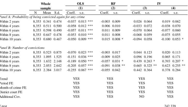
a) the probability of being convicted of a crime by time t (the extensive margin); and b) the number of convictions committed by time t (the intensive margin). All subsequent convictions (for all types of crimes) are included in the calculation of these outcomes. A subset of coefficients is displayed in
Table 5.
Although standard errors are large, several overall patterns emerge. At the extensive margin, our results suggest that custodial and non-custodial sentences are equally effective in preventing offenders from being reconvicted (Figure 3.a). Throughout most of the study period, point estimates are close to 0 and fail to be statistically significant at the 10% level. It is only towards the end of the period that estimates start to suggest that incarceration may become a little more effective in reducing the share of offenders who are reconvicted in the long run, as point estimates become statistically significant at the 10% level.
Turning to the intensive margin, we find that custodial sentences significantly increase the average number of convictions (Figure 3.b). At its peak, the magnitude of the effect is quite large: our results indicate that incarceration increases the average number of convictions by 0.623 crime after 8 years – representing a 30.3% increase at the sample mean. Because we do not find any effect on the extensive margin, the effect at the intensive margin is mechanically larger on reoffenders – individuals who were reconvicted at least once. Hence, it seems that while incarceration does not increase the number of reoffenders, it intensifies their subsequent criminal activities. It is also important to note that offenders’ number of convictions following their trial is top-coded at the 99th percentile (see Appendix A.2.). Therefore, we are confident that having significant estimates at the intensive margin, but no significant effect at the extensive margin is not simply driven by extreme values.
Taking a closer look at the results, a first interesting pattern lies in the sudden drop experienced by point estimates one to two years after the trial, which suggests that incarceration is more effective in preventing criminal behaviors than probation in the very short run. The bottom is reached after 15 months, at which point the extensive margin coefficient is statistically significant at the 5% level and the intensive margin coefficient at the 10% level. We interpret this pattern as reflecting the incapacitation effect of custodial sentences and its late timing as the consequence of the waiting list system in effect at the time, which could delay offenders’ incarceration up to several months after the promulgation of their sentence.
23
Figure 3 – Impact of custodial vs. non-custodial sentences on crimes: This figure
depicts the cumulative impact of a custodial sentence (as measured by our IV estimates) on the following outcomes: a) the probability of being convicted of a crime; and b) the number of convictions. Crime outcomes are measured every 3 months from the date when the drunk-driving case was settled in court.
The timing of the effects during the rest of the study period is also quite revealing at the intensive margin. First, the impact of the two sanctions is remarkably similar during the following two years, with differences remaining small in magnitude and non-statistically significant. It is only from the 5th year after the decision of justice that the negative effect of incarceration really begins to materialize. This may be so for a number of reasons, including the length of the non-custodial sentence and requirements associated with it. It is also interesting to note that conditional sentences remain on offenders’ criminal record for 3 years from the date of their trial. We interpret this as a sign that
non-24
custodial sentences represent an important disruption in individuals’ lives. In particular, the stigma associated with having a criminal record (as revealed by Pager, 2003; Raphael, 2014; Agan and Starr, 2018 and Mueller-Smith and Schnepel, 2020) would disappear three years after trial for individuals placed on probation, but would last up to five years after release for those incarcerated, consistent with the patterns observed in the data. Finally, the difference in the effects of the two sanctions reaches its maximum 8 years after the decision of justice and starts diminishing from then on, implying that, relatively speaking, the negative effects of custodial sentences can dissipate.However, for most offenders this coincides with the start of the 2008 economic crisis and the rise in unemployment. This pattern will be commented further below, but these results suggest that the impact of custodial and non-custodial sentences may depend on the peculiarities of the legal sanctions, as well as on external factors.
In comparison with IV and reduced-form estimates, the standard OLS approach yields very different results. As displayed in Table 5, we find that OLS estimates suggest that there is a negative relationship between receiving a custodial sentence and crime, both at the extensive and intensive margins. Consistent with the deterrence theory, these coefficients suggest that custodial sentences decrease both the probability for a drink-driver to be subsequently convicted of any other crime, as well as the number of such crimes they commit. For instance, they suggest that custodial sentences decrease the probability for an offender to commit any other crime within the next 10 years by 5.0 percentage points (representing a 7.4% decrease at the sample mean) and reduces the number of such crimes they commit by 0.255 crime (representing a 10.7% decrease at the sample mean). Both results are statistically significant at the 1% level. The differences between standard OLS and IV results cast further doubt on the reliability of studies attempting to mitigate the differences across groups by controlling for observable confounding factors.
Overall, our results provide evidence that non-custodial sentences can be at least as effective as custodial ones to prevent subsequent crime. From policymakers’ perspective, our results also provide supporting evidence that non-custodial sentences can be more cost-effective than custodial ones to reduce subsequent crime.
Rehabilitative or criminogenic effect?
The above results suggest that in the long run, probation leads to fewer crimes compared to incarceration. A natural question is whether this effect is driven by the positive impact of the
25
rehabilitation program offered to some offenders placed on probation to deal with their alcohol abuse problem, or rather by a criminogenic effect of incarceration.
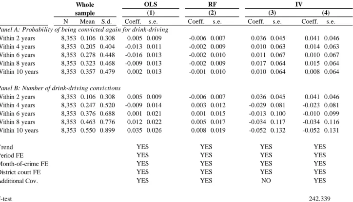
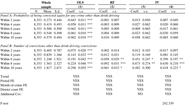
To answer this question, we split our overall crime outcomes between convictions for a drunk-driving crime and convictions for any other crime, and report on the relative impact of custodial and non-custodial sentences on these two types of convictions in Figure 4. We use the first outcome to test whether or not non-custodial sentences had any differential rehabilitative effect on offenders’ alcohol abuse problem. We use the second outcome to test whether or not incarceration had a criminogenic effect. Again, we measure their relative impact on the extensive and intensive margins every 3 months from the date when the drunk-driving case was settled in court. A subset of coefficients is displayed in Tables 6.
We find no differential impact on convictions for drunk-driving crimes, suggesting that the increase in the number of convictions cannot be driven by the positive effect the rehabilitation program may have had on the alcohol abuse problem of offenders placed on probation. Indeed, the two sanctions appear to be equally effective in preventing offenders from being reconvicted for a drunk-driving crime (Figure 4.a), and their impact on the average number of convictions for drunk driving is also similar (Figure 4.c). In both cases, point estimates are relatively small in magnitude and systematically fail to be statistically significant at the 5% level. This is so despite significant room for improvement. As displayed in Tables 6, the average number of reconvictions for a drunk-driving crime for individuals included in our sample is 0.6 after 10 years. To some extent, the absence of a rehabilitative effect may be explained by the fact that, as mentioned above, the rehabilitation program was only offered to a subset of offenders placed on probation (those who suffered from an alcohol abuse problem). Moreover, these offenders could already benefit from it prior to the reform (they only had to request it). As a consequence, the number of compliers who benefitted from the rehabilitation program may be too limited for its positive effect (if any) to materialize in our results. In contrast, our results highlight the criminogenic effect of incarceration as we find that, compared to non-custodial sentences, custodial ones increase the average number of convictions for crimes other than drunk driving (Figure 4.d). At its peak, the magnitude of the effect is large: our results indicate that custodial sentences increase the average number of convictions by 0.630 crime after 8 years – representing a 40.3% increase at the sample mean. Because custodial and non-custodial sentences appear to be equally effective in preventing individuals from being convicted for a crime other than
26
drunk driving (Figure 4.b), the effect on the intensive margin is again mechanically larger on offenders who were convicted at least once.
Figure 4 – Impact of custodial vs. non-custodial sentences on drunk-driving and other crimes:
This figure depicts the cumulative impact of custodial sentences (as measured by our IV estimates) on the following outcomes: a) the probability of being convicted of a drunk-driving crime ; b) the probability of being convicted of any other crime; c) the number of convictions for a drunk-driving crime; and d) the number of convictions for any other crime. Crime outcomes are measured every 3 months from the date when the drunk-driving case was settled in court.
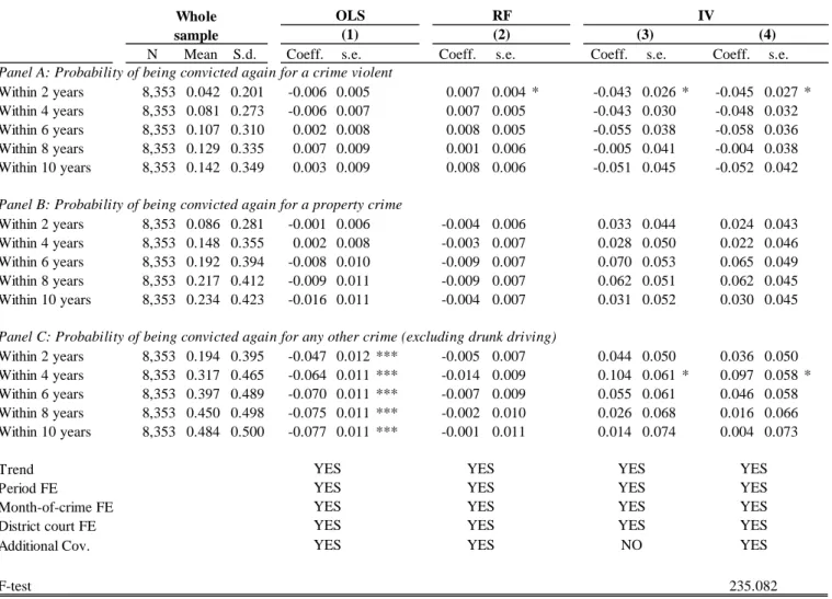
When further disaggregating the type of other crimes committed, we find that our results are driven by economically motivated crimes. In Figure 5, we report on the relative impact of custodial and non-custodial sentences on convictions for violent, property, and other crimes taken separately, leaving drunk-driving crimes out of this analysis. A subset of coefficients is displayed in Tables 7. We observe a strong and particularly significant increase in the number of convictions for property crimes. In contrast, we do not find any impact on the number of convictions for violent crimes. While incarceration seems to increase the number of convictions for other crimes, point estimates fail to be statistically significant at the 5% level, making it harder to draw more definitive conclusions. Overall, these results suggest that incarceration may significantly weaken the labor market attachment of offenders who, to a larger extent, resort to crime to make a living – a theory we investigate further in the next section.