Comparison of co-located independent ground-based middle atmospheric wind and temperature measurements with numerical weather prediction models

(1)

HAL Id: insu-01180350

https://hal-insu.archives-ouvertes.fr/insu-01180350

Submitted on 20 Aug 2020

HAL is a multi-disciplinary open access

archive for the deposit and dissemination of

sci-entific research documents, whether they are

pub-lished or not. The documents may come from

teaching and research institutions in France or

abroad, or from public or private research centers.

L’archive ouverte pluridisciplinaire HAL, est

destinée au dépôt et à la diffusion de documents

scientifiques de niveau recherche, publiés ou non,

émanant des établissements d’enseignement et de

recherche français ou étrangers, des laboratoires

publics ou privés.

middle atmospheric wind and temperature

measurements with numerical weather prediction models

Alexis Le Pichon, J. D. Assink, P. Heinrich, E. Blanc, Andrew J.

Charlton-Perez, C.-F. Lee, Philippe Keckhut, Alain Hauchecorne, Rolf

Rüfenacht, Niklaus Kämpfer, et al.

To cite this version:

Alexis Le Pichon, J. D. Assink, P. Heinrich, E. Blanc, Andrew J. Charlton-Perez, et al.. Comparison

of co-located independent ground-based middle atmospheric wind and temperature measurements

with numerical weather prediction models. Journal of Geophysical Research: Atmospheres, American

Geophysical Union, 2015, 120 (16), pp.8318-8331. �10.1002/2015JD023273�. �insu-01180350�

(2)

Comparison of co-located independent ground-based middle

atmospheric wind and temperature measurements

with numerical weather prediction models

A. Le Pichon1, J. D. Assink1, P. Heinrich1, E. Blanc1, A. Charlton-Perez2, C. F. Lee2, P. Keckhut3, A. Hauchecorne3, R. Rüfenacht4, N. Kämpfer4, D. P. Drob5, P. S. M. Smets6,7, L. G. Evers6,7, L. Ceranna8, C. Pilger8, O. Ross8, and C. Claud9

1

CEA, DAM, DIF, Arpajon, France,2Department of Meteorology, University of Reading, Reading, UK,3LATMOS-IPSL, Guyancourt, France,4_{Institute of Applied Physics, Bern University, Bern, Switzerland,}5_{Geospace Science and Technology}

Branch, Space Science Division, Naval Research Laboratory, Washington, DC, USA,6Seismology and Acoustics, KNMI, De Bilt, Netherlands,7_{Department of Geoscience and Engineering, Delft University of Technology, Delft, Netherlands,}8_{BGR, B4.3,}

Hannover, Germany,9LMD/IPSL, Ecole Polytechnique, Palaiseau, France

Abstract

High-resolution, ground-based and independent observations including co-located wind radiometer, lidar stations, and infrasound instruments are used to evaluate the accuracy of general circulation models and data-constrained assimilation systems in the middle atmosphere at northern hemisphere midlatitudes. Systematic comparisons between observations, the European Centre for Medium-Range Weather Forecasts (ECMWF) operational analyses including the recent Integrated Forecast System cycles 38r1 and 38r2, the NASA’s Modern-Era Retrospective Analysis for Research and Applications (MERRA) reanalyses, and the free-running climate Max Planck Institute–Earth System Model–Low Resolution (MPI-ESM-LR) are carried out in both temporal and spectral domains. Weﬁnd that ECMWF and MERRA are broadly consistent with lidar and wind radiometer measurements up to ~40 km. For both temperature and horizontal wind components, deviations increase with altitude as the assimilated observations become sparser. Between 40 and 60 km altitude, the standard deviation of the mean difference exceeds 5 K for the temperature and 20 m/s for the zonal wind. The largest deviations are observed in winter when the variability from large-scale planetary waves dominates. Between lidar data and MPI-ESM-LR, there is an overall agreement in spectral amplitude down to 15–20 days. At shorter time scales, the variability is lacking in the model by ~10 dB. Infrasound observations indicate a general good agreement with ECWMF wind and temperature products. As such, this study demonstrates the potential of the infrastructure of the Atmospheric Dynamics Research Infrastructure in Europe project that integrates various measurements and provides a quantitative understanding of stratosphere-troposphere dynamical coupling for numerical weather prediction applications.

1. Introduction

Weather and climate forecasting communities are moving toward a more comprehensive representation of the atmosphere to better capture stratospheric-tropospheric interactions and improve long-term forecasts. The combination of innovative relevant observations and numerical modeling contribute to a better predic-tion of extreme atmospheric events. An important part of improving our understanding of the general circulation of the middle atmosphere (MA, from ~12 to 90 km) is building a detailed knowledge of the MA dynamics through multiple complementary observational platforms.

In recent years, general circulation models (GCMs) have been progressively extended higher to cover the whole stratosphere and in some cases the mesosphere, because it is now recognized that stratospheric circulation anomalies, often formed in the mesosphere and the lower thermosphere (MLT) [Coy et al., 2011; Angot et al., 2012], may affect tropospheric weather on time scales from weeks to months [e.g., Baldwin et al., 2003; Charlton-Perez et al., 2004]. The MLT is a dynamic medium with variability over time scales ranging from minutes to days. Both the mean state and the variability within the MLT are subject to inaccuracies both in current operational analyses and reanalyses [Rienecker et al., 2011; Hoppel et al., 2013].

The majority of assimilated observations are satellite-based radiances that often include a signiﬁcant contri-bution from the upper stratosphere and lower mesosphere. They have their most direct effect in the

Journal of Geophysical Research: Atmospheres

RESEARCH ARTICLE

10.1002/2015JD023273 Key Points:

• ECMWF and MERRA agree with wind and temperature observations up to 40 km

• Above 30 km, a climate and two NWP models underestimate 2–15 day variability

• Independent instruments are used to validate GCMs in the middle atmosphere

Supporting Information:

• Table S1 and Figures S1–S4

Correspondence to:

A. Le Pichon, alexis.le-pichon@cea.fr

Citation:

Le Pichon, A., et al. (2015), Comparison of co-located independent ground-based middle atmospheric wind and temperature measurements with numerical weather prediction models, J. Geophys. Res. Atmos., 120, 8318–8331, doi:10.1002/2015JD023273.

Received 18 FEB 2015 Accepted 20 JUL 2015

Accepted article online 23 JUL 2015 Published online 28 AUG 2015

(3)

troposphere and lower stratosphere (i.e., below ~35 km) because their weighting function peaks are gener-ally in those regions [Hoppel et al., 2013]. There are no direct routinely operational meteorological wind measurements presently available above ~30 km where few radiosondes reach; thus, winds are derived from thermal wind balance and wind data assimilated at lower levels. Generally, winds are adjusted as part of the assimilation system, so that winds and temperatures are approximately in balance before a model forecast begins [Polavarapu et al., 2005].

Assimilation of temperatures in the MA into current operational models is still developing for a number of reasons [Hoppel et al., 2013]: (i) satellite observations with weighting functions that peak in the mesosphere are typically not provided in real time as most of these observations come from research instruments, (ii) biases in the assimilation of satellite radiance observations [Derber and Wu, 1998], and (iii) data assimilation systems are affected by the different biases originating from the combination of multiple data sources or by limitations of the assimilating model [Dee, 2005; Polavarapu et al., 2005].The assimilation of these data in reanalyses up to an ~50 km altitude further inﬂuences upper regions through model calculations [Sakazaki et al., 2012].

In earlier studies, comparison of these satellite observations with model output in the MLT region has been performed over monthly time scales [Rienecker et al., 2011; Sakazaki et al., 2012] to reconcile the temporal and spatial sampling differences of the two techniques [Wendt et al., 2013]. Rienecker et al. [2011] and Kishore Kumar et al. [2014] have shown that biases may exceed a few tens of meters per second for winds and 10 K for temperatures in the monthly means. Comparisons of windﬁelds in the MA from global meteorological data assimilation systems to satellite observations are somewhat limited. Recent studies include comparisons between output from the European Centre for Medium-Range Weather Forecast (ECMWF) analysis with obser-vations from long-duration balloons [Podglajen et al., 2014] and from the Superconducting Submillimeter-Wave Limb-Emission Sounder research instrument on board the international space station [Baron et al., 2013]. Earlier validations also include rocketsonde measurements [e.g., Hamilton, 1991], mesosphere-stratosphere-troposphere radar techniques [e.g., Smith and Fritts, 1984], and comparisons with the High Resolution Doppler Interferometer instrument [Hays et al., 1993; Swinbank and Ortland, 2003]. Comparisons between direct temperature measurements and modeled temperatures are more frequent. A climatological study of monthly zonal mean temperature in the polar winter has shown a cold bias of∼30–40 K in the lower mesosphere, suggesting that gravity wave forcing in this region is too weak [e.g., Long et al., 2013]. At stratopause altitudes, where models often misrepresent polar temperature structure during and after major sudden stratospheric warmings (SSWs) [Diamantakis, 2014], the use of Microwave Limb Sounder and Sounding of the Atmosphere with Broadband Emission Radiometry (SABER) data provides an opportunity to characterize the four-dimensional stratopause evolution throughout the SSW life cycle [Manney et al., 2008].

Assessment of the performance of several MA climate models was documented through the GCM-Reality Intercomparison Project for Stratospheric Processes and their Role in Climate initiative. This initiative includes the evaluation of model simulations of the coupled troposphere-MA system and the effects of misrepresen-ted dominant structures on climate predictions [Pawson et al., 2000; Randel et al., 2004].

For several reasons, there is an increasing interest to develop coupled whole atmosphere models that extend from the ground to the thermosphere [e.g., Siskind et al., 2014]. First, as mentioned it is now recognized that improvements in the middle and upper atmospheric regions can improve tropospheric forecast skill scores [e.g., Sigmond et al., 2013]. Second, such models are important for space weather research and operations, as the day-to-day variability of the ionosphere is inﬂuenced by the lower atmosphere [Liu et al., 2013] and solar and geomagnetic variability aloft. Finally, the upper atmosphere could provide bellwethers in the context of long-term atmospheric climate change [e.g., Laštovička et al., 2014].

Given the importance of model validation in the middle and upper atmosphere regions, this study provides insight on the use of independent observations for GCM validation at northern hemisphere midlatitudes. In particular, we focus on measurements made in 2012–2013, as part of the Atmospheric Dynamics Research Infrastructure in Europe (ARISE) measurement campaign at the Haute-Provence Observatory (OHP, France; 43.93°N, 5.71°E). Here we estimate systematic differences between the modeled and observed temperature and windﬁelds using collocated complementary ground-based instruments completed by satellite data, on time scales ranging from 1 day to decades. The paper is organized as follows. Observations and models are described in the next section. In section 3, we present statistics based on long time series of temperature

(4)

and wind proﬁles in both temporal and spectral domains. In this section, we additionally discuss the use of infrasound for evaluating numerical weather prediction (NWP) model output. Finally, sections 4 and 5 discuss and summarize our results.

2. Observations and Models

2.1. Innovative Reference Measurements

Table S1 in the supporting information details the range, resolution, and accuracy of representative MA wind and temperature sounding techniques. In this study, we especially focus on several ground-based instru-ments which include lidar, wind radiometer, and infrasound instruinstru-ments. These instruinstru-ments are part of the ARISE observation network and are complemented by satellite observations:

1. A Rayleigh-Mie-Raman lidar, part of the Network for the Detection of Atmospheric Change (NDACC, http:// www.ndsc.ncep.noaa.gov/) which operates in clear-sky conditions. It has been running since 1979, measuring temperature in the 30–90 km altitude range [Keckhut et al., 1993]. The long-term high-quality measurements of this network allow monitoring trends in the MA dynamics and composition [Angot et al., 2012].

2. A new ground-based microwave Doppler-spectro WInd RAdiometer (WIRA) speciﬁcally designed for the daily averaged MA wind measurements using ozone emission spectra [Rüfenacht et al., 2012]. Previously, there have been few studies that have evaluated zonal winds above 30 km, as few measure-ment techniques are available for these altitude ranges. WIRA is theﬁrst instrument able to continuously measure horizontal wind from ~35 up to 75 km from the measured thermal radiation spectra.

3. Continuous ground-based infrasound monitoring of natural sources using acoustic antenna. Measurements of infrasound passing the array provide additional useful integrated information about the stratospheric wind dynamics with high temporal resolution. This technique is detailed in the next section.

4. The SABER instrument [Russell et al., 1999] on board the Thermosphere Ionosphere Mesosphere Energetics and Dynamics satellite provides vertical temperature proﬁles between approximately 20 and 100 km. Combining these co-located innovative MA sounding techniques provides useful information on upper atmospheric processes from seasonal to daily scales above the measurement site.

2.2. Monitoring High-Altitude Winds Using Infrasound

Infrasound of geophysical origin (e.g., volcanoes, meteorites, tornadoes, and ocean swells) or anthropogenic source such as explosions can potentially propagate through the atmosphere over large distances due to low absorption rates and efficient atmospheric ducting between the ground and the stratopause. Ducting is dependent on the 3-D wind and temperaturefield and propagation direction and is most efficient if the propagation direction coincides with the circumpolar vortex. For example, microbaroms (quasi-continuous infrasound signals generated by standing ocean surface waves) can be detected thousands of kilometers downwind of the source. Variations in the temperature or wind profiles in the MA, that form the waveguide for that source, will shift the sensitivity of the array to a different source region.

As infrasonic waves propagate into the MA, signiﬁcant features of the vertical structure of the temperature and wind are reﬂected in the detected signal on the ground [e.g., Kulichkov, 2010; Chunchuzov et al., 2013]. This has motivated the development of atmospheric remote sensing methods [e.g., Drob et al., 2010; Lalande et al., 2012; Landès et al., 2014; Assink et al., 2014a]. In particular, the main characteristics of SSW events have been successfully derived from directional microbarom amplitude variations resulting from changes in stratospheric propagation conditions [Evers and Siegmund, 2009; Smets and Evers, 2014]. Discrepancies between the observed characteristics, such as the onset and recovery times of the SSWs, and those simulated by ECMWF products have also been pointed out. At much lower frequencies, infrasound arrays can measure part of the gravity wave (GW) spectrum as well, which is poorly sampled by other measurement techniques [Blanc et al., 2014].

Motivated by these studies, one experimental four-element array of ~3 km aperture has been installed at OHP to further explore atmospheric remote sensing methods using near-continuous signals. In the 0.1–0.3 Hz frequency band, signals of interest are Atlantic microbaroms that are routinely detected during normal winter conditions. These signals have been well detected during the OHP measurement campaign. In this study, microbarom sources are predicted using a source model developed by Waxler and Gilbert [2006] and the

(5)

sea state using the ECMWF two-dimensional wave energy spectrum ocean wave product [European Centre for Medium-Range Weather Forecasts (ECMWF), 2013].

The ARISE infrasound network consists of national infrasound facilities in addition to the global infrasonic network of the International Monitoring System (IMS). The IMS is being installed for the validation of the Comprehensive Nuclear Test-Ban Treaty (CTBT, http://www.ctbto.org/).

2.3. Advanced Temperature and Wind Field Models

Four different models are used in this study:

1. The NASA’s Modern-Era Retrospective Analysis for Research and Applications (MERRA) [Rienecker et al., 2011] reanalyses. MERRA applies NASA’s Goddard Earth Observing System version 5 atmospheric model and the three-dimensional variational (3D-Var) data assimilation system. It integrates observing systems with numerical models to produce a temporally and spatially consistent reanalysis with 72 vertical levels up to 0.01 hPa and a horizontal grid of 0.67° × 0.5° (~60 km at OHP). Observations are assimilated with a 6 h assimilation window. The MERRA input data are available online at http://gmao.gsfc.nasa.gov/research/ merra/catalog/.

2. The operational ECMWF high-resolution (HRES) atmospheric model analysis deﬁned by the Integrated Forecast System (IFS) cycle 38r1 at 91 mean pressure levels up to 0.01 hPa (L91) with a spectral resolution of T1279 (~12 km). Observations are assimilated with a 12 h assimilation window using the IFS 4D-Var data assimilation system. ECMWF analyses assimilate radiosonde, ground-based atmospheric observations together with modern hyperspectral instruments such as Infrared Atmospheric Sounding Interferometer, Meteosat/Spinning Enhanced Visible and IR Imager, Advanced Infrared Sounder, Advanced Microwave Sounding Unit (AMSU) instruments along with GPS radio occultation observations which could impact the quality of the analyses in the upper stratosphere/lower mesosphere.

3. The new ECMWF HRES atmospheric model with IFS cycle 38r2 (experimental version 62), introducing a higher vertical resolution of 137 levels for the analysis, forecast, and 4D-Var data assimilation (L137). The model top remains unchanged at 0.01 hPa (see http://old.ecmwf.int/products/changes/ifs_cy-cle_38r2/ for a complete list of changes).

4. In addition to the (re)analysis models that do assimilate atmospheric observations, the 1950–2005 historical run of the free-running climate Max Planck Institute–Earth System Model–Low Resolution (MPI-ESM-LR) is considered as well. MPI-ESM-LR is used for comparative model calculations in the context of the Coupled Model Intercomparison Project Phase 5 [Charlton-Perez et al., 2013]. In this study, long-term time series of MPI-ESM-LR vertical temperature proﬁles are extracted over OHP up to 0.1 hPa. The MPI-ESM-LR conﬁguration uses a 1.9° horizontal resolution and 47 hybrid pressure levels.

2.4. Comparing Local Measurements With Global Circulation Models

Statistical performance measures of the mismatch between the analyses and each assimilated data are part of the operational NWP routines. For example, for altitudes up to about 30 km, balloon-borne radiosonde measurements provide a good measure for model performance as they are not assimilated. The main pro-blem is the lack of direct measurements above 30 km that are not part of the nominal assimilation process. These insights can be used to identify problem areas as well as tune free model parameters such as in GW drag schemes [e.g., Long et al., 2013]. In this context, differences between models and measurements can be related to (i) systematic problem in the model physics (e.g., radiance code and GW drag scheme) that drives the analysisﬁelds away from available observations, (ii) temporal and spatial differences between instrument observations and model output, (iii) model failing to capture atmospheric variability in regions devoid of any measurements or the inherent smoothing of the data assimilation system in GCMs, and (iv) sys-tematic errors in the observations used for the comparison. In particular, as the full spectral domain is not resolved by GCMs, GWs with spatial and temporal scales less than the model grid have to be parameterized. Table S1 summarizes range, resolution, and accuracy properties of representative atmospheric remote sen-sing techniques that can provide useful constraints for GW parameterizations in GCMs.

As the instrument measurements and model output generally have a different spatiotemporal resolution, the comparisons presented here make use of monthly and yearly statistics, to reduce any inconsistencies associ-ated with sampling differences. Moreover, as the upper pressure levels of GCMs correspond to the absorptive sponge layer which is required for model stability, we consider a maximum altitude of 70 km. For the

(6)

comparisons, we extract from ECWMF and MERRA (re)analyses horizontal wind and temperature profiles that are spatially interpolated to match the location of OHP. Nightly averaged lidar (typically between 20:00 and 01:00 UTC) is compared with NWP profiles extracted at 00:00 UTC. WIRA data are compared with daily aver-aged NWP profiles (extracted at 00:00, 06:00, 12:00, and 18:00 UTC).

In this work, we compare observational and interpolated model profiles throughout the MA. We use the word “model” to refer to data assimilation systems as well as the free-running general circulation model under con-sideration, as all of these systems provide global gridded winds and temperatures that are being compared with our localized observations. The individual comparisons lead to difference distributions on temperature and horizontal wind. At each altitude level, we characterize the 66% and 95% intervals of these difference distributions. Moreover, the mean and the standard error of the mean are computed to quantify whether the difference is statistically significant when compared to the standard error of the observational method (see Table S1). Essentially, the standard error of the mean corresponds to the 66% interval divided by the square root of the number of comparisons involved. While the means and standard errors of the mean are more appropriate for NWP model evaluation, which is the primary topic of this paper, the 66% and 95% inter-vals are of direct interest for in-depth event analyses using remote observations (e.g., future verification of the CTBT and civil applications related to monitoring of natural hazards —http://www.ctbto.org/verification-regime/potential-civil-and-scientific-applications-of-ctbt-verification-data-and-technologies/).

3. Results

3.1. Comparing Temperature (Re)analysis Proﬁles With Lidar and Satellite Data 3.1.1. Vertical Proﬁles and Vertically Averaged Layers as a Function of Time

Figure 1 presents three representative examples of temperature proﬁles during the winter, equinox, and summer. Measurements and model (re)analyses are in good agreement up to ~40 km altitude. Above 40 km, differences between observations and models increase with altitude.

Figure 2 compares the measured and modeled temperatures during the OHP campaign as a function of time and altitude. Temperature and wind values are averaged between 30–40, 40–50, 50–60, and 60–70 km. A key example of the variability of the MA critical to the link between the troposphere and stratosphere is the major SSW event in early January. During this period, normally, westerly winds in the stratosphere are temporarily and signiﬁcantly reduced due to momentum transfer from breaking planetary waves. In a time interval of 2 weeks, the zonal wind speed between 40 and 60 km reduces by ~100 m/s (Figure 6). The SSW is on average well represented by both ECMWF and MERRA in the temperature and wind products. However, from 30 to 70 km, there is a variability on shorter time scales (up to several days) that neither ECMWF nor MERRA repre-sents. For the temperature (Figure 2), MERRA is in closer agreement with the SABER measurements between 50 and 60 km, while both L91 and L137 models are more in line with the lidar measurements. Between 60 and 70 km, compared to L91, L137 and MERRA are in better agreement with lidar data. The difference between lidar and SABER varies throughout the campaign. In the 60–70 km range, differences between lidar, SABER, and model values vary signiﬁcantly during the campaign period.

Figure 1. Comparisons between nightly averaged lidar measurements, ECMWF (L91 and L137) and MERRA temperature products, and SABER observations above OHP at 00:00 UTC on (a) 24 January, (b) 2 April, and (c) 13 June 2013.

(7)

Figure 3 shows the distribution of the difference between ECMWF and MERRA temperature products during the OHP campaign from January to July 2013, when both L91 and L137 were available. For L91, the 95% distribution reaches a maximum of +20 K at 60 km and a minimum of 60 K at 70 km. Above 60 km, with L137 and MERRA, the negative difference reduces to a standard error of the mean of ±5 K and a 95% distribution of ±20 K. As seen in Figure 2, differences between L91 and L137 are likely due to (i) changes in the absorptive layer conditions required for model stability at these pressure levels, (ii) different vertical resolution in the radiation scheme, or (iii) the inability for L91 to produce gravity wave activity at these altitudes. Of speciﬁc interest is the wave-like pattern of the differences between observations and model output in the 30–70 km range. Such pattern is typical of quasi-stationary planetary wave structure usually developing in the MA in the winter midlatitudes and characterized by a westward shift in phase with increasing height [e.g., Smith, 2003]. This pattern might be related to both amplitude and phase of the wave one signature produced by the models, suggesting systematic biases of the numerical models in resolving planetary wave accurately. Biases on the phases could also be due to the lack of vertical resolution of assimilated AMSU satellite data or inaccuracy of their weighting function.

Figure 4 presents the monthly statistical distribution of the differences between January and July 2013. Generally, ECMWF, MERRA, and lidar are in agreement up to ~40 km with a small but systematic positive dif-ference of ~3 K at ~35 km altitude. The standard error of the mean increases with altitude, predominantly above the stratopause region. The largest deviations noted in winter at 40–45 km altitude correspond to the time of the major SSW that occurred early January 2013. This deviation might be due to enhanced gravity wave activity during SSW events [e.g., Khaykin et al., 2015] and the lack of shorter time scale variability in the models as quantiﬁed in the following section. After the vernal equinox, the deviation of the mean and 95% intervals reduce by about a factor 2 due to the lack of stratospheric and mesospheric variability in this season.

3.1.2. Lomb-Scargle Periodogram Analyses: Comparison With Weather and Climate Models

The variability on shorter time scales is analyzed by quantifying the differences in spectral content using Lomb-Scargle periodograms [Press et al., 1994]. These spectral methods are well suited to determine cycles

Figure 2. Comparison between L91, L137, MERRA temperature products, and SABER at 00:00 UTC and nightly averaged lidar observations at OHP. Temperature values are averaged between 30–40, 40–50, 50–60, and 60–70 km.

(8)

Figure 3. Distribution of the difference between (a) L91, (b) L137, and (c) MERRA temperature products at 00:00 UTC and nightly averaged lidar measurements versus altitude during the OHP campaign from January to July 2013. Blue lines: standard error of the mean. Green dashed lines: instrumental error bars (see Table S1). Purple and pink regions: 66% and 95% conﬁdence intervals of the differences.

Figure 4. Distribution of the monthly difference between ECMWF (L91 and L137), MERRA temperature products at 00:00 UTC and nightly averaged lidar measurements versus altitude at OHP from January to June 2013. Blue lines: standard error of the mean. Green dashed lines: instrumental error bars. The differences are significant when the blue lines fall outside of the green dashed lines. Purple and pink regions: 66% and 95% confidence intervals of the difference profiles.

(9)

in incomplete or unevenly sampled time series, which is the case for lidar or WIRA data. The periodograms compare spectra from ECMWF (for L91; L137 has only recently become available), MERRA, and MPI-ESM-LR output with long-term lidar time series. For MPI-ESM-LR, multiple ensemble members of the climate model are used to reﬁne estimates of the power spectrum.

Figure 5 compares the power spectral density (PSD) of detrended lidar data and model output at 1 hPa (~48 km). A reasonable agreement in spectral amplitude is found down to 15–20 days for all models. Compared to the observations, the variability at shorter time scales is lacking in both weather and climate models. While relatively small at 1 hPa, planetary wave activity is substantial in the mesosphere [Nielsen et al., 2010]. Underestimating the ~5 day amplitude of upward propagating planetary waves in the models could explain part of the disagreements noted at upper levels (60–70 km). While the dominant annual cycle is reasonably well resolved by the models, deviation in resolving the amplitude of other peaks, including the semiannual cycle, is noted. This anomaly is still present when the same time periods for lidar and models are selected. We further note that the measurement periodograms contain more narrow peaks compared to the model periodograms. Part of the differences noted in the peak amplitude could be related to local effects not resolved by the models (e.g., orographic gravity wave activity). The MPI-ESM-LR periodogram appears to be smoother, and the spectral tail has a steeper slope for periods shorter than 5 days, compared to the ECMWF/MERRA periodograms. The lower level of variability found in the free-running MPI-ESM-LR model can partly be explained by its coarser spatial grid and the lack of data being assimilated. Additional period-ograms for the 10 hPa, 1 hPa, and 0.1 hPa model levels over the OHP (43.9°N) and Table Mountain (34.4°N) NDACC sites show a very similar pattern. Figure S1 in the supporting information shows the comparisons for L91 model only.

3.2. Comparing Wind (Re)analysis Proﬁles With Wind Radiometer Data

Figure S2 compares the vertical structure of the ECMWF and MERRA zonal wind products to the daily averaged WIRA measurements between 30 and 70 km. The error is dependent on the instrumental noise and the estimation method based on the determination of the Doppler shift of the measured atmospheric ozone emission spectra [Rüfenacht et al., 2012]. Typical uncertainties and vertical grid of the WIRA data are 10–15 m/s and 10 km between 35 and 50 km, as well as 15–20 m/s and 10–15 km between 50 and 70 km [Rüfenacht et al., 2014]. Figure 6 compares the measured and modeled zonal winds over OHP as a function of time. Wind values are averaged between 30–40, 40–50, 50–60, and 60–70 km. Comparable temporal variations in both measured and modeled wind values are noted between 30 and 60 km.

In general, the amplitudes of the ECMWF/MERRA zonal winds in the upper stratosphere are weaker than observed and spatially more extended into the mesosphere, whereas the amplitudes of the meridional wind are stronger than observed (Figure 6 and Figure S4). During the winter months (except during the SSW), the zonal winds in the ECMWF models are generally overestimated by 20–60 m/s between 60 and 70 km altitude, in contrast to MERRA. Differences between observations and model are generally smaller for the meridional wind, both absolute and relative (Figure S3). As a result, it is expected that the observed direction of the wind vector may differ by ~20° from the one produced by the model.

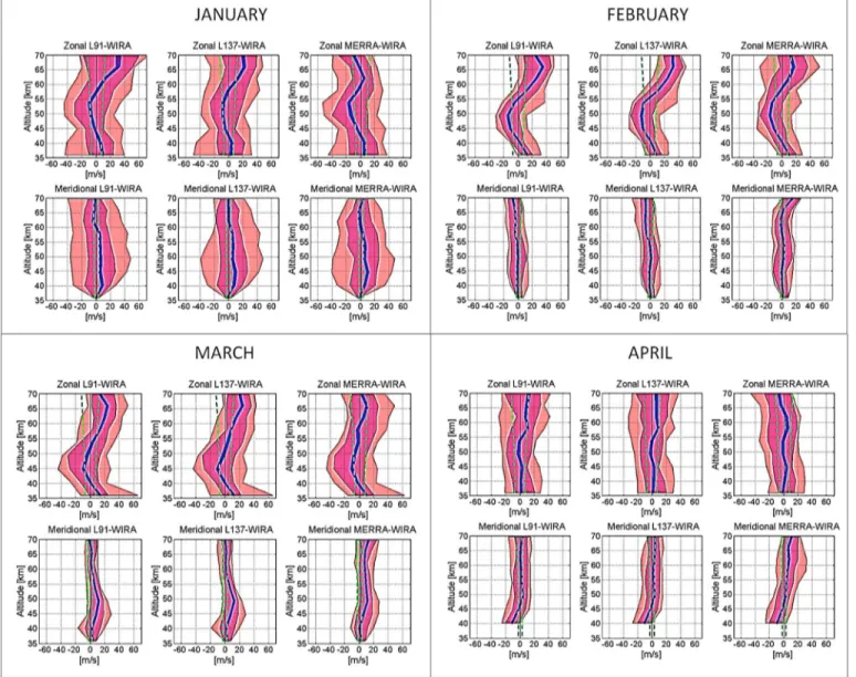
Figure 7 shows the monthly statistical distribution of the differences between zonal and meridional wind models and WIRA observations. Model data have been convolved with the averaging kernels of WIRA to

Figure 5. Comparison between the power spectral density (PSD) of the lidar data (blue) and model output (red) at 1 hPa (~48 km) over OHP. (a) ECMWF (reanalysis product ERA-Interim, 2003–2013). (b) MERRA (2003–2013). (c) MPI-ESM-LR (1991–2005), each line corresponds to one ensemble member.

(10)

account for the limited vertical grid of the instrument. As for the temperature (Figure 4), the median of the dif-ferences are overall in good agreement between 30 and 60 km. The standard deviation of the mean, especially above 60 km, falls outside of the instrumental error (green dashed lines, see Table S1) and thus can be consid-ered statistically signiﬁcant (larger than 20 m/s for the zonal wind). As for the temperature (see Figure 4), larger differences are noted during the winter months with a similar phase shifted pattern which is likely related to failure of the numerical models to resolve planetary wave one correctly (see section 3.1.1).

Figure S4 shows distributions considering the entire OHP campaign. From the zonal wind distribution for both L137 and MERRA, we estimate a mean negative difference of 10–15 m/s around 50 km. The standard error of the mean increases with altitude and reaches +20 m/s at 70 km. The 95% distribution ranges from about 40 m/s at 50 km and a maximum of +50 m/s at 65 km. For the meridional wind, a positive difference of ~10 m/s is noted in the deviation of the mean at 50 km. Between 35 and 70 km, the 95% distribution ranges from ~ 20 to ~30 m/s. Although ECMWF and MERRA exhibit comparable distributions in the difference, a larger variance is noted in the difference above 50 km for MERRA.

3.3. ECMWF Model Validation Using Continuous Infrasound Recordings

While lidar and microwave soundings provide vertical information above the station, infrasound signals are sensitive to the combined effects of refraction due to sound speed gradients and advection due to along-path wind on propagation. Figure 8 presents infrasound signals (in black) detected at OHP in the micro-barom band (0.1–0.3 Hz) from October 2012 to May 2013. The detected microbarom signals originate from the North Atlantic [e.g., Assink et al., 2014b]. The infrasound detections are superimposed on the effective sound speed ratio (Ceff-ratio) which is deﬁned as the ratio between the maximum of the along-path wind

plus the adiabatic sound speed at 30–60 km altitude and the sound speed at the ground level [see, for example, Le Pichon et al., 2012]. In the microbarom frequency band, C_eff-ratiocontrols to aﬁrst order the pressure attenuation, which combines the effects of both geometrical spreading and dissipation on the wave amplitude. This parameter is calculated using ECMWF (L91) wind and temperature products. Values of Ceff-ratiolarger than 1 (red regions) indicate favorable downwind propagation. Detections are

Figure 6. Comparison between daily averaged L91, L137, MERRA zonal wind products, and WIRA observations at OHP. Wind values are averaged between 30–40, 40–50, 50–60, and 60–70 km.

(11)

compared to predicted microbarom signals detectable above the background noise level at the station, that propagate through the stratospheric waveguide up to 50–55 km, by applying an empirically derived pressure wave attenuation relation [Le Pichon et al., 2012]. The predicted back azimuths (with respect to the OHP array) of microbarom signals (in green) are calculated using a source model developed by

Figure 8. Infrasound monitoring of microbaroms from North Atlantic at OHP. Detected (black dots) and predicted signals (green regions) superimposed on the color-coded Ceff-ratio(from L91) computed above OHP in the full range of azimuths. The red regions indicate favorable stratospheric propagation conditions,

while blue to white colors indicate that stratospheric propagation is unlikely.

Figure 7. Distribution of the monthly difference between ECMWF wind product at 12:00 UTC and daily averaged WIRA measurements versus altitude at OHP from January to April 2013. Blue lines: standard error of the mean. Green dashed lines: instrumental error bars. The differences are signiﬁcant when the blue lines fall outside of the green dashed lines. Purple and pink regions: 66% and 95% intervals obtained from the distribution of difference proﬁles.

(12)

Waxler and Gilbert [2006] and the sea state using the ECMWF two-dimensional wave energy spectrum ocean wave product [ECMWF, 2013].

During winter, the eastward circumpolar vortex favors long-range downwind propagation of signals from westerly directions. Improved detection capability occurs downwind from October 2012 to May 2013. While a general agreement between the observed and predicted microbarom azimuths is found, similar to earlier studies by Walker [2012] and Assink et al. [2014b], differences up to ~20° are often observed. These differences could be associated with approximations in long-range propagation modeling (azimuth uncor-rected for transversal wind effects and range-independent atmospheric profiles) [e.g., Walker, 2012; Assink et al., 2014b] as well as uncertainties in the wave parameter estimation [Szuberla and Olson, 2004]. During the onset of the SSW, we note an increased number of low-frequency signals (5–10 s period) from northeast-erly direction. These signals could be interpreted as Pacific microbarom signals or orographic waves from the Alps. Thefirst-order agreement is in accordance with the lidar and WIRA comparisons shown in Figures 2 and 7. Deviations from this trend (e.g., unpredicted signals under favorable propagation conditions and low background station noise or detected signals out of the expected range of azimuth) are either related to short time scale varia-bility of the atmosphere not represented in ECMWF analyses (e.g., inaccuracy in the modeled direction of the wind vector and strength) with resulting local differences in the large-scale circulation or can be explained by unre-solved changes in the nature of the microbarom sources. In a related study [Assink et al., 2014a], an evaluation of ECMWF analyses using volcanic signals has been performed. While afirst-order agreement was found, large discrepancies during the equinox periods were observed when the atmosphere is in a state of transition. The reported deviations of up to 30 m/s at 50 km altitude were found to be in line with our 95% distribution.

4. Discussion

Current research and development efforts are focused on the implementation of fully assimilative high-top global circulation models to quantify the coupling between the lower, middle, and upper atmosphere and ionosphere [e.g., Akmaev, 2011]. Operational weather and climate models provide 4-Dfields of meteorologi-cal variables up to ~80 km. In this study, collocated lidar, wind radiometer profiles as well as continuous infra-sound recordings are used to evaluate ECMWF analyses, MERRA reanalyses, and the MPI-ESM climate model output in the MA, where limited data assimilation occurs operationally. The presented results are essentially limited to comparisons between GCM stable representation and local wind and temperature sounding profiles. While part of the observed discrepancies could be associated with unresolved physics in the GCM, another part can be related to differences in spatial and temporal sampling. However, the presented statistics based on long time series of nightly averaged lidar and daily averaged WIRA data provide first-order estimates of similarities and differences depending on ranges of altitude and seasons, as well as information on atmospheric structures at temporal scales that GCM can resolve.

For both temperature and horizontal wind components, comparisons highlight differences increasing with altitude. Wefind that the modeled and observed temperatures and horizontal winds are in general agree-ment up to ~40 km, although significant small biases in both variables are noted, over a timespan of 6 months. Throughout the MA, the differences are characterized by broad distributions. Between 40 and 60 km altitude, the standard deviation of the mean difference exceeds 5 K for the temperature and 20 m/s for the zonal wind. In this range of altitude, the 95% distribution of the difference exceeds 30 K for the tem-perature and 40 m/s for the zonal wind. The largest deviations are observed in winter when the variability from large-scale planetary waves dominates over the general circulation. After the vernal equinox, the differ-ences reduce by about a factor 2. Compared to L91 model, L137 and MERRA models are in better agreement with lidar data above 60 km. Between 10 and 0.1 hPa, comparative spectral analyses confirm the lack of varia-bility on shorter time scales (up to 20 days and in the order of ~10 dB at 5 day period) that is neither present in ECMWF and MERRA products nor in the free-running MPI-ESM-LR climate model. These results are in line with a recent study by Hoppel et al. [2013], who showed that assimilation of microwave imager/sounder data could provide reliable large-scale constraints throughout the mesosphere for operational high-altitude analysis. Combined with lidar and wind radiometer observations, infrasound measurements provide additional integrated information about the structure of the stratosphere where data coverage is sparse. The observed infrasound parameters from microbaroms are overall in agreement with the simulated values, which is consistent with the lidar and WIRA observations. However, on shorter time scales, deviations in the detected

(13)

source intensity and direction are consistent with the lack of variability found in both temperature and wind models. More analyses like the one presented here will better determine the role of different factors that inﬂuence propagation predictions and could infer more precisely atmospheric corrections by including additional infrasonic observables (such as the wave amplitude and period). In particular, improvements of the microbarom predictions would require more accurate source and propagation models [e.g., Landès et al., 2014]. With the increasing number of IMS and other infrasonic arrays deployed around the globe, more systematic studies using historical infrasound data set and state-of-the-art reanalysis systems could provide useful information on the polar vortex structure and the longer-term inﬂuences of SSWs on the troposphere [e.g., Charlton-Perez et al., 2007; Mitchell et al., 2013; Smets and Evers, 2014].

5. Conclusions

The validation of the analysis products in the lower and middle atmosphere is relevant to a broad community and for a wide variety of applications. Simulating realistic MA variability and reducing biases remain a chal-lenge for all climate models [e.g., Sigmond and Scinocca, 2010; Hardiman et al., 2012]. Furthermore, the lack of stratospheric variability in the low-top models has an impact on stratosphere-troposphere coupling which do not produce long-lasting tropospheric impacts as seen in observations [e.g., Charlton-Perez et al., 2013]. Recent studies have demonstrated that dynamics in the stratosphere play a signiﬁcant role in tropospheric weather [e.g., Sigmond et al., 2013]. Thus, correctly predicting the evolution of atmospheric extreme events like SSWs can lead to improvements in tropospheric weather forecasts on weekly time scales [e.g., Tripathi et al., 2014].

This study demonstrates the advantage of an infrastructure that integrates various independent middle atmospheric measurement techniques currently not assimilated in NWP models and provides quantitative understanding of stratosphere-troposphere dynamical coupling useful for NWP applications. It can be antici-pated that continuing such investigations could be of considerable value for NWP applications, as climate science including monthly and seasonal predictability requires an improved quantitative understanding of the dynamical coupling between the MA and the troposphere.

Beyond the atmospheric community, the evaluation of NWP models is essential in the context of the future ver-ification of the CTBT as improved atmospheric models are extremely helpful to assess the IMS network perfor-mance in higher resolution, reduce source location errors, and characterization methods. Capitalizing on such scientific and technical advances should reinforce the potential benefit of a routine and global use of infra-sound for civil applications and enlarge the science community interested by operational infrainfra-sound monitor-ing. In particular, infrasound has proven to be extremely efficient in providing reliable source information on active volcanoes from local to long-range (thousands of kilometers) observations [e.g., Dabrowa et al., 2011; Tailpied et al., 2013; Matoza et al., 2011]. For this typical application, the use of improved atmospheric speci fica-tions will allow for reliable confidence level estimates associated with remote volcanic hazard assessments.

References

Akmaev, R. A. (2011), Whole atmosphere modeling: Connecting terrestrial and space weather, Rev. Geophys., 49, RG4004, doi:10.1029/ 2011RG000364.

Angot, G., P. Keckhut, A. Hauchecorne, and C. Claud (2012), Contribution of stratospheric warmings to temperature trends in the middle atmosphere from the lidar series obtained at Haute-Provence Observatory (44°N), J. Geophys. Res., 117, D21102, doi:10.1029/2012JD017631. Assink, J. D., A. Le Pichon, E. Blanc, M. Kallel, and L. Khemiri (2014a), Evaluation of wind and temperature proﬁles from ECMWF analysis on two

hemispheres using volcanic infrasound, J. Geophys Res. Atmos., 119, 8659–8683, doi:10.1002/2014JD021632.

Assink, J. D., R. Waxler, P. Smets, and L. G. Evers (2014b), Bi-directional infrasonic ducts associated with sudden stratospheric warming events, J. Geophys. Res. Atmos., 119, 1140–1153, doi:10.1002/2013JD021062.

Baldwin, M. P., D. W. J. Thompson, E. F. Shuckburgh, W. A. Norton, and N. P. Gillett (2003), Weather from the stratosphere?, Science, 301, 317–319, doi:10.1126/science.1085688.

Baron, P., et al. (2013), Observation of horizontal winds in the middle-atmosphere between 30°S and 55°N during the northern winter 2009–2010, Atmos. Chem. Phys., 13, 6049–6064, doi:10.5194/acpd-12-32473-2012.

Blanc, E., T. Farges, A. Le Pichon, and P. Heinrich (2014), Ten year observations of gravity waves from thunderstorms in western Africa, J. Geophys. Res. Atmos., 119, 6409–6418, doi:10.1002/2013JD020499.

Charlton-Perez, A. J., A. O’Neill, W. A. Lahoz, and A. C. Massacand (2004), Sensitivity of tropospheric forecasts to stratospheric initial conditions, Q. J. R. Meteorol. Soc., 130, 1771–1792, doi:10.1256/qj.03.167.

Charlton-Perez, A. J., L. M. Polvani, J. Perlwitz, F. Sassi, E. Manzini, K. Shibata, S. Pawson, J. E. Nielsen, and D. Rind (2007), A new look at stratospheric sudden warmings. Part II: Evaluation of numerical model simulations, J. Clim., 10, 470–488, doi:10.1175/JCLI3994.1. Charlton-Perez, A. J., et al. (2013), On the lack of stratospheric dynamical variability in low-top versions of the CMIP5 models, J. Geophys. Res.

Atmos., 118, 2494–2505, doi:10.1002/jgrd.50125.

Acknowledgments

This work was partly performed during the course of the ARISE design study project, funded by the Seventh Framework Program (FP7) of the European Union (grant 284387), that aims to design a novel infrastructure by integrating new type of high-resolution MA observation networks. The data presented in this paper are available through the ARISE prototype data portal (accessible via the project website http://arise-project.eu). We thank the infrasound station operators at CEA (Ph. Millier, F. Tinel, and J.M. Koenig), the research group at OHP (J.M. Perrin) for hosting the infrasound experimental array and operating the Rayleigh lidar equipment, and Th. Leblanc for guaranteeing the long-term high-quality lidar measurements at Table Mountain facility which contribute to the NDACC database. D.P. Drob acknowledges support from the Chief of Naval Research, Naval Research Laboratory 6.1 base research program. The authors are also grateful to Pr. Adrian Simmons (ECMWF) for his interest in this study and helpful comments. Some of the data used in this publication were obtained as part of the Network for the Detection of Atmospheric Composition Change (NDACC) and are publicly available (accessible via http://www.ndacc.org). The NASA MERRA data used in this study have been provided by the Global Modeling and Assimilation Ofﬁce at NASA Goddard Space Flight Center through the NASA GES DISC online archive (http://gmao.gsfc.nasa.gov/ products/).

(14)

Chunchuzov, I. P., S. N. Kulichkov, and P. P. Firstov (2013), On acoustic N-wave reﬂections from atmospheric layered inhomogeneities, Izv. Atmos. Oceanic Phys., 49(3), 285–297.

Coy, L., S. D. Eckermann, K. W. Hoppel, and F. Sassi (2011), Mesospheric precursors to the major stratospheric sudden warming of 2009: Validation and dynamical attribution using a ground-to-edge-of-space data assimilation system, J. Adv. Model. Earth Syst., 3, M10002, doi:10.1029/2011MS000067.

Dabrowa, A. L., D. N. Green, A. C. Rust, and J. C. Phillips (2011), A global study of volcanic infrasound characteristics and the potential for long-range monitoring, Earth and Planet. Sci. Lett., 310, 369–379, doi:10.1016/j.epsl.2011.08.027.

Dee, D. P. (2005), Bias and data assimilation, Q. J. R. Meteorol. Soc., 131, 3323–3343, doi:10.1256/qj.05.137.

Derber, J. C., and W. S. Wu (1998), The use of TOVS cloud-cleared radiances in the NCEP SSI analysis system, Mon. Weather Rev., 126, 2287–2299. Diamantakis, M. (2014), Improving ECMWF forecasts of sudden stratospheric warmings. ECMWF Newsletter, 141, October 2014. Drob, D. P., R. R. Meier, J. M. Picone, and M. Garcés (2010), Inversion of infrasound signals for passive atmospheric remote sensing, in

Infrasound Monitoring for Atmospheric Studies, edited by A. Le Pichon, E. Blanc, and A. Hauchecorne, chap. 24, pp. 701–732, Springer, New York.

ECMWF (2013), IFS documentation Cy38r1. Operational implementation 19 June 2012, Tech. Rep., European Centre for Medium-Range Weather Forecasts, Reading, U. K.

Evers, L. G., and P. Siegmund (2009), Infrasonic signature of the 2009 major sudden stratospheric warming, Geophys. Res. Lett, 36, L23808, doi:10.1029/2009GL041323.

Hamilton, K. (1991), Climatological statistics of stratospheric inertia-gravity waves deduced from historical rocketsonde wind and tem-perature data, J. Geophys. Res., 96, 20,831–20,839, doi:10.1029/91JD02188.

Hardiman, S. C., N. Butchart, T. J. Hinton, S. M. Osprey, and L. J. Gray (2012), The effect of a well resolved stratosphere on surface climate: Differences between CMIP5 simulations with high and low top versions of the Met Ofﬁce climate model, protect, J. Clim., 25, 7083–7099, doi:10.1175/JCLI-D-11-00579.1.

Hays, P. B., V. J. Abreu, M. E. Dobbs, D. A. Gell, H. J. Grassl, and W. R. Skinner (1993), The high-resolution Doppler imager on the Upper Atmosphere Research Satellite, J. Geophys. Res., 98, 10,713–10,723, doi:10.1029/93JD00409.

Hoppel, K. W., S. D. Eckermann, L. Coy, G. E. Nedoluha, D. R. Allen, S. D. Swadley, and N. L. Baker (2013), Evaluation of SSMIS upper atmosphere sounding channels for high-altitude data assimilation, Mon. Weather Rev., 141, 3314–3330, doi:10.1175/mwr-d-13-00003.1.

Keckhut, P., A. Hauchecorne, and M. L. Chanin (1993), A critical review of the database acquired for the long-term surveillance of the middle atmosphere by the French Rayleigh lidars, J. Atmos. Oceanic Technol., 10, 850–867, doi:10.1175/1520-0426(1993)010<0850: ACROTD>2.0.CO;2.

Khaykin, S. M., A. Hauchecorne, N. Mze, and P. Keckhut (2015), Seasonal variation of gravity wave activity at mid-latitudes from 7 years of COSMIC GPS and Rayleigh lidar temperature observations, Geophys. Res. Lett., 42, 1251–1258, doi:10.1002/2014GL062891.

Kishore Kumar, G., K. Kishore Kumar, W. Singer, C. Zülicke, S. Gurubaran, G. Baumgarten, G. Ramkumar, S. Sathishkumar, and M. Rapp (2014), Mesosphere and lower thermosphere zonal wind variations over low latitudes: Relation to local stratospheric zonal winds and global circulation anomalies, J. Geophys. Res. Atmos., 119, 5913–5927, doi:10.1002/2014JD021610.

Kulichkov, S. (2010), On the prospect for acoustic sounding of theﬁne structure of the middle-atmosphere, in Infrasound Monitoring for Atmospheric Studies, edited by A. Le Pichon, E. Blanc, and A. Hauchecorne, pp. 511–540, Springer, Dordrecht, New York.

Lalande, J.-M., O. Sèbe, M. Landès, P. Blanc-Benon, R. Matoza, A. L. Pichon, and E. Blanc (2012), Infrasound data inversion for atmospheric sounding, Geophys. J. Int., 190, 687–701, doi:10.1111/j.1365-246X.2012.05518.x.

Landès, M., N. Shapiro, A. Le Pichon, G. Hillers, and M. Campillo (2014), Explaining global patterns of microbarom observations with wave action models, Geophys. J. Int., 199, 1328–1337, doi:10.1093/gji/ggu324.

Laštovička, J., G. Beig, and D. R. Marsh (2014), Response of the mesosphere-thermosphere-ionosphere system to global change: CAWSES-II contribution, Prog. Earth Planet. Sci., 1, 21, doi:10.1186/s40645-014-0021-6.

Le Pichon, A., L. Ceranna, and J. Vergoz (2012), Incorporating numerical modeling into estimates of the detection capability of the IMS infrasound network, J. Geophys. Res., 117, D05121, doi:10.1029/2011JD0166702009.

Liu, H.-L., V. A. Yudin, and R. G. Roble (2013), Day-to-day ionospheric variability due to lower atmosphere perturbations, Geophys. Res. Lett., 40, 665–670, doi:10.1002/grl.50125.

Long, D. J., D. R. Jackson, J. Thuburn, and C. Mathison (2013), Validation of Met Ofﬁce upper stratospheric and mesospheric analyses, Q. J. R. Meteorol. Soc., 139, 1214–1228, doi:10.1002/qj.2031.

Manney, G. L., et al. (2008), The evolution of the stratopause during the 2006 major warming: Satellite data and assimilated meteorological analyses, J. Geophys. Res., 113, D11115, doi:10.1029/2007JD009097.

Matoza, R. S., A. Le Pichon, J. Vergoz, P. Herry, J. M. Lalande, H. Lee, I. Y. Che, and A. Rybin (2011), Infrasonic observations of the June 2009 Sarychev Peak eruption, Kuril Islands: Implications for infrasonic monitoring of remote explosive volcanism, J. Volcanol. Geotherm. Res., doi:10.1016/j.jvolgeores.2010.11.022.

Mitchell, D. M., J. Lesley, J. Anstey, M. Baldwin, and A. J. Charlton-Perez (2013), The inﬂuence of stratospheric vortex displacements and splits on surface climate, J. Clim., 26, 2668–2682, doi:10.1175/JCLI-D-12-00030.1.

Nielsen, K., D. E. Siskind, S. D. Eckermann, K. W. Hoppel, L. Coy, J. P. McCormack, S. Benze, C. E. Randall, and M. E. Hervig (2010), Seasonal variation of the quasi 5 day planetary wave: Causes and consequences for polar mesospheric cloud variability in 2007, J. Geophys. Res., 115, D18111, doi:10.1029/2009JD012676.

Pawson, S., et al. (2000), The GCM-Reality Intercomparison Project for SPARC (GRIPS): Scientiﬁc issues and initial results, Bull. Am. Meteorol. Soc., 81, 781–796, doi:10.1175/1520-0477(2000)081<0781:TGIPFS>2.3.CO;2.

Podglajen, A., A. Hertzog, R. Plougonven, and N.Žagar (2014), Assessment of the accuracy of (re)analyses in the equatorial lower stratosphere, J. Geophys. Res. Atmos., 119, 11,166–11,188, doi:10.1002/2014JD021849.

Polavarapu, S., T. G. Shepherd, Y. Rochon, and S. Ren (2005), Some challenges of middle atmosphere data assimilation, Q. J. R. Meteorol. Soc., 131, 3513–3527, doi:10.1256/qj.05.87.

Press, W. H., S. A. Teukolsky, S. T. Vetterling, and B. P. Flannery (1994), Numerical Recipes in C: The Art of Scientiﬁc Computing, 2nd ed., 994 pp., Cambridge Univ. Press, Cambridge.

Randel, W., et al. (2004), The SPARC intercomparison of middle-atmosphere climatologies, J. Clim., 17, 986–1003, doi:10.1175/1520-0442 (2004)017<0986:TSIOMC>2.0.CO;2.

Rienecker, M. M., et al. (2011), MERRA: NASA’s Modern-Era Retrospective Analysis for Research and Applications, J. Clim., 24, 3624–3648, doi:10.1175/JCLI-D-11-00015.1.

Rüfenacht, R., N. Kämpfer, and A. Murk (2012), First middle-atmospheric zonal wind proﬁle measurements with a new ground-based microwave Doppler-spectro-radiometer, Atmos. Meas. Tech., 5, 2647–2659, doi:10.5194/amt-5-2647-2012.

(15)

Rüfenacht, R., A. Murk, N. Kämpfer, P. Eriksson, and S. A. Buehler (2014), Middle-atmospheric zonal and meridional wind proﬁles from polar, tropical and mid-latitudes with the ground-based microwave Doppler wind radiometer WIRA, Atmos. Meas. Tech., 7, 4491–4505, doi:10.5194/amt-7-4491-2014.

Russell, J. M., M. G. Mlynczak, L. L. Gordley, J. J. Tansock, and R. W. Esplin (1999), An overview of the SABER experiment and preliminary calibration results, Proc. SPIE Int. Soc. Opt. Eng., 3756, 277–288.

Sakazaki, T., M. Fujiwara, X. Zhang, M. E. Hagan, and J. M. Forbes (2012), Diurnal tides from the troposphere to the lower mesosphere as deduced from TIMED/SABER satellite data and six global reanalysis data sets, J. Geophys. Res., 117, D13108, doi:10.1029/2011JD017117. Sigmond, M., and J. F. Scinocca (2010), The inﬂuence of the basic state on the Northern Hemisphere circulation response to climate change,

J. Clim., 23, 1434–1446, doi:10.1175/2009JCLI3167.1.

Sigmond, M., J. F. Scinocca, V. V. Kharin, and T. G. Shepherd (2013), Enhanced seasonal forecast skill following stratospheric sudden warmings, Nat. Geosci., 6, 98–102, doi:10.1038/ngeo1698.

Siskind, D. E., D. P. Drob, K. F. Dymond, and J. P. McCormack (2014), Simulations of the effects of vertical transport on the thermosphere and ionosphere using two coupled models, J. Geophys. Res. Space Physics, 119, 1172–1185, doi:10.1002/2013JA019116.

Smets, P. S. M., and L. G. Evers (2014), The life cycle of a sudden stratospheric warming from infrasonic ambient noise observations, J. Geophys. Res. Atmos., 119, doi:10.1002/2014JD021905.

Smith, A. K. (2003), The origin of stationary planetary waves in the upper mesosphere, J. Atmos. Sci., 60, 3033–3041, doi:10.1175/1520-0469 (2003)060<3033:TOOSPW>2.0.CO;2.

Smith, S. A., and D. C. Fritts (1984), Poker Flat MST radar and meteorological rocketsonde wind proﬁle comparisons, Geophys. Res. Lett., 11, 538–540, doi:10.1029/GL011i005p00538.

Swinbank, R., and D. A. Ortland (2003), Compilation of wind data for the Upper Atmosphere Research Satellite (UARS) reference atmosphere project, J. Geophys. Res., 108(D19), 4615, doi:10.1029/2002JD003135.

Szuberla, C. A. L., and J. V. Olson (2004), Uncertainties associated with parameter estimation in atmospheric infrasound arrays, J. Acoust. Soc. Am., 115, 253–258, doi:10.1121/1.1635407.

Tailpied, D., A. Le Pichon, E. Marchetti, M. Ripepe, M. Kallel, L. Ceranna, and N. Brachet (2013), Remote infrasound monitoring of Mount Etna: Observed and predicted network detection capability, InfraMatics, 2, doi:10.4236/inframatics.2013.21001.

Tripathi, O. P., et al. (2014), The predictability of the extratropical stratosphere on monthly time-scales and its impact on the skill of tropospheric forecasts, Q. J. R. Meteorol. Soc, 141, 987–1003, doi:10.1002/qj.2432.

Walker, K. (2012), Evaluating the opposing wave interaction hypothesis for the generation of microbaroms in the eastern North Paciﬁc, J. Geophys. Res., 117, C12016, doi:10.1029/2012JC008409.

Waxler, R., and K. E. Gilbert (2006), The radiation of atmospheric microbaroms by ocean waves, J. Acoust. Soc. Am., 119(5), 2651–2664. Wendt, V., S. Wust, M. G. Mlynczak, J. M. Russell, J. H. Yee, and M. Bittner (2013), Impact of atmospheric variability on validation of