HAL Id: hal-00302281
https://hal.archives-ouvertes.fr/hal-00302281
Submitted on 25 Feb 2004
HAL is a multi-disciplinary open access
archive for the deposit and dissemination of
sci-entific research documents, whether they are
pub-lished or not. The documents may come from
teaching and research institutions in France or
abroad, or from public or private research centers.
L’archive ouverte pluridisciplinaire HAL, est
destinée au dépôt et à la diffusion de documents
scientifiques de niveau recherche, publiés ou non,
émanant des établissements d’enseignement et de
recherche français ou étrangers, des laboratoires
publics ou privés.
forced by periodic wind stress
B. T. Kuebel Cervantes, J. S. Allen, R. M. Samelson
To cite this version:
B. T. Kuebel Cervantes, J. S. Allen, R. M. Samelson. Lagrangian characteristics of continental shelf
flows forced by periodic wind stress. Nonlinear Processes in Geophysics, European Geosciences Union
(EGU), 2004, 11 (1), pp.3-16. �hal-00302281�
SRef-ID: 1607-7946/npg/2004-11-3
Nonlinear Processes
in Geophysics
© European Geosciences Union 2004
Lagrangian characteristics of continental shelf flows forced by
periodic wind stress
B. T. Kuebel Cervantes, J. S. Allen, and R. M. Samelson
College of Oceanic and Atmospheric Sciences, Oregon State Univ., 104 Ocean Admin. Bldg., Corvallis, OR, 97 331, USA Received: 18 June 2003 – Revised: 3 November 2003 – Accepted: 4 November 2003 – Published: 25 February 2004 Part of Special Issue “Dedicated to Prof. A. D. Kirwan Jr. on the occasion of his 70th birthday”
Abstract. The coastal ocean may experience periods of fluc-tuating along-shelf wind direction, causing shifts between upwelling and downwelling conditions with responses that are not symmetric. We seek to understand these asymmetries and their implications on the Eulerian and Lagrangian flows. We use a two-dimensional (variations across-shelf and with depth; uniformity along-shelf) primitive equation numerical model to study shelf flows in the presence of periodic, zero-mean wind stress forcing. The model bathymetry and initial stratification is typical of the broad, shallow shelf off Duck, NC during summer. After an initial transient adjustment, the response of the Eulerian fields is nearly periodic. Despite the symmetric wind stress forcing, there exist both mean Eule-rian and Lagrangian flows. The mean Lagrangian displace-ment of parcels on the shelf depends both on their initial lo-cation and on the initial phase of the forcing. Eulerian mean velocities, in contrast, have almost no dependence on initial phase. In an experiment with sinusoidal wind stress forc-ing of maximum amplitude 0.1 N m−2and period of 6 days, the mean Lagrangian across-shelf displacements are largest in the surface and bottom boundary layers. Parcels that orig-inate near the coast in the top 15 m experience complicated across-shelf and vertical motion that does not display a clear pattern. Offshore of this region in the top 10 m a rotating cell feature exists with offshore displacement near the surface and onshore displacement below. A mapping technique is used to help identify the qualitative characteristics of the Lagrangian motion and to clarify the long time nature of the parcel dis-placements. The complexity of the Lagrangian motion in a region near the coast and the existence of a clear boundary separating this region from a more regular surface cell fea-ture offshore are quantified by a calculation from the map of the largest Lyapunov exponent.
Correspondence to: B. T. Kuebel Cervantes ([email protected])
1 Introduction
In this study we examine the Lagrangian characteristics of two-dimensional, time-periodic, wind-driven coastal flows. The wind-driven processes of upwelling and downwelling are of considerable interest to coastal oceanographers study-ing the physics and biology of these highly productive re-gions. Most modeling studies of coastal flows have been an-alyzed in terms of a traditional Eulerian formulation. The Lagrangian aspects of these flows typically have not been considered. A description of the Lagrangian behaviour of wind-driven shelf flow has recently been pursued by Kuebel Cervantes et al. (2003), hereafter denoted as KC2003, which motivated this work. The study by KC2003 utilized numer-ical experiments to examine the Eulerian and Lagrangian characteristics of wind-driven coastal upwelling and down-welling forced by measured winds at Duck, North Carolina during the Coastal Ocean Processes (CoOP) Inner Shelf Study (ISS). The ISS took place off Duck from August– November 1994. Interesting Lagrangian behaviour was found during the month of August that resulted from the varying along-shelf wind stress direction. The present study further investigates the impact of the fluctuating along-shelf winds on fluid parcels in the coastal ocean using periodic wind forcing with zero time mean. We use a Lagrangian parcel tracking technique to study fluid parcel displacements over one period and many periods, as well as to compute mean Lagrangian velocities. We also employ a technique utilized by KC2003 of advecting Lagrangian label fields by the model velocities for further Lagrangian analyses.
Eulerian dynamics are discussed as well. The Eulerian fields are approximately periodic after an initial adjustment of a few periods. Although the forcing is periodic, mean Eulerian velocities exist after one period. Asymmetries be-tween upwelling and downwelling, including the thickness of the surface and bottom mixed layers and the relative im-portance of nonlinear advection, were discussed by KC2003 and are revisited here.
8T 8.25T 8.5T 8.75T 9T 9.25T 9.5T −0.1 −0.05 0 0.05 0.1 τ sy (N m − 2 )
Fig. 1. Sinusoidal along-shelf wind stress forcing for a portion of
the spinup run duration (shown after 8 periods). The dotted lines show the times in the forcing period at which model simulations with ti=8.5 T, ti=8.75 T, ti=9 T, and ti=9.25 T are initialized.
0 T 2T 3T 4T 5T 6T 7T 8T 9T −0.2 −0.1 0 0.1 0.2 V (m s − 1)
Fig. 2. Depth-averaged along-shelf velocity at 8 m depth
(approxi-mately 2.7 km from the coast) for a 9-period spinup run.
The present investigation has relevance to two differ-ent scidiffer-entific communities: coastal oceanography and dy-namical systems. While these fields are traditionally un-related, studies in recent years have bridged the gap be-tween the two fields through the application of dynamical systems techniques to oceanographic flows. Ridderinkhof and Loder (1994) and Loder et al. (1997) identify hyper-bolic fixed points and their associated stable and unstable manifolds in tidal flows over submarine banks. More re-cently, Poje et al. (2002) use an ocean model to determine optimal Lagrangian drifter launch sites by tracking hyper-bolic points in the flow field and Kirwan et al. (2003) ap-ply ideas of invariant manifolds to flow in the Gulf of Mex-ico using a data assimilating model. Early work combin-ing fluid mechanics and dynamical systems, such as that of Weiss and Knobloch (1989) and Rom-Kedar et al. (1990), consider transport properties of fluid in modulated travel-ing waves and unsteady vortical flow, respectively. Many studies from the dynamical systems perspective, including Coulliette and Wiggins (2001), Miller et al. (1997), and Poje and Haller (1999), apply dynamical systems theory to study lobe geometry and dynamics and invariant manifolds in ve-locity fields from ocean circulation models. Most recently, these techniques have also been developed for application to two-dimensional time-dependent ocean velocity measure-ments (Ide et al., 2002 and Haller, 2002). These examples indicate that the study of oceanic flows using dynamical sys-tems methods is clearly of interest to oceanographers and ap-plied mathematicians, however coastal ocean flows over the continental shelf have generally not been the focus of these studies.
The outline of the paper is as follows. The numeri-cal model methods and particle tracking techniques are de-scribed in Sect. 2. The dynamical analysis of the Eulerian mean velocity and momentum balance fields is discussed in Sect. 3. The Lagrangian results are presented in Sect. 4. A summary is given in Sect. 5.
2 Methods
2.1 Model description
The numerical model is a two-dimensional version of the finite-difference Princeton Ocean Model (POM) (Blumberg and Mellor, 1987). The model equations are the hydrostatic primitive equations with the Mellor-Yamada (1982) turbu-lence closure scheme for vertical mixing, as modified in Galperin et al. (1988), embedded.
The model domain, described in terms of Cartesian coordi-nates (x, y, z), is a section with variations in the across-shelf (x) and vertical (z) directions. The flow is assumed to be uniform in the along-shelf (y) direction, so that the Eulerian variables have no y dependence. The velocity components in the (x, y, z) directions are (u, v, w). Note that although the flow is uniform in y, the along-shelf velocity component v is generally not zero. The domain is bounded by vertical walls at the coast and at the offshore boundary with boundary con-ditions of no flow in the across-shelf direction (u = 0) and free-slip in the along-shelf direction (vx=0).
For application over variable bottom topography, the POM model is formulated in sigma coordinates (x, y, σ ). The re-lationship between σ and the Cartesian vertical coordinate z is given by
σ = z − η
H + η, (1)
where D=H + η, H (x) is the depth and η(x, t ) is the surface elevation, so that σ = 0 at the surface (z=η) and σ = − 1 at the bottom (z= − H ). Consequently, when discretized, the same number of σ levels exist independent of the local depth and the vertical resolution increases as the depth decreases. In σ coordinates, ω is a velocity normal to σ surfaces that en-ters the equations naturally and replaces the vertical velocity
w. The relationship between ω and w is
ω = w − u(σ∂D ∂x + ∂η ∂x) − σ ∂D ∂t − ∂η ∂t. (2)
In the analysis of model solutions, we present the results in terms of the original Cartesian coordinates to facilitate phys-ical interpretation.
2.2 Model Setup
The model bathymetry, initial stratification, and forcing cor-respond to August conditions observed at Duck during the ISS. The initial state of the model experiments is a coastal ocean at rest with horizontally uniform temperature and salinity fields compiled from the horizontal average of those
0 10 20 30 40 50 0 10 20 30
9.25T
U (m s
−1
)
0 10 20 30 40 50 0 10 20 309.5T
0 10 20 30 40 50 0 10 20 309.75T
0 10 20 30 40 50 0 10 20 3010T
−0.1 −0.05 0 0.05 0.1 0 10 20 30 40 50 0 10 20 3010.25T
0 10 20 30 40 50 0 10 20 30V (m s
−1
)
0 10 20 30 40 50 0 10 20 30 0 10 20 30 40 50 0 10 20 30 0 10 20 30 40 50 0 10 20 30 −0.25 −0.125 0 0.125 0.25 0 10 20 30 40 50 0 10 20 30 0 10 20 30 40 50 0 10 20 30σ
θ
(kg m
−3
)
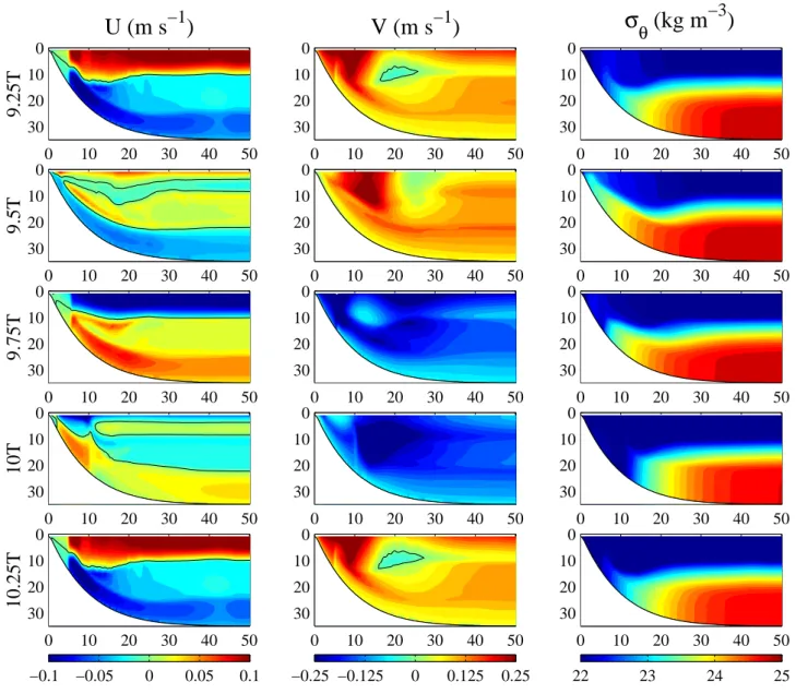
0 10 20 30 40 50 0 10 20 30 0 10 20 30 40 50 0 10 20 30 0 10 20 30 40 50 0 10 20 30 22 23 24 25 0 10 20 30 40 50 0 10 20 30Fig. 3. Eulerian across-shelf velocity u, along-shelf velocity v, and potential density σθduring one period beginning at ti=9.25 T. The black
line denotes the 0 contour for u and v.
observed with an across-shelf mooring array at Duck on 7 August 1994. The model is forced by a sinusoidal, spa-tially independent along-shelf wind stress component τsy and by constant heat flux components (shortwave radiative heat flux, Qsw, and the sum of the longwave and turbulent
fluxes, Qlw+Qsen+Qlat) computed from the mean heat flux
values observed at Duck in August (Austin and Lentz, 1999). The period of τsy is chosen to be 6 days based on the ap-proximate period of maximum wind-forced energy observed during August. The maximum amplitude of τsy, 0.1 N m−2,
is also typical of August values.
The model bathymetry is characteristic of that off Duck with a relatively steep slope from the coast to about 20 m depth and a gradual slope offshore of the 20 m isobath. The model domain extends from the coastal boundary to a dis-tance of 200 km offshore, with constant water depth of 35 m
offshore of 40 km. A uniform grid spacing is used in x with a resolution of 250 m and in σ with 30 σ levels. The hor-izontal kinematic eddy viscosity and diffusivity are chosen to be small constant values, AM=AH=2 m2s−1. The
back-ground vertical viscosity νM and diffusivity νH are set to
2.0×10⁻⁵m2s−1. The model has both an “external” time step to integrate the barotropic (depth-integrated) momen-tum equations and an “internal” time step to integrate the baroclinic (depth-dependent) momentum equations. The ex-ternal time step is 5 s and is governed by fast surface waves, whereas the internal time step is much longer, 75 s, because the baroclinic response is governed by slower internal waves. The model is spun up for several forcing periods after which the Eulerian fields are nearly periodic. In Sect. 4.2, we present results for parcels initialized at different phases in the forcing period. The net parcel displacements and Lagrangian
0 1T 2T 3T 4T 5T 6T 7T 8T 9T 10T −0.1 −0.05 0 0.05 0.1 τ sy (N m − 2 ) 0 1T 2T 3T 4T 5T 6T 7T 8T 9T 10T −0.18 −0.12 −0.060 0.06 0.12 0.18 v (m s − 1 ) − 0 1T 2T 3T 4T 5T 6T 7T 8T 9T 10T 0 0.01 0.02 0.03 0.04 0.05 v 2 (m 2 s − 2 )
_
−1 −0.5 0 0.5 1 0 0.5 1 1.5 2 2.5 ∂(KE)/∂t (10−3 m2 s−3) KE (10 − 2 m 2 s − 2 )__
__
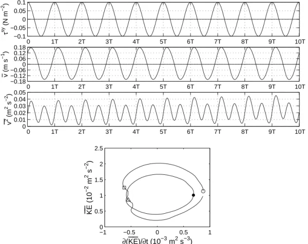
Fig. 4. Top three panels are time series of along-shelf wind stress (top), averaged along-shelf velocity (Eq. 3) (middle), and
area-averaged along-shelf velocity squared (bottom) during a 10-period simulation beginning at ti=9.25 T. Bottom panel is the area-averaged kinetic energyKE¯ (Eq. 4) vs. the time derivative ∂KE/∂t for the first period during the same simulation. The symbols in the bottom right plot correspond to ti=9.25 T (open circle), ti+T/4 (square), ti+T/2 (filled circle), and ti+3T/4 (triangle).
mean velocities over one period are highly sensitive to this initial phase. Results from the model simulations are refer-enced according to the start time, ti, given as the number of
periods in the long spinup run. Results will be presented for four different initialization times; ti=8.5 T, ti=8.75 T, ti=9 T, and ti=9.25 T (Fig. 1). Most of the results will focus
on the simulation beginning at ti=9.25 T, at which time the
wind forcing is in the middle of an upwelling-favorable half-cycle and the amplitude is maximum. The near periodicity of the Eulerian fields after several forcing periods is illustrated by the time-dependence of the depth-averaged along-shelf velocity in 8 m water depth during a 9-period spinup run in Fig. 2. The density values (not shown) decrease slightly with each period due to positive surface heat flux forcing, however the vertical gradient in density remains nearly periodic.
Contour plots of the Eulerian across-shelf velocity u, along-shelf velocity v, and potential density σθduring a
sim-ulation beginning at ti=9.25 T show the evolution of the
model fields over a forcing period (Fig. 3). The upwelling response of u with offshore flow in the surface and onshore flow in the bottom boundary layers is apparent initially at 9.25 T. The v field shows a northward coastal upwelling jet and σθshows most of the isopycnals intersect the bottom and
a few intersect the surface. The across-shelf flow then weak-ens and shifts to downwelling with surface onshore flow and offshore flow in the bottom layer at 9.75 T. The u field at 9.75 T is not equal and opposite that at 9.25 T, but is char-acterized by a slightly thinner surface layer from 10–20 km offshore and a more structured flow below the surface layer inshore of 20 km. Differences in the structure of u dur-ing transition between upwelldur-ing and downwelldur-ing condi-tions are seen at 9.5 T and 10 T. The along-shelf velocity changes rather suddenly from northward at 9.5 T to south-ward at 9.75 T. The isopycnals are upwelled along the bot-tom at 9.5 T and then move back down the shelf at 9.75 T. After 9.75 T, the across-shelf flow weakens again and returns to the upwelling response at 10.25 T. The along-shelf veloc-ity also becomes dominantly northward once again and the isopycnals return to their initial location at 9.25 T.
Time series of the Eulerian fields during a 10-period simu-lation beginning at ti=9.25 T further illustrate the nearly
pe-riodic nature of the flow (Fig. 4). The area-averaged along-shelf velocity, defined as
v = 1 A Z xb 0 Z η −H vdxdz, (3)
where A is the cross sectional area of the model domain, fol-lows the sinusoidal wind forcing with a lag of about 19 h, which is approximately the inertial period 2π/f . A slight increase in the maximum magnitude of v during upwelling forcing relative to downwelling forcing is seen. This differ-ence magnifies when v is squared (third panel); v2 is
sig-nificantly higher during upwelling than during downwelling. The plot of v2also reveals more clearly than the plot of v that
the periodicity is only approximate.
A phase-plane diagram of the area-averaged kinetic energy
KE versus the time derivative of kinetic energy ∂KE/∂t (Fig. 4, bottom panel) shows the difference in upwelling and downwelling energy responses. The area-averaged kinetic energy is calculated as KE = 1 A Z xb 0 Z η −H 1 2(u 2+v2)dxdz. (4)
A time series of KE is very similar to the time series of
A−1R R v2dxdzsince A−1R R u2dxdzdoes not make a
sig-nificant contribution. For the cycle beginning at ti=9.25 T,
the time derivative of KE decreases from the initial time to the value at t =ti+T /4, at which point the wind stress
be-comes negative. The time derivative of KE then increases until t =ti +T /2, the point of maximum wind stress in the
downwelling forcing phase. This kinetic energy cycle re-peats approximately for the next half period. Thus, at ev-ery t=ti+nT /4, when τsyis either at a maximum/minimum
value or τsy=0, there is a transition in the rate of increase or decrease of the total energy. Note that in the phase-plane diagram the final point of the cycle does not coincide exactly with the initial point, although it is close, again demonstrat-ing the approximate periodicity of the motion.
2.3 Lagrangian Techniques
We utilize the Lagrangian information that is directly avail-able from the model and consider the motion of model fluid parcels that are advected by the model-resolved velocity field. Since the model also includes a parameterization of small-scale turbulence, these Lagrangian parcel trajectories comprise only the resolved part of the full fluid motion rep-resented in the model.
Lagrangian fluid motion is calculated using two different techniques. The first approach involves computing parcel tra-jectories by solving the differential equations
dx dt =u, dy dt =v, dσ dt = ω (H + η). (5)
Parcels are indexed by their initial positions on the model grid of 30 σ levels and 800 x positions. We require the parcels to stay within the grid at which the interior Eulerian velocities are defined so that they remain at least 1σ/2 from the surface and bottom boundaries and 1x/2 from the coast and offshore boundaries. Numerical solutions to Eq. (5) are calculated utilizing a fourth-order Runge-Kutta scheme for
xand σ and a backward Euler method for y. The time step used for the Runge-Kutta scheme is the model internal time
0 10 20 30 40 50 0 5 10 15 20 25 30 35
Distance Offshore (km)
Depth (m)
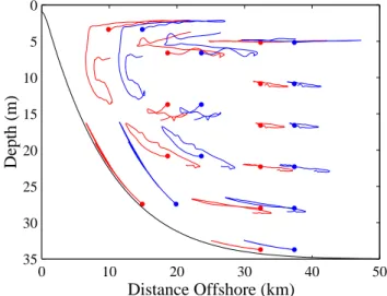
Fig. 5. Lagrangian parcel paths during one period beginning at
ti=9.25 T (red). The paths during a second period beginning at ti=10.25 T are shown in blue with a 5 km offset. The dots denote the initial locations of the parcels.
step (1ti). To determine the effect of the time step used to
solve Eq. (5), we also computed results using 1t=1ti/2,
which involves interpolation of the model velocities to this time. The results were quantitatively similar for both cases.
The updated positions obtained by solving Eq. (5) are saved hourly for each initial parcel position. Interpolation of all three components of velocity to the parcel positions after each iteration is bilinear. Lagrangian results from ad-ditional experiments using bicubic interpolation of the ve-locity fields to the parcel positions were quantitatively sim-ilar to those using bilinear interpolation. Although many of the model parcel paths exhibit considerable complexity, they are closely similar from one period to the next (Fig. 5). The only region in which significant discrepancy exists is near the coastal boundary from about 5–15 m depth. This region will be shown in Sect. 4 to produce complex and irregular parcel displacement patterns.
In addition to tracking individual water parcels, we uti-lize a second technique that gives Lagrangian trajectories for a continuous field of parcels. This approach involves the definition of three Lagrangian label fields that are advected by the model velocities. The Lagrangian labels, X(x, z, t ),
Y (x, y, z, t ), and Z(x, z, t ), satisfy the following equations:
DX Dt =0, DY Dt =0, DZ Dt =0, (6) where DtD=∂ ∂t+u ∂ ∂x+v ∂ ∂y+w ∂
∂z. The initial conditions are X(x, z, t =0) = x,
Y (x, y, z, t =0) = y,
−0.02 0 0.02 0 10 20 30 40 50 0 5 10 15 20 25 30 35
Eulerian
U (m s
−1)
−0.01 0 0.01 0 10 20 30 40 50 0 5 10 15 20 25 30 35W (10
−3m s
−1)
−0.05 0 0.05 0 10 20 30 40 50 0 5 10 15 20 25 30 35V (m s
−1)
−0.02 0 0.02 0 10 20 30 40 50 0 5 10 15 20 25 30 35Velocity
Stokes
Initial Distance (km) −0.05 0 0.05 0 10 20 30 40 50 0 5 10 15 20 25 30 35 Initial Distance (km) −0.02 0 0.02 0 10 20 30 40 50 0 5 10 15 20 25 30 35Tracking
Parcel
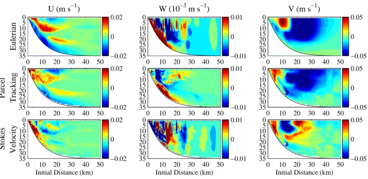
−0.05 0 0.05 0 10 20 30 40 50 0 5 10 15 20 25 30 35 −0.01 0 0.01 0 10 20 30 40 50 0 5 10 15 20 25 30 35 Initial Distance (km) −0.01 0 0.01 0 10 20 30 40 50 0 5 10 15 20 25 30 35Fig. 6. Mean Eulerian (Eq. 13) (top), Lagrangian (Eq. 14) (middle), and Stokes (Eq. 12) (bottom) velocities computed over one period
beginning at ti=9.25 T. u is across-shelf, w is vertical, and v is along-shelf.
With the two-dimensional approximation for the Eulerian flow we obtain
D Dt
∂Y
∂y=0. (8)
Thus, we can write
Y (x, y, z, t ) = y + Y0(x, z, t ), (9) and we can determine Y by solving for Y0, where
DY0
Dt +v=0, (10)
with
Y0(x, z, t =0) = 0. (11)
The labels X, Y and Z are calculated as fields on the model grid with the higher-order accurate advection scheme of Smolarkiewicz (1983) using three iterations of the correc-tive step. We note that the evolution of the Lagrangian label fields is completely determined by advection with the model-resolved velocity fields. Consequently, the behaviour of the labels will differ from that of passive tracer fields that are diffused by the effects of small-scale turbulence. This differ-ence is shown explicitly by analysis of results from related solutions in KC2003.
3 Dynamical analysis 3.1 Mean velocities
The one period means of the Eulerian, Lagrangian and Stokes velocities (Fig. 6) show a response to both upwelling and
downwelling forcing. The mean Stokes velocity is defined here as the difference between the mean Lagrangian and Eu-lerian velocities:
¯
uS(x(ti), z(ti)) = ¯uL(x(ti), z(ti))
− ¯uE(x(ti), z(ti)), (12) where ¯ uE(x(ti), z(ti)) = 1 T tf Z ti uE(x(ti), z(ti), t )dt, (13) ¯ uL(x(ti), z(ti)) = x(tf) − x(ti) T , ¯ wL(x(ti), z(ti)) = z(tf) − z(ti) T , ¯
vL(x(ti), z(ti), y(ti)) = y(tf)
T . (14)
and T = tf −ti.
The mean Eulerian across-shelf velocity u shows onshore flow of 2 cm s−1 in the bottom layer and offshore flow at
about 5–15 m depth from 0–20 km offshore. A classical steady upwelling response would exhibit offshore flow in the surface layer and onshore return flow in the bottom layer (as in Fig. 3 at t=9.25 T). The response here resembles such an upwelling circulation, but the location of the maximum off-shore velocity is shifted from the surface layer downward due to the downwelling phase of the circulation. There also exists a region of onshore flow in the top 5 m and a region of off-shore flow between 20–25 m depth from 10–20 km offoff-shore. The pattern of mean onshore surface u and offshore u below
arises because the surface layer during upwelling is thicker than that during downwelling from 10–20 km offshore. The dynamics of this response are described in Sect. 4.1.
The Lagrangian across-shelf velocity computed from the parcel tracking technique shows a similar pattern. The Stokes velocity quantifies the differences between the Eulerian and Lagrangian mean velocities. The most significant difference is located near the bottom from the coast to 8 km offshore. The mean Lagrangian u is offshore in this region, whereas the Eulerian u is onshore, leading to large positive Stokes drift values. Parcels that are initialized in this region have a net offshore displacement, despite the mean onshore Eulerian velocity, because they are advected vertically up the shelf and then offshore over a forcing period.
The mean Eulerian along-shelf velocity v shows a north-ward coastal upwelling jet of 5 cm s−1and a region of similar
magnitude southward velocities from 20–40 km offshore and extending to 20 m depth. This pattern results from a nar-row northward coastal jet during upwelling and a broader southward current during downwelling. The Lagrangian along-shelf velocity pattern is similar, although the north-ward coastal jet is distorted in x and z and located closer to the coast. The Stokes velocity reflects this difference, as well as the larger southward Eulerian v values offshore of 15 km. The Eulerian vertical velocity w is rather noisy, but shows upward velocities near the coast due to upwelling, and downward velocities just offshore due to downwelling. The Lagrangian vertical velocity shows a similar pattern from the coast to 12 km offshore, without the small-scale features seen in the Eulerian field. The vertical Stokes velocity reflects the consistently larger Eulerian w values and the patch of nega-tive Eulerian w from 12–20 km that is not found in the mean Lagrangian w.
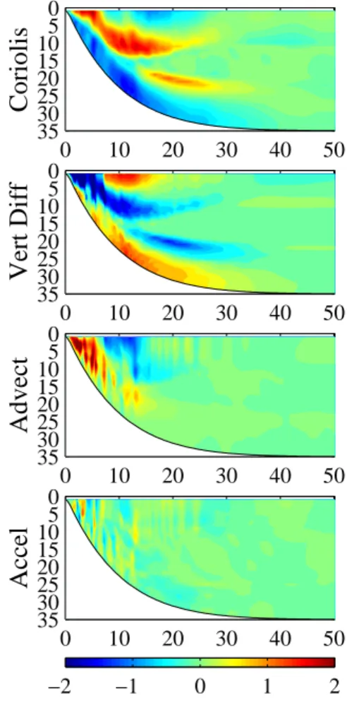
3.2 Nonlinear Advection
The dominant balance in the one period mean of the along-shelf momentum balance for a cycle beginning at ti=9.25 T
is between the Coriolis and vertical diffusion terms (Fig. 7). Within the first 12 km of the coast, the nonlinear advection term also plays an important role. The nonlinear term is also important in the explanation of dynamical differences be-tween the upwelling and downwelling responses (KC2003). We investigate these differences further by looking at mean fields computed over each half period with upwelling and downwelling forcing beginning at ti=9 T (Fig. 8). The
streamfunction ψ is defined as ψσ=uD, ψx= −ω. The
non-linear advection term may be written as u·∇v=uvx+wvz,
which corresponds to a spatial derivative of v in a direction tangent to the streamlines ψ =constant. The relative inten-sity of the across-shelf circulation can be estimated from the spacing of the streamlines. Thus, the magnitude of the term
u·∇v can be qualitatively assessed from the streamline
spac-ing and the gradient of v along streamlines. The stream-lines show very similar across-shelf circulation values dur-ing upwelldur-ing and downwelldur-ing, with opposite signs to in-dicate the reversed sense of circulation between upwelling
0 10 20 30 40 50 0 5 10 15 20 25 30 35
Coriolis
0 10 20 30 40 50 0 5 10 15 20 25 30 35Vert Diff
0 10 20 30 40 50 0 5 10 15 20 25 30 35Advect
−2 −1 0 1 2 0 10 20 30 40 50 0 5 10 15 20 25 30 35Accel
Fig. 7. Mean along-shelf momentum balance terms over one period
beginning at ti =9.25 T. The signs of the terms correspond to all terms on the left-hand side of the equation. The units for each term are 10−6m s−2.
and downwelling. The along-shelf velocity during upwelling shows a northward coastal jet from 0–15 km offshore and a region of southward velocities just offshore. During down-welling, however, the strongest along-shelf velocity values extend to 35 km offshore, with a region of much weaker ve-locity from 5–10 km offshore. This structure exhibits weaker across-shelf and vertical gradients in v, which lead to smaller magnitude values for the nonlinear term during downwelling. The nonlinear term during downwelling is only significantly different from zero in a few small bands of about 1 km width (Fig. 8, bottom right panel). During upwelling, the nonlinear term is large and positive from 2–6 km offshore, and large and negative from 10–20 km offshore. The structure of the nonlinear advection term during upwelling also closely re-sembles that of the mean field over a period (Fig. 7). There-fore, the nonlinear advection term makes a significant contri-bution to the along-shelf momentum balance during the up-welling phase of the forcing period, but a relatively small contribution during the downwelling phase.
−0.1 −0.05 0 0.05 0.1 0.15 0.2 0 5 10 15 20 25 30 35 40 45 50 0 5 10 15 20 25 30 35 −0.45 −0.1 Mean V (m s − 1 )
Upwelling Half Period
−0.2 −0.15 −0.1 −0.05 0 0.05 0.1 0 5 10 15 20 25 30 35 40 45 50 0 5 10 15 20 25 30 35
Downwelling Half Period
0.1 0.45 −3 −2 −1 0 1 2 3 0 5 10 15 20 25 30 35 40 45 50 0 5 10 15 20 25 30 35 Mean −0.1 −0.45 (uv) x + (wv) z (10 − 6 m s − 2 ) −3 −2 −1 0 1 2 3 0 5 10 15 20 25 30 35 40 45 50 0 5 10 15 20 25 30 35 0.1 0.45
Fig. 8. Mean of along-shelf velocity
(top) and the nonlinear advection term from the along-shelf momentum bal-ance (bottom) over the half period with upwelling forcing, t=9 T–9.5 T (left), and downwelling forcing, t=9.5 T–10 T (right). The streamlines are also plotted as black contours. 0 10 20 30 40 50 0 10 20 30
X
9.25T
0 10 20 30 40 50 0 10 20 309.5T
0 10 20 30 40 50 0 10 20 309.75T
0 10 20 30 40 50 0 10 20 3010T
0 10 20 30 40 50 0 10 20 3010.25T
0 10 20 30 40 50 0 10 20 30Z
0 10 20 30 40 50 0 10 20 30 0 10 20 30 40 50 0 10 20 30 0 10 20 30 40 50 0 10 20 30 0 10 20 30 40 50 0 10 20 30 0 10 20 30 40 50 0 10 20 30Y
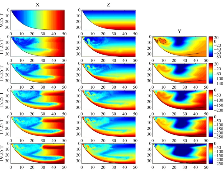
0 10 20 30 40 50 0 10 20 30 0 10 20 30 40 50 0 10 20 30 −40 −20 0 20 40 0 10 20 30 40 50 0 10 20 30Fig. 9. Contours of Lagrangian label fields every quarter period during one period beginning at ti=9.25 T. The Y label has units of km and
0 10 20 30 40 50 0 10 20 30
X
9.25 T
0 10 20 30 40 50 0 10 20 3011.25 T
0 10 20 30 40 50 0 10 20 3013.25 T
0 10 20 30 40 50 0 10 20 3015.25 T
0 10 20 30 40 50 0 10 20 3017.25 T
0 10 20 30 40 50 0 10 20 3019.25 T
0 10 20 30 40 50 0 10 20 30Z
0 10 20 30 40 50 0 10 20 30 0 10 20 30 40 50 0 10 20 30 0 10 20 30 40 50 0 10 20 30 0 10 20 30 40 50 0 10 20 30 0 10 20 30 40 50 0 10 20 30 −80 −60 −40 −20 0 20 0 10 20 30 40 50 0 10 20 30Y
−140 −100 −60 −20 20 0 10 20 30 40 50 0 10 20 30 −200 −150 −100 −50 0 0 10 20 30 40 50 0 10 20 30 −250 −200 −150 −100 −50 0 0 10 20 30 40 50 0 10 20 30 −250 −200 −150 −100 −50 0 0 10 20 30 40 50 0 10 20 30Fig. 10. Contours of Lagrangian label fields every two periods during a ten-period simulation beginning at ti=9.25 T. The Y label has units
of km and the black line marks the 0 contour for Y .
4 Lagrangian parcel paths 4.1 Lagrangian label field results
The time evolution of the Lagrangian label fields X, Y , and Z introduced in Sect. 2.3 provide an effective way to visualize the across-shelf, along-shelf, and vertical displacements of water parcels on the shelf. We show the evolution of these fields throughout a forcing period beginning at ti=9.25 T
by plotting their distributions at t =9.5 T, 9.75 T, 10 T, and 10.25 T (Fig. 9). At 9.5 T, the X label shows surface parcels have moved about 10 km offshore, while bottom parcels have moved about 5 km onshore as the response in the bottom layer is slower than that in the surface. Parcels near the sur-face move onshore close to their initial locations at 9.75 T while most of the bottom layer parcels have not moved sig-nificantly since 9.5 T. At 10 T, parcels in the surface layer are displaced 10 km onshore and parcels in the bottom layer have retreated offshore toward their initial across-shelf loca-tion. After a full period, surface parcels are advected offshore again near their initial positions. The final distribution of X
shows a feature of offshore displacement at 20 m depth from 15–35 km offshore and several interlacing features inshore of 20 km. The former is due to the thicker bottom bound-ary layer that is present during downwelling than during up-welling, ascribed by Lentz and Trowbridge (1991) to the upslope (upwelling) or downslope (downwelling) transport of buoyancy along the bottom. During upwelling, the ups-lope transport of denser water under lighter water enhances the stratification and inhibits growth of the bottom boundary layer. In contrast, the downslope transport of lighter water under heavier water during downwelling tends to enhance mixing and thus, leads to growth of the bottom boundary layer. During downwelling, parcels are displaced offshore in a 10–15 m thick bottom layer. However, during upwelling, the bottom layer is only 5–10 m thick, therefore parcels in this thinner bottom boundary layer are displaced onshore and parcels just above it are displaced offshore relative to their initial positions after one period.
A similar physical argument applied to the surface layer supports the pattern of u in Fig. 3 and the feature of offshore displacement of X just below the surface from 10–20 km
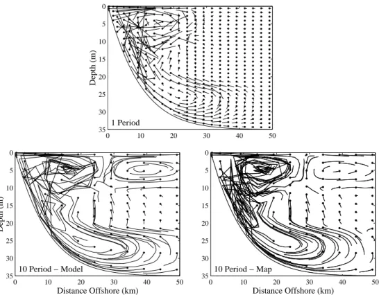
0 10 20 30 40 50 0 5 10 15 20 25 30 35 1 Period Depth (m) 0 10 20 30 40 50 0 5 10 15 20 25 30 35 10 Period − Map Distance Offshore (km) 10 Period − Map 0 10 20 30 40 50 0 5 10 15 20 25 30 35 10 Period − Model Depth (m) Distance Offshore (km)
Fig. 11. Lagrangian parcel displacements over one period (top) and over ten periods computed from the model (bottom left) and mapping
technique (bottom right) for a simulation beginning at ti=9.25 T. The dots denote the initial locations of the parcels.
offshore in Fig. 9. In this case, upwelling transports heav-ier water to the surface, enhancing mixing and producing a thicker surface boundary layer. Downwelling transports lighter water onshore which inhibits mixing and leads to the net onshore displacement of green X labels at the surface from 10–20 km offshore (Fig. 9).
The evolution of Z in Fig. 9 shows complicated structures that develop during both upwelling and downwelling. At 9.75 T, a thin layer of parcels initialized at mid-depth has been advected upward toward the coast due to upwelling. After downwelling begins, the 10 T distribution shows part of this thin layer of Z parcels remains trapped at the coast because the downwelling response is weak inshore of about 5 km.
The Y label field shows along-shelf advection of up to 40 km to the north (red) and south (blue). The re-gion of northward parcel advection in the coastal up-welling jet moves onshore and increases in magnitude from 9.5 T–9.75 T. After a quarter-period of downwelling forc-ing (10 T), however, the region of northward displacements has decreased significantly in size and magnitude and south-ward displacements are found offshore near the surface. The quarter-period of upwelling forcing from 10 T–10.25 T does not significantly increase the northward displacements in this region, as might be expected, but only moves the jet up the shelf. Southward displacements exist over a region of rela-tively large offshore extent from x=15−35 km. The Y
re-sponse reflects the lag of along-shelf parcel advection after the along-shelf wind changes direction discussed in Sect. 2.2 (Fig. 4).
Net displacements of water parcels over many forcing pe-riods, or several upwelling and downwelling events, can also be described by the evolution of the Lagrangian label fields
X, Y , and Z (Fig. 10). After two periods, the distributions of X, Y , and Z look very similar to those after one period in Fig. 9. The feature at 20 m depth in X that was described due to the difference in bottom boundary layer thickness during upwelling and downwelling becomes more pronounced with each additional forcing period. It also appears in the Z field after 4 periods (t=13.25 T). The region of trapped parcels near the coast, as shown by Z, grows in time and the initial position of the trapped parcels becomes deeper (colours near the coast change from yellow to red). Net onshore displace-ment of X occurs at about 5–10 m depth offshore of 30 km. Between these features at mid-depth offshore of 30 km, there is very little horizontal or vertical motion. Onshore of 30 km, however, parcel displacements are complicated and there is significant across-shelf and vertical motion.
The region of southward along-shelf displacements (Y ) increases in both size and magnitude as the parcels are ad-vected farther south over a broader region of the shelf with each forcing period. In contrast, the inshore region of north-ward displacements shrinks in size and decreases in mag-nitude. This result is robust for simulations beginning at
any point in the forcing period (8.5 T, 8.75 T, 9 T, or 9.25 T). Thus, after several periods, parcels at almost all depths from 0–50 km will be displaced south of their initial position, in-dependent of the initial forcing phase. Evidently, the rea-son for this is that parcels do not remain in the region of the northward upwelling jet, where they would be advected farther northward, but instead move offshore into the broad region of southward velocities (see the mean Lagrangian u and v in Fig. 6).
4.2 Fluid parcel tracking results
We also investigate parcel displacements over a forcing pe-riod using the parcel tracking method introduced in Sect. 2.3 for a simulation with ti=9.25 T and parcels initialized at
ev-ery grid point on the model domain (Fig. 11, top panel). Some regions show net displacements over a period that agree well with the label fields (Fig. 9), while other regions are more complicated. Parcels in the bottom 5 m of the shelf move onshore with displacement values that increase as the initial position of the parcel nears the coast. Offshore dis-placement, due to the thicker bottom boundary layer during downwelling, of parcels initially between 15–45 km is ap-parent above the bottom layer. At mid-depth and offshore of 20 km, parcels are shown to move slightly downward over a forcing period. In the surface layer offshore of 30 km, a cell structure is seen with parcels moving offshore above 5 m and onshore from 5–10 m depth. The parcel motion near the coast is complicated with parcel displacements that cross one another and vary in length and direction. It is unclear whether all of this complexity is due to the true motion re-solved by the model, or if small errors in the parcel tracking calculation make a contribution in this region. The results of the Lagrangian label analysis also show this region produces significant parcel displacements and complex paths over one period (Fig. 9) or ten periods (Fig. 10). Thus, we are confi-dent in the general conclusion that complex parcel paths exist in this region, although care must be taken in interpreting in-dividual parcel trajectories.
4.2.1 Parcel displacement maps
Due to the near periodicity of the response, we can use a mapping technique to calculate the parcel displacements over many periods without actually tracking them in the model simulation. The map is created from the one-period model parcel displacements (Fig. 11, top panel). Using a bilinear interpolation, the net displacement of each parcel in x and z may then be iterated forward for as many periods as desired. This mapping technique can thus, provide a description of parcel displacements over many periods at very little compu-tational cost. The map is an extremely useful tool that helps determine the qualitative Lagrangian behaviour and gives a clear picture of parcel displacement trends. Implementing the one-period displacement map technique, we effectively approximate the Eulerian flow as periodic. The qualitative accuracy of this approximation is supported by Figs. 2 and 5,
as well as the bottom panels of Fig. 11, which show that the iterated map reproduces the features of the ten-period model parcel displacements reasonably well. The model displace-ments tend to be larger than those produced from the iterated map in some locations. Again, the complicated region near the coast exhibits the largest quantitative differences because the model displacements are not entirely reproducible from one period to the next in this area (Fig. 5), hence the iterated-map trajectories diverge slowly from the model trajectories.
We performed simulations with varying horizontal and vertical resolution to determine the sensitivity of the Eulerian and Lagrangian results on model resolution. For ti=9.25 T,
we computed model Eulerian fields, Lagrangian labels, and parcel trajectories over one period with 1x=125 m and 45 σ levels to compare with the basic case resolution of
1x=250 m and 30 σ levels. Parcels were located at each grid point in both simulations. The results of the mean Eulerian fields, Lagrangian label evolution, and 10 period parcel maps were quantitatively similar in both cases.
The Lagrangian results depend on the simulation start time because this determines the phase of the model Eule-rian velocity field. We investigate the dependence of the 100 period Lagrangian maps on the simulation start time by plotting selected parcel positions after each period for
ti=8.5 T, ti=8.75 T, ti=9 T, and ti=9.25 T (Fig. 12). The
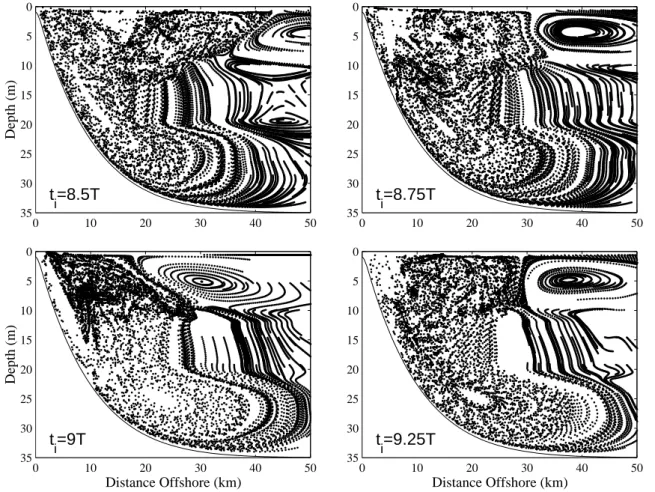
same structures are seen in all of these maps, however they are located in different across-shelf and, in some cases, verti-cal, locations. The maps show regions with well-defined pe-riodic motion and regions with a more complex response to periodic forcing. A rotating cell feature (offshore of 30 km at ti=8.75 T) and the slow downward motion at mid-depth
are apparent. The previously described feature with offshore displacement from 20–25 m depth and onshore displacement below is seen. Inshore of 30 km, the parcel displacements do not exhibit any regular patterns. Parcels that upwell to the near surface close to the coast are typically displaced off-shore within the complex region. A clear boundary between this region and the offshore surface cell is apparent (e.g. at 30 km offshore at ti=8.75 T) in which parcels above 10 m
depth move upward and offshore into the cell.
The evolution of parcels in the cell structure and other parcels on the shelf is explained by the upwelling and down-welling dynamics over a forcing period and can be deter-mined by studying the sequential maps (Fig. 12). The surface cell feature is displaced offshore of 30 km for ti=8.5 T and
onshore for ti=9 T. For ti=9.25 T, the location is similar to
that for ti=8.75 T. The orientation of the boundary between
this structure and the complex region inshore also varies. Parcels offshore of 30 km in the top 5 m are displaced on-shore about 20 km during the half cycle t =8.5 T–9 T, and parcels from 5–10 m are displaced about 10 km onshore. From 10–20 m depth, parcels are displaced 5 km offshore and below this, in the bottom boundary layer region, parcels are displaced about 10 km offshore. Near the coast the across-shelf motion is not as clear and vertical motion is sig-nificant.
0 10 20 30 40 50 0 5 10 15 20 25 30 35
t
i=8.5T
Depth (m) 0 10 20 30 40 50 0 5 10 15 20 25 30 35t
i=8.75T
0 10 20 30 40 50 0 5 10 15 20 25 30 35t
i=9T
Distance Offshore (km) Depth (m) 0 10 20 30 40 50 0 5 10 15 20 25 30 35t
i=9.25T
Distance Offshore (km)Fig. 12. Lagrangian parcel positions after each period predicted by mapping technique over 100 periods for simulations beginning at ti=8.5 T,
ti=8.75 T, ti=9 T, and ti=9.25 T.
To quantify the motion of the cell feature over a forcing period, consider the trajectory of a single parcel initialized at ti=8.5 T at x=48.875 km, z= − 4.0783 m (the
approxi-mate center of the offshore surface cell) (Fig. 13a). Subject to downwelling forcing initially, the parcel moves 9 km onshore in the first quarter-period and 11 km onshore in the second quarter-period. After upwelling winds begin at t =9 T, the parcel moves offshore 8 km during the third quarter-period and another 12 km in the final quarter-period. Total vertical displacement over a period is only about 0.2 m. The final position of the parcel is almost exactly the same as its initial position. Thus, the net across-shelf displacement of a parcel near the cell center over a period is very small even though it is advected 20 km across the shelf during each phase of the forcing period. Figure 13a shows movement of the cell center and clearly illustrates why the maps constructed at different phases of the forcing cycle have different structures.
Consider a second parcel initialized at ti=8.5 T at x=37.375 km, z= − 4.0448 m (Fig. 13b). The parcel travels about 20 km onshore during downwelling and 20 km offshore during upwelling. The position after one period, at t =9.5 T, is about 1 m above the initial position and the position after two periods at t =10.5 T is 1 m above that at t =9.5 T. The parcel has a net offshore displacement of 1 km during each
of these periods. In contrast, the net displacement of the par-cel is 1 km onshore over the period from t =9 T–10 T. Thus, the direction of displacement across the shelf differs for the upwelling half-period (onshore displacement) and the down-welling half-period (offshore displacement) for parcels in the region just onshore of the cell feature, and the net displace-ment over a full-period depends on the phase of the forcing at initialization due to the net vertical motion and the vertical shear of the time-dependent Eulerian flow.
4.2.2 Lyapunov exponents
Lyapunov exponents quantify exponential rates of diver-gence or converdiver-gence of the trajectories of initially neigh-boring particles in a flow field. Thus, they provide a mea-sure of the chaos present in a system. The Lagrangian results presented in Sects. 4.1 and 4.2 suggest that the parcel trajec-tories in the complicated region near the coast are chaotic. We examine this possibility and quantify the degree of chaos present in the wind-forced flows studied here by calculat-ing the largest Lyapunov exponent of the parcel displacement maps.
We estimate the largest Lyapunov exponent λ for the two-dimensional periodic map (see e.g. Benettin et al., 1976; Lichtenberg and Lieberman, 1983) from the truncated
approximation with finite M as: λ = 1 M1t M X i=1 ln Li L0i−1, (15)
where Li=(1xi2+1z2i)1/2 is the distance after the ith
cy-cle between two parcels initially separated by 1x0at t =t0
and Li0=(1xi02+1zi02)1/2 where 1xi0, 1z0i are rescaled val-ues of the estimated separations 1xi, 1zi given, if Li>1x0,
by 1xi0=1xi Li 1x0, 1z 0 i= 1zi Li 1x0so that L 0 i=L0=1x0. The
calculation of Liis made after each iterated period for every
parcel initialized on the map grid at (x0, z0) and a
neigh-boring parcel initialized at (x0+1x0, z0). If Li>1x0, the
distance between parcels is rescaled such that the neigh-boring parcel is re-positioned from (xi+1xi, zi+1zi) to (xi+1xi0, zi+1z0i)to keep the calculation near linear as
par-cel separations increase. If Li ≤1x0, then we do not rescale
so that 1x0i=1xi, 1z0i=1zi, and L0i=Li. The map is then used to determine the positions of the grid of neighboring parcels after any necessary rescaling has been done. The cal-culation was tested by varying the initial separation distance
1x0by 1x0=1xgrid/n(where 1xgrid=250 m, the grid
res-olution of the model and the map), and n=1, 2, 4, 8, 16, 32, 64. We also performed tests with an initial separation in the vertical direction of 1z0such that the grid of
neigh-boring parcels was initialized at (x0, z0+1z0). The largest
Lyapunov exponent was estimated for both positive and neg-ative values of 1x0, 1z0 and the results were qualitatively
similar in all cases. As 1x0decreased, the small differences
between results for the positive and negative initial separa-tions also decreased.
Estimates for the largest Lyapunov exponent λ are cal-culated for M=100 forcing periods with 1x0=1xgrid/64
(Fig. 14). Plots of λ for selected parcels versus t−1=(i1t )−1
indicate that the choice of M = 100 gives reasonable, but not fully convergent, approximations for the values of λ. Values of λ are largest in the region with complex parcel displace-ments near the coast and in the bottom 10 m. In these loca-tions, the magnitudes of λ are approximately 6–8. Offshore of 30–40 km from the surface to 25 m depth, values decrease to near zero, indicating regular behaviour. Negative values in this region, which presumably would asymptote to zero, are generally small, e.g. the minimum value is −0.75. The boundary at 30 km between large, positive λ in the top 10 m and small λ offshore divides the region of irregular and com-plicated parcel paths from the regular motion found in the surface cell feature. The location of this boundary is a robust result for any sufficiently large number of periods M. The small λ values below the surface cell feature correspond to the mid-depth region of slow downward parcel motion.
5 Summary
The Eulerian and Lagrangian dynamics of a wind-forced continental shelf have been studied using a numerical model forced by periodic winds. The mean Eulerian velocities show
25 30 35 40 45 50 4 4.1 4.2 4.3 4.4
Depth (m)
(a) 15 20 25 30 35 40 1 2 3 4 5Distance Offshore (km)
Depth (m)
(b)Fig. 13. Lagrangian parcel positions (a) during one period for
a parcel initialized at ti=8.5 T at x=48.875 km, z= − 4.0783 m and (b) during two periods for a parcel initialized at ti=8.5 T at x=37.375 km, z= − 4.0448 m. The red dot is the initial position, the blue dot is the position at t=8.75 T, green dot at t=9 T, and black dot at t=9.25 T. The colours repeat for the second period positions in (b) with smaller dots. The final parcel position is given by the red ×. −1 0 1 2 3 4 5 6 0 10 20 30 40 50 0 5 10 15 20 25 30 35 Depth (m) Distance Offshore (km)
Fig. 14. Largest Lyapunov exponent λ computed from the
map-ping technique after 100 forcing periods beginning at ti=9.25 T. The black line denotes the 0 contour.
features from both the upwelling and downwelling phases of the period. Near the surface, there is offshore flow from the coast to 30 km due to upwelling and onshore flow just above due to downwelling. In the bottom layer, onshore flow due
to upwelling is in the bottom 5 m, and just above is a region of offshore flow due to downwelling, a result of the thicker bottom boundary layer during downwelling. In the along-shelf momentum balance, nonlinear advection of momentum is stronger during the upwelling phase. This result is linked to the weaker across-shelf and vertical gradients in the along-shelf velocity during downwelling.
Lagrangian motion was analyzed using Lagrangian label fields and a parcel tracking technique. The labels show sig-nificant across-shelf, along-shelf, and vertical advection over a period. After several forcing periods, the bottom layer re-sponse becomes much more pronounced while the surface layer response weakens. Near the coast, a region of large
x and z displacements shows complex patterns in the label fields with variability in parcel trajectories from one period to the next. Net southward displacement increases and net northward displacement decreases in time, leading to the re-sult that all the parcels on the shelf are displaced to the south after many periods. Similar information can be obtained by tracking individual parcels in the traditional manner.
Results have also been obtained by iterating the one-period displacement map for many periods. The map is useful in providing a qualitative assessment of the Lagrangian motion of fluid parcels over many periods. The perspective on parcel motion over one period gained from the analysis of these iter-ated maps is valuable as well. By following the progression of maps initialized at different forcing phases, the displace-ment of parcels in different regions of the shelf can be iden-tified. The rotating surface cell offshore of 30 km appears especially clearly in this analysis. The map also makes possi-ble the calculation of approximate values for the largest Lya-punov exponent, which quantifies to some extent the chaos present in the region of complicated parcel paths near the coast.
Except near the center of the offshore surface cell, parcels generally do not return to their initial location after a period, hence a Stokes drift exists and is maximum in the complex region near the coast. Parcel displacement depends on the initial location and the initial forcing phase. Asymmetries between the upwelling and downwelling responses lead to significant net across-shelf displacements in the surface and bottom layers. The complex motion of Lagrangian parcels in three dimensions leads to interesting results that are not obvi-ously suggested by the Eulerian fields. One clear example is the robust southward along-shelf displacement of all parcels after several periods.
Acknowledgements. This research was supported by the Office of
Naval Research (ONR) Coastal Dynamics Program through grant N00 014–02–1–0100. Additional support was provided by the National Science Foundation through NSF grant OCE–9907854 and for R.M.S. by the ONR Ocean Modeling and Prediction Program through ONR grant N00014–98–1–0813.
Edited by: S. Wiggins Reviewed by: one referee
References
Austin, J. A. and Lentz, S. J.: The relationship between synoptic weather systems and meteorological forcing on the North Car-olina inner shelf, J. Geophys. Res., 104, 18 159–18 185, 1999. Benettin, G., Galgani, L., and Strelcyn, J. M.: Kolmogorov entropy
and numerical experiments, Phys. Rev. A, 14, 2338–2345, 1976. Blumberg, A. F. and Mellor, G. L.: A Description of a Dimensional Coastal Ocean Circulation Model, Three-Dimensional Coastal Ocean Models, Coastal and Estuarine Sci-ence Series, Vol. 4, N. Heaps Ed., AGU, 1–16, 1987.
Coulliette, C. and Wiggins, S.: Intergyre transport in a wind-driven, quasigeostrophic double gyre: An application of lobe dynamics, Nonl. Pr. Geo., 8, 69–94, 2001.
Galperin, B., Kantha, L. H., Hassid, S., and Rosati, A.: A quasi-equilibrium turbulent energy model for geophysical flows, J. At-mos. Sci., 45, 55–62, 1988.
Haller, G.: Lagrangian coherent structures from approximate veloc-ity data, Physics of Fluids, 14, 1851–1861, 2002.
Ide, K., Small, D., and Wiggins, S.: Distinguished hyperbolic tra-jectories in time-dependent fluid flows: analytical and computa-tional approach for velocity fields defined as data sets, Nonl. Pr. Geo., 9, 237–263, 2002.
Kirwan, A. D., Toner, M., and Kantha, L.: Predictability, uncer-tainty, and hyperbolicity in the ocean, Int. J. Engin. Sci., 41, 249–258, 2003.
Kuebel Cervantes, B. T., Allen, J. S., and Samelson, R. M.: A Mod-eling Study of Eulerian and Lagrangian Aspects of Shelf Circu-lation off Duck, North Carolina, J. Phys. Ocea., 33, 2070–2092, 2003.
Lentz, S. J. and Trowbridge, J. H.: The bottom boundary layer over the northern California shelf, J. Phys. Ocea., 21, 1186–1201, 1991.
Lichtenberg, A. J. and Lieberman, M. A.: Regular and Stochastic Motion, Springer-Verlag, New York, NY, 499, 1983.
Loder, J. W., Shen, Y., and Ridderinkhof, H.: Characterization of Three-Dimensional Lagrangian Circulation Associated with Tidal Rectification over a Submarine Bank, J. Phys. Ocea., 27, 1729–1742, 1997.
Mellor, G. L. and Yamada, T: Development of a Turbulence Clo-sure Model for Geophysical Fluid Problems, Rev. Geophys. and Space Phys., 20, 851–875, 1982.
Miller, P. D., Jones, C. K. R. T., Rogerson, A. M., and Pratt, L. J.: Quantifying transport in numerically generated velocity fields, Physica D, 110, 105–122, 1997.
Poje, A. C. and Haller, G.: Geometry of Cross-Stream Mixing in a Double-Gyre Ocean Model, J. Phys. Ocea., 29, 1649–1665, 1999.
Poje, A. C., Toner, M., Kirwan, A. D., and Jones, C. K. R. T.: Drifter Launch Strategies Based on Lagrangian Templates, J. Phys. Ocea., 32, 1855–1869, 2002.
Ridderinkhof, H. and Loder, J. W.: Lagrangian Characterization of Circulation over Submarine Banks with Application to the Outer Gulf of Maine, J. Phys. Ocea., 24, 1184–1200, 1994.
Rom-Kedar, V., Leonard, A., and Wiggins, S.: An analytical study of transport, mixing and chaos in an unsteady vortical flow, J. Fluid Mech., 214, 347–394, 1990.
Smolarkiewicz, P. K.: A Simple Positive Definite Advection Scheme with Small Implicit Diffusion, Mon. Wea. Rev., 111, 479–486, 1983.
Weiss, J. B. and Knobloch, E.: Mass transport and mixing by mod-ulated traveling waves, Phys. Rev. A, 40, 2579–2589, 1989.