Drivers of photovoltaics cost evolution

(1)

Drivers of photovoltaics cost evolution

by

Goksin Kavlak

B.S. Industrial Engineering, Bogazici University, 2010 M.E.Sc. Environmental Science, Yale University, 2012 Submitted to the Institute for Data, Systems, and Society

in partial fulfillment of the requirements for the degree of DOCTOR OF PHILOSOPHY

at the

MASSACHUSETTS INSTITUTE OF TECHNOLOGY February 2018

c

Author . . . . Institute for Data, Systems, and Society

September 30, 2017 Certified by . . . .

Jessika E. Trancik Associate Professor of Data, Systems, and Society Thesis Supervisor and Doctoral Committee Chair Certified by . . . . Robert L. Jaffe Otto (1939) and Jane Morningstar Professor of Science Professor of Physics Doctoral Committee Member Certified by . . . . Joel P. Clark Professor of Materials Science and Engineering Doctoral Committee Member Accepted by . . . .

Stephen C. Graves Professor of Mechanical Engineering and Engineering Systems Abraham J. Siegel Professor of Management Science IDSS Graduate Officer

(2)

(3)

Drivers of photovoltaics cost evolution by

Goksin Kavlak

Submitted to the Institute for Data, Systems, and Society on September 30, 2017, in partial fulfillment of the

requirements for the degree of DOCTOR OF PHILOSOPHY

Abstract

Photovoltaics (PV) have experienced notable development over the last forty years. PV module costs have declined 20% on average with every doubling of cumulative capacity, while global PV installations have increased at an average rate of 30% per year. However, costs must fall even further if PV is to achieve cost-competitiveness at high penetration levels and in a wide range of locations. Understanding the mechanisms that underlie the past cost evolution of PV can help sustain its pace of improvement in the future.

This thesis explores the drivers of and constraints to cost reduction and large-scale deployment of PV. By developing novel conceptual and mathematical models, we address the following questions: (1) What caused PV’s cost to fall with time? (2) How may materials constraints influence PV cost and deployment? These questions are addressed in the analyses presented in Chapters 2-4.

Chapter 2 assesses the causes of cost reduction observed in PV modules since 1980. We develop a new model that identifies the causes of improvement at the engineering level and links these to higher-level mechanisms such as economies of scale. The methodology advanced can be used to evaluate the causes of improvements in any technology. By developing a model of PV modules, we find that in the early stages of the technology (1980-2001), improvements in the material usage and module conversion efficiency played an important role in reducing module cost. These improvements were mainly driven by research and development (R&D) efforts. As the PV technology matured (2001-2012), economies of scale from larger manufacturing plants resulted in significant gains. Both market-expansion policies and public R&D stimulated cost reduction, with the former contributing the majority of the cost decline from 1980 to 2012.

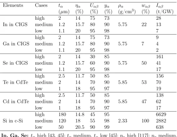
Chapter 3 turns to assessing the materials constraints to PV cost reduction. We ask how fast metals production should be scaled up to match the increasing demand by the PV sector, if installations grow to meet a significant portion of energy demand. Unlike previous studies, which primarily used inherently uncertain factors such as reserves to estimate limits to technology scalability, we use past growth rates of a large set of metals as a benchmark for future growth rates. This analysis shows that thin-film PV technologies such as CIGS and CdTe that employ rare metals would require unprecedented growth rates in metals production even for the most conservative PV growth scenarios. On the other hand, crystalline silicon PV can provide 100% of global electricity without silicon exceeding the historical growth rates observed by all metals in the periodic table.

Chapter 4 assesses the risks that material inputs bring to technologies today. This study develops cost-riskiness metrics based on the price behavior of metals along two dimensions: average price and price volatility. We first compare a large set of metals using these

(4)

cost-riskiness metrics. We observe that metals obtained as byproducts have higher risk than major metals. We then apply these metrics to different PV technologies by treating them as a portfolio of metals. We find that designs such as CIGS and CdTe, which use byproduct metals with high average prices and price volatilities, show signals of cost-riskiness. The approach advanced here can serve as an assessment of the cost-riskiness of technologies introduced by their materials inputs.

Jessika E. Trancik

Associate Professor of Data, Systems, and Society Thesis Supervisor and Doctoral Committee Chair Robert L. Jaffe

Otto (1939) and Jane Morningstar Professor of Science, Professor of Physics Doctoral Committee Member

Joel P. Clark

Professor of Materials Science and Engineering Doctoral Committee Member

(5)

Acknowledgments

This thesis would not have been completed without the support and encouragement of my mentors, colleagues, friends and family.

First and foremost I thank my advisor, Jessika Trancik. I am grateful to you for being my mentor and helping me grow as a researcher over the last five years. With your high standards and motivation, you are a role model that I look up to. I also thank my committee member, Robert Jaffe, for enlightening discussions and crucial feedback since I came to MIT. I thank my committee member Joel Clark for his helpful questions and support. I also thank James McNerney, a co-author on all of the three papers that form this thesis –this thesis would not be the same without his contribution. I also thank U.S. Department of Energy and MIT Energy Initiative for supporting this research.

I am grateful to have been part of the Institute for Data, Systems, and Society and

Engineering Systems Division communities. I thank Joe Sussman, Chris Magee, Lisa

d’Ambrosio, Oli de Weck, and Richard Larson for introducing me to engineering systems and guiding me in my academic training. I thank Fran Marrone, Erica Bates, Keeley Rafter, and especially Beth Milnes for their support in making this process easier.

I also thank the researchers and mentors in my academic journey before MIT. I have been fortunate to have had Thomas Graedel as a mentor while at Yale and to have benefited from his wisdom as he helped me transform from an undergraduate intern to a master’s student and a researcher. I thank Rob Bailis, Matthew Eckelman, Barbara Reck, Ermelinda Harper, and Chad Oliver as I learned immensely from them while working with them during my studies at Yale. I also thank my professors at my undergraduate institution, Bogazici University, especially Yaman Barlas, Gurkan Kumbaroglu, Aybek Korugan, and Kadri Ozcaldiran for supporting my transition to graduate studies.

I also want to extend my gratitude to my excellent colleagues and friends. I thank the current and former members and affiliates of the Trancik Lab for sharing their knowledge with me: Thank you to Morgan Edwards, Mandira Roy, Zach Needell, Joshua Mueller, Wei Wei, Marco Miotti, Magdalena Klemun, Goncalo Pereira, Hamed Ghoddusi, Michael Chang, Joel Jean, Patrick Brown. I also thank my friends who have supported me throughout my journey. Special thanks to Yin Jin Lee, Lita Das, Abby Horn, Adam Taylor, Maite Pena Alcaraz, Noel Silva Montero, Ioanna Karkatsouli, Ioanna Fampiou, Georgios Angelis, Giorgos

(6)

Faldamis, Iraz Topaloglu, Beyza Bulutoglu, Gal Zilberberg, Cristina Popa, and Kathryn Luly.

Finally, I would like to thank my parents Birsen and Ismail Kavlak and my brother Yetkin Kavlak for always being there for me, even though I am an ocean and a continent away. I dedicate this thesis to my parents.

(7)

List of Figures

2-1 Module costs and prices since 1975 . . . 23

2-2 Cost components for wafer, cell and module levels . . . 26

2-3 Contribution of the low-level mechanisms to module cost decline . . . 33

2-4 Contribution of the high-level mechanisms to module cost decline . . . 36

2-5 Contribution of market expansion policies to module cost reduction . . . 37

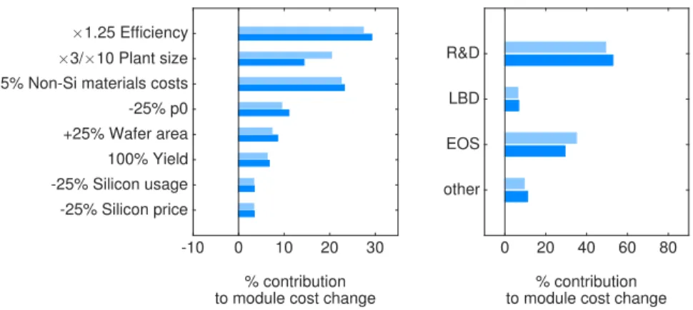
2-6 Module cost reductions from one-at-a-time changes to low-level variables . . . 40

2-7 Module cost reductions by changing several low-level variables simultaneously 41 3-1 Annual production of metals over time, 1972-2012 . . . 50

3-2 Historical growth rates for PV metals . . . 53

3-3 Histogram of the historical annual growth rates for 32 metals . . . 54

3-4 Required growth rates for PV metals production . . . 58

4-1 Average price versus average production for metals, 1973-2012 . . . 69

4-2 Average price and price volatility for different metal groups . . . 71

4-3 Metals price volatility for 1973-2012 . . . 72

4-4 Weighted price versus weighted price volatility for PV technologies . . . 75

A-1 Sensitivity analysis for silicon usage, 𝑣 . . . 80

A-2 Sensitivity analysis for silicon price, 𝑝𝑠 . . . 81

A-3 Sensitivity analysis for module efficiency, 𝜂 . . . 81

A-4 Sensitivity analysis for yield, 𝑦 . . . 82

A-5 Sensitivity analysis for wafer area, 𝐴 . . . 82

A-6 Sensitivity analysis for plant size, 𝐾 . . . 82

A-7 Sensitivity analysis for share of materials costs, 𝜃 . . . 83

(10)

A-9 Sensitivity analysis for scaling factor, 𝑏 . . . 83

A-10 Sensitivity analysis where all variables are varied . . . 84

A-11 Contribution of low-level mechanisms when silicon price in 1980 is varied . . . 84

A-12 Contribution of high-level mechanisms with alternate assignments . . . 86

A-13 Contribution of high-level mechanisms when they are reassigned one at a time 86 A-14 Highest and lowest contribution of R&D . . . 87

A-15 Highest and lowest contribution of learning-by-doing . . . 88

A-16 Highest and lowest contribution of economies of scale . . . 88

A-17 Contribution of high-level mechanisms by reassigning multiple variables at once 89 B-1 Historical production of MG-Si . . . 93

B-2 Required growth rates for MG-Si . . . 94

B-3 Year-to-year growth rates in metals production . . . 94

(11)

List of Tables

2.1 Data used to calculate module cost components. . . 27

2.2 Cost components in 1980, 2001 and 2012 . . . 30

2.3 Contribution of low-level mechanisms to module cost decline . . . 34

3.1 Cumulative Installed PV Capacity Projections for 2030 . . . 48

3.2 Parameters for Material Intensity . . . 49

4.1 Categorizing metals: Major metals, byproducts and others . . . 66

4.2 Average price and price volatility for metals in PV technologies . . . 74

A.1 Assignment of low-level mechanisms to high-level mechanisms . . . 85

A.2 Alternate assignments for the lowest and highest possible contributions of R&D 87 A.3 Alternate assignments for the lowest and highest possible contributions of learning-by-doing . . . 87

A.4 Alternate assignments for the lowest and highest possible contributions of economies of scale . . . 88

(12)

(13)

Chapter 1

Introduction

1.1 Research motivation

Photovoltaics (PV) may be an attractive energy technology for mitigating climate change. Solar energy is the largest energy resource on Earth [1]. Using current PV technology in less than 1% of the land area of the United States for a year, one could meet the yearly energy consumption of the nation [2]. Despite some variability in its temporal and geographical availability, solar energy is well-distributed across the world, unlike fossil fuels and hydropower [3]. PV technologies have low emissions from operation, while emissions during manufacturing and decommissioning solar panels have the potential to go to zero as these processes are increasingly powered by low-carbon sources [4].

Besides the characteristics that make PV a good candidate for climate change mitigation, PV is an extraordinary energy technology from a technological change perspective. The costs of renewable energy technologies have fallen dramatically over the last 40 years [5], and PV in particular was one of the most rapid among electricity technologies due to ongoing research, production and installation experience, and scale economies [6, 7]. As of 2015, silicon-based PV modules were roughly 100 times cheaper than they were 40 years ago [6]. Global PV deployment has also been growing rapidly, at over 30% per year in this period [8, 9].

Continued PV deployment could reduce greenhouse gas emissions [4] and other pollutants from energy systems [10]. For PV deployment to experience continued growth in the future, however, particularly when considering the additional costs of addressing solar intermittency [11], further cost reductions are likely needed [12]. For this reason, it is important to identify what drove PV’s past cost evolution to gain insight into maintaining the pace of improvement

(14)

in the future. In the process one may shed light on the drivers of technological progress in general.

Despite the rapid past decline in renewable energy technology costs, there may be constraints that could slow down or reverse these trends in the future. A relevant constraint for PV is materials [13, 14], which constitute a significant share of PV costs [15, 16, 17]. Increasing adoption of PV technologies at rates that would be relevant for climate change mitigation would require unprecedented growth in metals production [18, 19, 20]. Some current PV technologies use rare metals, e.g. tellurium and indium, which are obtained as byproducts of major metals such as copper and zinc [21, 22, 23]. Being byproducts, their price and production are dictated by the economics of the major metals that host them, giving rise to concerns about whether supply can meet demand increases [24, 25, 26, 27] with prices that remain stable enough for cost-effective PV production [28]. Assessing such materials constraints is critical for understanding the scalability of technologies, and sustaining high rates of deployment and cost improvement.

1.2 Background

Improvement trends in photovoltaics (PV) and other technologies have been studied by several research communities. One common approach, which we call ‘correlational analysis’, focuses on the relationship between a performance measure such as cost, and production or research investment levels [29]. One of the most widely-used correlational analysis models is the experience curve, which describes the relationship between a technology’s cost and its cumulative production as a power law. Studies use the experience curve as an explanatory tool to measure the past improvement rates of technologies or as a predictive tool to estimate future rates [30, 31, 32, 29, 33]. For example, PV module costs fell by roughly 20% with every doubling of cumulative production since 1970s [34, 8]. Several mechanisms have been proposed to explain this cost reduction, such as research and development efforts, learning-by-doing, and economies of scale [7, 35, 36, 34, 37, 38]. While useful for comparing the improvement rates of different technologies, correlational analyses treat technologies as black boxes and do not model the determinants of cost within the technology. In addition, the definitions of these mechanisms in the literature are diverse and overlapping [38, 8, 39] making it difficult to separate their influence on technological improvement.

(15)

Another group of studies models technology costs in a detailed manner [40, 41, 42, 43, 15]. These are mainly bottom-up engineering cost models that disaggregate the total cost of a technology into its cost components at a given snapshot in time, in order to understand how the components of a technology or a manufacturing process determine its cost. Only a few past studies decomposed technology costs into components over time (e.g. for coal-fired electricity [44]). In general what is missing from these studies is a method to disentangle the effects of simultaneous changes to multiple features of a technology.

In order to gain insight into the factors that led to the improvement of a technology over time, methods are needed that go beyond correlational analyses and static cost decompositions. In Chapter 2, we introduce the idea of a dynamic-yet-mechanistic model, which can be applied to PV or other technologies, and which captures engineering features.

As noted earlier, materials availability may limit the cost and deployment trends of PV [13, 18, 45, 21]. Previous research has highlighted that the availability of input materials at affordable prices would be essential for scaling up PV production in a cost-effective way [14, 13, 43, 42]. However, if the demand for materials grows rapidly while supply is constrained, materials prices can rise, limiting PV’s potential for cost improvement. This can make an input a ‘critical’ material from the perspective of a technology or industry.

Previous studies generally described materials as ‘critical’ if they are essential to industry and difficult to substitute, but sourced from few and politically unstable regions [46, 47, 48, 49, 50, 51]. Studies have identified possible critical materials not only for PV but for many technologies, basing indicators of short-term and long-term risks on various political, economic and technological factors. Assessments of long-term risks have usually been made based on projections about future demand as well as future supply, the latter mainly determined by geology and technological capabilities to extract materials. On the other hand, short-term risks can be influenced more significantly by other factors such as the political situation in sourcing regions, or the effects of being a byproduct metal [28, 52].

In the case of PV, concerns about long-term materials risks have spurred research on materials availability for a rapidly growing PV industry [53, 21, 13, 54]. If PV deployment follows the growth trajectories outlined in several energy scenarios [55, 56, 57, 58, 59, 60, 61, 62], the demand for input materials will increase [18]. Studies have mainly focused on assessing the limits using data on reserves, together with expected annual production levels for long-term PV deployment. However, reserve estimates are uncertain and updated as

(16)

discoveries occur, limiting the usefulness of this approach. In Chapter 3 we introduce a new approach that characterizes the long-term risks while recognizing these sources of uncertainty. We also analyze short-term materials risks that may already be evident in current data. Many metals have been deemed critical, including those used in low-carbon technologies such as PV, wind turbines and electric cars [63, 64, 65, 66, 67]. Across past studies, various definitions and indicators of criticality have been used, leading to different results in the comparison of metals [68]. However, these definitions have not focused on the risks to technology production costs. In Chapter 4, we propose a definition of criticality to evaluate the risks that may be posed by input materials in the short term from the perspective of technology costs.

1.3 Research contributions

This thesis is motivated by the dramatic reductions in PV costs over the past half century and by the potential material constraints that might limit further cost reductions. We aim to understand and evaluate the factors that enable and inhibit scaling up PV deployment: What are the mechanisms by which PV and other technologies improve, and what are the material constraints to further improvement and widespread deployment?

Addressing these research questions requires several new conceptual and mathematical models. One of the conceptual advancements of this thesis is that it views technology cost trends as processes that can be modeled starting from the components within the technology. This marks a departure from the correlational analyses used in previous studies that treat a technology as a black box when describing its cost trend over time. The conceptual advancement of this thesis allows one to identify the causes of improvement at the engineering level and to connect them to higher-level mechanisms such as learning-by-doing. The causes are identified by a novel dynamic and mechanistic model of technological change with two steps. The first step is to build a cost model that describes how several key variables determine the cost of a technology, and the second step is to develop a cost change model that computes the contributions of the key variables to the overall cost change, when the dependencies between variables are taken into account. By analyzing the mechanisms of improvement over time, this method bridges dynamic models of technology evolution and detailed engineering cost models.

(17)

By applying these models to PV module costs, we obtain critical lessons for technological improvement and policy. We find that multiple low-level mechanisms, such as increasing conversion efficiency, decreasing material usage, and increasing wafer area, played key roles in reducing PV costs. Technologies consisting of multiple features each with room for innovation, as in the case of PV, may be more likely to experience rapid cost declines. In the earlier stages of PV technology, public R&D was the main high-level mechanism that reduced costs by improving multiple low-level variables such as material usage and conversion efficiency. As the technology matured, economies of scale, which were achieved through building larger manufacturing plants, became a more significant high-level mechanism, approaching R&D in importance. Economies of scale will likely offer an avenue for further cost reductions.

This thesis also contributes insight to the ongoing debate on the effectiveness of market-expansion policies versus publicly-funded R&D [31, 69, 70], by estimating their relative contributions to cost reduction. We show that policies that stimulate market growth have played a key role in enabling PV’s cost reduction, through privately-funded R&D and scale economies, and to a lesser extent learning-by-doing. These policies contribute around 70% of the cost decline in PV modules between 1980 and 2012. Going forward, complementing market-expansion policies by public R&D may help reduce the risks of exhausting the improvement potential of current silicon-based module technology. For example, exploring technologies based on other abundant semiconductor materials may unlock the potential for lower costs.

This thesis also advances the current understanding of materials constraints to technology cost and deployment trends. We evaluate materials-related risks over both the long term and the short term. In analyzing long-term risks, we project the material requirements of PV into the future. Unlike previous studies, which primarily used inherently uncertain factors such as reserves to estimate limits to technology scalability, we study constraints on long-term technological adoption by looking at historical metals production data. We quantify a range of past growth rates in the metals production sector by pooling historical annual production data on many metals. We use these historical growth rates to assess the degree to which future growth scenarios fall within the range of trends observed in the past. Our method of pooling data for many metals, instead of focusing on PV metals only, allows one to deal with the uncertainty about the path a given metal may follow in the future.

(18)

costs of different PV technologies in the future. We observe that the median growth rate across all metals in the last 40 years was 2.3% per year. The maximum growth rate was 15% per year, while 95% of the past growth rates were below 9% per year. This information allows us to better observe differences between PV technologies in terms of long-term materials constraints. We find that the annual growth rates required for the production of byproduct metals (indium, gallium, tellurium, and selenium) employed in thin-film PV technologies to satisfy projected PV demand levels in 2030 are either unprecedented or fall on the higher end of the historical growth rates distribution. On the other hand, silicon supply restrictions do not appear to pose a binding scalability constraint, due to the abundance of this metal. In analyzing the short-term materials risks of PV, we argue that metals price data contains information on material availability risks. If metals supply is constrained relative to demand, this can cause volatile prices. PV manufacturers or other users of metals may be adversely affected since increasing materials prices can increase production costs unexpectedly. To evaluate these effects, we propose a definition of metals criticality, namely the cost-riskiness that materials can bring to the technologies they are used in. This definition adds to the previous criticality literature and can be used to evaluate the materials risks of any technology.

To measure cost riskiness, we pool historical data on many metals as we do to analyze long-term materials risks. We measure the cost riskiness that a technology can face due to materials availability along two dimensions: Average price and price volatility of the metals. While average price provides information on the contribution of a unit mass of material to the overall technology cost, price volatility reflects the fluctuations in this impact. We observe that there are already signals of riskiness for certain metals, namely the byproduct metals such as tellurium and indium, since the prices of byproduct metals are higher and more volatile than other metals. PV technologies that use these materials, such as CdTe and CIGS, may be exposed to higher risks.

Our work on both the long-term and short-term materials risks can be used to assess whether a photovoltaic material that works well in a lab or a small commercial setting is a good candidate for reaching terawatt-scale PV adoption. We provide tools and insights that scientists and engineers who develop technologies can use to evaluate materials criticality. The methods and findings in this thesis can also be used to assess other low-carbon energy technologies, such as battery technologies.

(19)

1.4 Thesis overview

The following three chapters address the main research question of this thesis – how can we evaluate the enabling factors and constraints in scaling up PV deployment? The chapters are based on a journal paper that has been published [19], another paper that is in review [6], and a third paper that is in preparation.

Chapter 2. The second chapter assesses the causes for decreasing PV technology costs. Our method quantifies the low-level mechanisms that have reduced the costs at the engineering level and links these to high-level mechanisms. Applying this method to PV modules reveals that the key drivers of cost reduction have been changing over time. The most important low-level mechanism in 1980-2001 was the increased module efficiency that contributed almost 30% of the module cost decline in this period, and the main high-level mechanism that drove this change was research and development (R&D). After 2001, as the PV technology matured and manufacturing plant sizes grew, economies of scale became more significant, approaching R&D in importance. Overall, both market-expansion policies and public R&D have been important, with the former contributing around 70% of the cost decline in PV modules in 1980-2012.

Chapter 3. The third chapter turns to assessing the long-term materials risks that may

slow down the cost decline and production growth in PV. We analyze long-term constraints by looking at historical metals production data. We first ask how fast metals production should be scaled up to match increasing PV deployment. We then compare the required growth rates in metals production to the past growth rates observed for a large set of metals over the last forty years, to see whether the required growth rates have a historical precedent. This analysis shows that thin-film PV technologies such as CIGS and CdTe that employ rare metals would require unprecedented growth rates in metals production to provide even low amounts of global electricity. On the other hand, crystalline silicon PV can provide 100% of global electricity without silicon exceeding the historical growth rates.

Chapter 4. The fourth chapter studies the materials risks that can affect PV technology

costs and which may already be evident in price data. We ask what signals we get from the price behavior of metals that can indicate the risks in using these materials in PV production.

(20)

We first develop metrics to characterize the cost risk of a metal based on its average price and price volatility. We find that byproduct metals are in general riskier. We then develop a method for evaluating the cost-riskiness of a technology by treating it as a portfolio of metals. Demonstrating this approach on PV, we find that PV technologies such as CdTe and CIGS that rely on byproduct metals may face higher cost-riskiness, whereas other technologies such as perovskites perform better along our cost-riskiness metrics.

(21)

Chapter 2

Evaluating the causes of photovoltaics

cost reduction

Photovoltaics (PV) module costs have declined rapidly over forty years but the reasons remain elusive. We advance a conceptual framework and quantitative method for quantifying the causes of cost changes in a technology, and apply it to PV modules. Our method begins with a cost model that breaks down cost into variables that changed over time. Cost change equations are then derived to quantify each variable’s contribution. We distinguish between changes observed in variables of the cost model – which we term low-level mechanisms of cost reduction – and R&D, learning-by-doing, and scale economies, which we refer to as high-level mechanisms. Increased module efficiency was the leading low-level cause of cost reduction in 1980-2012, contributing over 25% of the decline. Government-funded and private R&D was the most important high-level mechanism over this period. After 2001, however, scale economies became a more significant cause of cost reduction, approaching R&D in importance. Policies that stimulate market growth have played a key role in enabling PV’s cost reduction, through privately-funded R&D and scale economies, and to a lesser extent learning-by-doing. The method presented here can be adapted to retrospectively or prospectively study many technologies, and performance metrics besides cost.1

1

(22)

2.1 Introduction

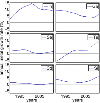
Photovoltaics (PV) have exhibited the most rapid cost decline among energy technologies [4] (Fig. 2-1.) In parallel with cost declines and performance improvement, global PV deployment has grown rapidly [5]. Continued PV deployment could help reduce greenhouse gas emissions and other pollution from energy systems [10], and contribute to climate change mitigation [4]. For PV deployment to experience sustained growth in the future, however, particularly when considering the additional costs of addressing solar intermittency [11], further cost declines are likely needed [12]. This paper aims to identify the causes of PV’s rapid cost declines in the past and gain insight into maintaining the pace of improvement in the future. More fundamentally, we aim to advance a model for understanding the mechanisms of technology improvement at multiple levels, from human efforts to devices, that can be applied to many technologies and measures of performance.

Improvement trends in PV and other technologies have been studied by various research communities. Correlational analysis is a common approach in these studies, often focusing on cost (or other measure of performance) and production or research investment levels [29]. One of the most widely-used models is the experience curve, which relates a technology’s cost to cumulative production as a power law. Using this relationship as an explanatory or predictive tool, studies have estimated the rates of performance improvement for a range of technologies [30, 31, 32, 29, 33]. For example, PV module costs fell by about 20% with every doubling of cumulative capacity since the 1970s [34, 8]. Several explanations for this cost decline have been proposed, such as public research and development efforts and various consequences of market growth [7], including learning-by-doing, economies of scale, and private research and development efforts [35, 36, 34, 37, 38]. These studies share an approach to examining technology cost evolution where important high-level drivers of cost reduction are assumed and their influence on cost is inferred based on correlation. Technologies are treated as black boxes and the causes of cost reduction within technology are not modeled mechanistically.

Another group of studies uses detailed, device-level cost models, to understand how features of a technology or manufacturing process contribute to costs at one or more snapshots in time. Several such studies exist for PV, and they provide information on how individual cost components contribute to total costs, while taking into account the physics of PV

(23)

years 1975 1980 1985 1990 1995 2000 2005 2010 2015 2015$/W 1 10 100 price, Reichelstein

cost, China, Pillai cost, other countries, Pillai cost, Pillai price, Pillai price, Maycock price, Swanson cost, Ravi price, Ravi cost, Mints price, Mints cost, Christensen cost, Christensen cost, Maycock price, Nemet cost, Powell cost, China, Goodrich cost, US, Goodrich price, Feldman

Figure 2-1: Costs are shown in orange, and prices are shown in purple. References: Reichel-stein [71], Pillai [72], Maycock price data from [8] and cost data from [73], Swanson [74], Ravi [75], Mints [9], Christensen [76], Nemet [8], Powell [41], Goodrich [77], Feldman [78]. Values are averages across different PV technologies except for those in Powell [41] (multicrystalline silicon) and Goodrich [77] (monocrystalline silicon). Differences across datasets show the effect of sampling errors.

technologies [40, 41, 42, 43, 15]. They also propose avenues for future technical improvement at the device or manufacturing level, and estimate cost reductions that might be achieved in the future [79]. Missing from these studies, however, is a method of accurately quantifying how each change to a feature of the technology or manufacturing process contributes to cost reductions, when many changes occur simultaneously. This knowledge is needed to understand the mechanisms of cost reduction but requires further modeling advances.

Pursuing both dynamic and detailed, device-level models is critical for identifying the causes of improvement in PV and other technologies. This combined approach would address inherent limitations in using correlational analyses to identify causal effects, especially in the case where data is limited, as is often the case in technology evolution research. This approach would also address the lack of dynamics in device-level studies. A few past studies have begun to develop such a methodology by decomposing technology costs over time [8, 44]. A study of the drivers of PV module cost changes from the 1970s to the early 2000s [8] pioneered a bridge of this kind, and found that learning-by-doing had a limited effect on cost reductions.

(24)

In this paper we propose a new conceptual framework and dynamic-yet-detailed quanti-tative model for analyzing PV’s (or any technology’s) cost evolution. We start with a cost equation that computes costs from a set of explanatory variables, such as module efficiency, wafer area, and manufacturing plant size. From this we derive cost change equations that estimate the contribution of each variable to cost changes. Since multiple simultaneous changes to variables have different impacts on cost than individual changes summed together, attributing cost changes to individual variables is challenging. Our method of estimating variable contributions is based on adapting calculus derivative formulas to finite differences.

In attributing PV’s cost decline to particular causes, we draw a distinction between low-level causes (or mechanisms) and high-low-level causes (or mechanisms). Low-low-level mechanisms explain cost reduction in terms of changes to particular variables of a cost model. High-level mechanisms explain cost reduction in terms of processes like public and private R&D, learning-by-doing, and scale economies that can influence technology costs in less specific ways. High-level mechanisms are discussed widely in studies of historical technology evolution.

By considering both the low-level and high-level causes of PV’s improvement we uncover lessons that are useful for a variety of decision-makers. These may include engineers who design and manufacture PV modules, or firm managers and government policy-makers who develop strategy to support technological development. For example, our findings contribute to a long-standing debate concerning the effect of public investments in R&D versus market-expansion policies [31, 69, 70].

We focus on crystalline silicon PV modules because of their long history and dominant market share among PV technologies [80]. Since the 1950s, this technology has improved steadily due to R&D and manufacturing efforts [40]. We analyze the costs starting in 1980, when space applications of PV were overtaken by terrestrial applications, which did not require as high quality and reliability [81, 8, 82]. We look at typical costs globally, since PV modules are manufactured and traded globally. The method we develop can be adapted to study PV systems as a whole (including non-module cost components that show significant potential for cost reduction [83, 84]), and a wide range of other technologies and measures of performance other than cost [85, 10, 86]. The method might also prove a useful quantitative framework for eliciting high-quality input from experts on the prospects for future technological improvements [87].

(25)

model. Section 2.3 explains the method of attributing cost changes to variables. Section 2.4 shows the results of our analysis and the connection between low-level and high-level mechanisms. In Section 2.5 we discuss the implications for future developments in PV and conclude.

2.2 Cost model

We first develop a cost model for PV modules. The cost components are calculated based on quantities (or usage ratios) 𝜑 and prices of inputs 𝑝 used in manufacturing.

𝐶𝑚 (︂ $ 𝑚𝑜𝑑𝑢𝑙𝑒 )︂ = 1 𝑦𝑚 ∑︁ 𝑖̸=𝑐,𝑤 𝜑𝑚𝑖𝑝𝑖 ⏟ ⏞

non-cell module costs

+ 𝑛𝑚𝑐 𝑦𝑚𝑦𝑐 ∑︁ 𝑖̸=𝑤 𝜑𝑐𝑖𝑝𝑖 ⏟ ⏞

non-wafer cell costs

+𝑛𝑚𝑐𝑛𝑐𝑤 𝑦𝑚𝑦𝑐𝑦𝑤 ∑︁ 𝑖 𝜑𝑤𝑖𝑝𝑖, ⏟ ⏞ wafer costs (2.1) where

𝑦𝑚 yield at module manufacturing

𝑦𝑐 yield at cell manufacturing

𝑦𝑤 yield at wafer manufacturing

𝜑𝑚𝑖 quantity of input 𝑖 per module

𝜑𝑐𝑖 quantity of input 𝑖 per cell

𝜑𝑤𝑖 quantity of input 𝑖 per wafer

𝑝𝑖 price of input 𝑖

𝑛𝑚𝑐 number of cells per module

𝑛𝑐𝑤 number of wafers per cell.

While this equation has been written to represent wafer, cell, and module costs, which is an decomposition scheme specific to PV, the formulation of costs in terms of usage ratios (𝜑) and input prices (𝑝) is a general one that can describe any technology. 𝜑 variables generally change as the result of engineering efforts to improve efficiency and materials utilization, while 𝑝 variables change due to bulk purchasing, scarcity or other market effects [19], or input substitutions.

At each of the three levels of PV manufacturing costs – wafer production, cell production, and module production (vertical levels in Fig. 2-2) – there are costs for materials, labor,

(26)

module cost cell cost wafer cost Cost of other materials

Plant size dependent costs

Cost of other materials

Silicon cost

Cost of other materials

slurry, wire, crucible electricity, O&M, labor, depreciation electricity, O&M, labor,

depreciation electricity, O&M, labor,

depreciation

aluminum and silver, chemicals glass, frame, backsheet,

junction box, cable

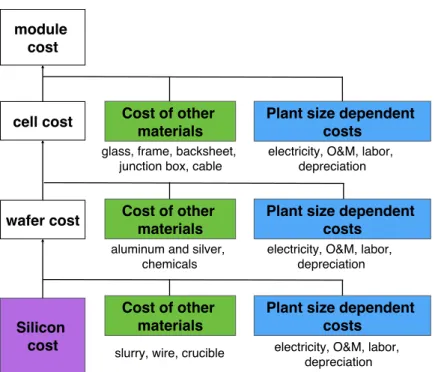
Figure 2-2: Cost components for wafer, cell and module levels (vertical disaggregation) and different input types (horizontal disaggregation).

operation & maintenance, electricity, and depreciation of plant and equipment. Decomposing by level disaggregates the production process for PV modules, but creates challenges here for estimating the sources of cost reduction over time. A consistent categorization of costs is needed for every time period of interest starting with 1980, but such early cost data is scarce. Instead we accomplish this consistency over time by decomposing module production costs into three components by input type: silicon costs, non-silicon material costs, and plant-size dependent costs (horizontal categories in Fig. 2-2). These components are further modeled as described below.

2.2.1 Silicon costs

Historical prices of silicon (i.e. polysilicon) can be obtained from the literature [35, 88, 8] or from industry sources [9]. The amount of silicon used per wafer is a function of wafer area, silicon density, silicon layer thickness, and silicon utilization (the fraction of the silicon ingot used in the wafer after accounting for losses). Multiplying by the number of cells and the price of silion, total silicon cost for the module can be expressed as

Si cost = 𝑛𝑚𝑐

𝐴ℎ𝜌

(27)

Factor Unit 1980 2001 2012

Plant size (𝐾) MW/yr 0.125 14 400

Module efficiency (𝜂) unitless 8% 13% 15%

Polysilicon price (𝑝_𝑠) 2015$/kg 66 32 21

Wafer area (𝐴) cm2 80 150 243

Silicon usage (𝑣) ≡ thickness (𝑡)/utilization (𝑈 ) cm 0.25 0.07 0.04

Yield (𝑦) unitless 75% 88% 95%

Share of materials costs (𝜃) unitless 0.58 0.43 0.65

Scaling factor (𝑏) unitless 0.27 0.27 0.27

Module cost 2015$/W 22.1 4.1 1.3

References: Plant size: 2012 [9, 41]. Module efficiency: 1980 [8, 9]. Silicon usage: 1980 [89, 8], 2001: [90, 8], 2012: [41]. Share of materials costs: 1980: [91], 2001: [73], 2012: [41]. Scaling factor: all years [73]. Other values shown in the table are obtained from [9].

Table 2.1: Data used to calculate module cost components.

Here 𝑛𝑚𝑐 is the number of cells per module, 𝐴 is wafer area, ℎ is wafer thickness, 𝜌 = 2.33

g/cm3 is wafer density, 𝑈 is silicon utilization, and 𝑝_𝑠 is the price of polysilicon. We define the combination 𝑣 ≡ ℎ/𝑈 , which we refer to as ‘silicon usage’ for simplicity. The data for these variables are provided in Table 2.1.

2.2.2 Non-silicon materials costs

Non-silicon materials include the crucible used to produce silicon ingots; slurry and wire used for wafer-sawing; aluminum and silver pastes, chemicals and screens used in cell manufacturing; and glass, frame, backsheet, encapsulant, ribbon, junction box and cable used in the module [41]. To a first-approximation, the usage of these materials can be categorized as proportional to wafer area (e.g. aluminum pastes), proportional to module area (e.g. glass), proportional to module perimeter (e.g. frame), or neither (e.g. junction box), so that costs would take the form

non-Si materials costs = 𝑐0+ 𝑛𝑚𝑐𝑐1𝐴 + 𝑐2𝐴𝑚+ 𝑐3𝑃 (2.3)

with 𝐴 representing wafer area, 𝐴𝑚 the module area, 𝑃 the module perimeter, and the 𝑐𝑖

various constants. Because of data limitations, and since most materials costs depend on area, we ignore the fixed and perimeter dependent categories in this expression. Since the

(28)

late 1970s wafer area 𝐴 and module area 𝐴_𝑚 have increased proportionally,2 𝐴 ∝ 𝐴𝑚. Thus

we simplify Eq. (2.3) to

non-Si materials costs = 𝑛𝑚𝑐𝑐𝐴, (2.4)

where 𝑐 is the per-area cost of all non-silicon materials and 𝐴 is wafer area. Here the non-Si materials costs account for the costs at all of the wafer, cell and module levels. We derive the value of 𝑐 from estimated materials costs in the three time periods. Based on the literature, the share of materials costs in PV modules varied between 35-65% [73, 41]. We calculate the materials costs using the total module cost and the fraction due to materials, subtract the cost of silicon, and divide out the wafer area to obtain 𝑐.

2.2.3 Plant size-dependent costs

We assume that electricity, labor, maintenance and depreciation costs per wafer varies with the plant size due to scale economies. We model this group of costs as

plant size-dependent costs = 𝑛_𝑚𝑐𝑝0

(︂ 𝐾 𝐾0

)︂−𝑏

, (2.5)

where 𝐾₀ is a reference plant size, 𝑝₀ represents the total of these costs for a plant with the reference size, and 𝑏 is the scaling factor. For convenience we take 𝐾0 = 400 MW (the value

for 2012), though this choice is just a convention since the effects of a different choice of 𝐾0 would be absorbed into a different value for 𝑝0. We use 𝑏 = 0.27 as the scaling factor

[73]. We obtain this value by computing the change in labor, capital, utilities and overhead costs between plants of two sizes described in [73]. We obtain 𝑝0 for 2012 from [41]. For

1980 and 2001 we compute 𝑝₀ by computing non-materials costs and dividing out the factor (𝐾/𝐾0)−𝑏.

2

The relationship between wafer area and module area is given by

𝐴module= 𝑛𝑚𝑐𝐴

𝛼

where 𝑛𝑚𝑐is the number of cells per module and 𝛼 is the area utilization, the fraction of module area used by cells. Both wafer area and module area increased about three-fold in the last twenty years, while 𝛼 and 𝑛𝑚𝑐 have stayed almost constant in a typical module [76, 41].

(29)

2.2.4 Final cost equation

The power output of a module 𝐾𝑚 is given by

𝐾𝑚 =

𝜎𝑛𝑚𝑐𝐴𝜂

𝛼 (2.6)

where 𝜎 = 0.1 W/cm2 is the solar constant, 𝑛𝑚𝑐 is the number of cells per module, 𝐴 is

wafer area, 𝜂 is module efficiency, and 𝛼 is module area utilization. We assume a constant value of 𝑛𝑚𝑐 = 72. Summing the three components of module costs, and dividing by module

capacity, total costs are

𝐶(︂ $ 𝑊 )︂ = 𝛼 𝜎𝐴𝜂𝑦 [︃ 𝐴𝑣𝜌𝑝𝑠+ 𝑐𝐴 + 𝑝0 (︂ 𝐾 𝐾0 )︂−𝑏]︃ . (2.7)

Some wafers, cells, and modules created during production are faulty and must be discarded, leading to waste and additional costs. To account for this we include the production yield 𝑦 above.3 We populate Eq. (2.7) with historical data from three snapshots in time: 1980, 2001 and 2012 (Table 2.1). Theoretically one could model all of the cost components including the materials, electricity, labor and so on as dependent on both plant size and wafer area. However, the data to populate such a sophisticated model is not available. Therefore we make a compromise and model the electricity, labor, maintenance and depreciation costs as scaling with plant size, while we model materials costs as dependent on wafer area.

Using the cost equation and the data in Table 2.1, we obtain the three cost components for 1980, 2001 and 2012. The cost components are illustrated in Fig. 2-2 and their values are shown in Table 2.2. While all of the cost components have gone down in units of $/W, their shares of total cost have varied. In particular silicon has became a smaller fraction of total cost over time, while non-silicon materials have become a larger fraction. The share of the plant-size dependent costs increased between 1980 and 2001 and then decreased after 2001. Our decomposition variables are similar to [8] (and one of the time periods we consider (1980-2001) is the same as in [8]), though there are a few important differences which are summarized here. We include the contribution of non-silicon material costs, which are not considered in [8]. To avoid double-counting the reductions from efficiency improvements, we model silicon usage in units of g/module instead of g/W. Similarly we model plant 3_{Wafer, cell and module production each have individual process yields, though for simplicity we represent} overall yield with one value.

(30)

Cost component 1980 2001 2012

2015$/W Percentage 2015$/W Percentage 2015$/W Percentage

Silicon cost 5.70 26% 0.41 10% 0.12 9%

Non-silicon materials cost 7.14 32% 1.34 33% 0.72 55%

Plant size-dependent cost 9.29 42% 2.33 57% 0.46 35%

Total module cost 22.13 4.08 1.30

Table 2.2: Cost components in 1980, 2001 and 2012. Total module costs are obtained from [9].

output in units of modules/year instead of W/year. The share of costs that we find to be plant size-dependent and area-dependent are different. In [8], all costs are modeled as being plant-size dependent while we model only non-materials costs as plant-size-dependent, based on [73]. Also based on [73] we use a higher exponent for scale-dependent costs, 𝑏 = 0.27 versus 𝑏 = 0.18 in [8]. Therefore, compared with [8] our plant scale variable affects a smaller fraction of total module costs, while influencing this fraction more strongly. We similarly model all materials costs as area-dependent, and all non-materials costs as non-area-dependent. As a result a much larger fraction of costs are independent of wafer area in our model, 35-60% depending on the period versus 4% in [8]. Other differences in the modeling approach used here and in [8] are discussed at the end of Section 2.3.

2.3 Attributing cost changes to variables

How much of the cost reduction in PV modules came from each variable in Eq. (2.7)? Here we outline a general approach for computing these contributions from an equation for costs, with the derivation given in the SI. Identifying the determinants of a change in technology costs is more challenging than obtaining snapshots of cost components over time for two reasons. First, one must unravel the network describing how cost components (e.g. non-silicon materials costs) depend on input variables (e.g. wafer area). A second challenge is to decompose cost changes in discrete time.

To address these challenges, we first write down (through knowledge of a technology) an equation for cost as a function of a vector of explanatory variables (EVs):

𝐶(r𝑡) =∑︁

𝑖

(31)

𝐶 is the cost of the technology and r𝑡 is the vector of EVs at time 𝑡. The total cost is a sum over several cost components 𝑐𝑖 that depend on the EVs. Often the cost components can be

written as products of functions of the EVs, as is the case with Eq. (2.7), so that we can write

𝑐𝑖(r𝑡) = 𝑐𝑖0

∏︁

𝑗

𝑔𝑖𝑗(𝑟𝑗𝑡) (2.9)

where 𝑔𝑖𝑗(𝑟𝑗𝑡) gives the dependence of the 𝑖th cost component on the 𝑗th variable. The

prefactor 𝑐_𝑖0 combines any other constants that do not depend on the EVs. In the SI we show that the change to total cost is approximately

∆𝐶 ≈∑︁ 𝑗 (︃ ∑︁ 𝑖 ˜ 𝑐𝑖∆ ln 𝑔𝑖𝑗 )︃ ≡ ∆𝐶approx, (2.10)

where ˜𝑐𝑖 ≡√︀𝑐𝑖(r1)𝑐𝑖(r2) is the geometric average of the cost component 𝑖 in the two time

periods, and ∆ ln 𝑔_𝑖𝑗 = ln 𝑔𝑖𝑗(𝑟𝑗2) − ln 𝑔𝑖𝑗(𝑟1𝑗). Eq. (2.10) implies that the contribution of the

𝑗th variable is ∆𝐶𝑗 = ∑︁ 𝑖 ˜ 𝑐𝑖∆ ln 𝑔𝑖𝑗. (2.11)

Eq. (2.11) provides an estimate of how much cost reduction the 𝑗th variable is individually responsible for.

In our case, the EVs are r𝑡= (︀𝐴𝑡_{, 𝜂}𝑡_{, 𝑦}𝑡_{, 𝐾}𝑡_{, 𝑝}𝑡

𝑠, 𝑣𝑡, 𝑐𝑡, 𝑝𝑡0)︀. The cost components in Eq.

(2.7) can be written in the form of Eq. (2.9) as

𝑐1(r) = (︁𝛼𝜌 𝜎 )︁ 𝑣𝑝𝑠𝜂−1𝑦−1 (2.12) 𝑐2(r) = (︁𝛼 𝜎 )︁ 𝑐𝜂−1𝑦−1 (2.13) 𝑐3(r) = (︃ 𝛼 𝜎𝐾₀−𝑏 )︃ 𝑝0𝐾−𝑏𝐴−1𝜂−1𝑦−1, (2.14)

which are (from top to bottom) silicon costs, non-silicon materials costs, and plant-dependent costs. Then Eq. (2.11) can be computed to form the estimates for individual variables. For

(32)

example, the module cost change due to the change in efficiency is ∆𝐶𝜂 = 3 ∑︁ 𝑖=1 ˜ 𝑐𝑖∆ ln 𝜂−1 = [︃ ₃ ∑︁ 𝑖=1 √︀ 𝑐𝑖(r1)𝑐𝑖(r2) ]︃ (︂ ln𝜂 1 𝜂2 )︂ . (2.15)

To complete the approach, we make one final modification to Eq. (2.11). ∆𝐶 is a non-linear function of variable changes ∆𝑟_𝑗; however, ascribing portions of ∆𝐶 to particular variables necessarily means making a linear approximation. This in turn means that the sum over ∆𝐶𝑗 (i.e. ∆𝐶approx) can be greater or less than the actual change in cost ∆𝐶. Our goal

is to score the relative importance of different EVs, not to characterize the non-linearity of ∆𝐶, so in computing the contributions of EVs we normalize Eq. (2.11) as follows:

∆𝐶_𝑗norm = ∆𝐶

∆𝐶approx

∆𝐶𝑗. (2.16)

This normalization guarantees that the sum over ∆𝐶_𝑗normsum to ∆𝐶, and percentages based on ∆𝐶_𝑗norm sum to 1.

An important departure from the method of [8] is that we start with a cost equation first rather than beginning directly with cost change equations. This two-step approach has significant advantages. It ensures that our cost change equations are consistent with a realizable cost model, whose values can be directly compared with actual costs. A cost model shows explicitly how variables jointly determine total cost, making it easier to see what modeling assumptions are being made. It also helps to avoid double-counting or undercounting the effects of explanatory variables on costs, because the dependence of cost on each variable has been fully accounted for in the cost model.4

4_{As an example of how double-counting can occur, silicon usage in PV modules is sometimes expressed in} units of grams per watt. However, silicon usage per watt can decrease either because of a reduced silicon need per wafer, or because of an efficiency improvement. Efficiency of PV modules improved at the same time that silicon needs per wafer decreased. As a result, silicon usage per watt has changed more than silicon usage per wafer has. If the full cost reduction benefit of higher efficiency were already counted elsewhere, then the silicon-usage benefit of higher efficiency will be double-counted.

Double-counting is less likely to occur if the analysis of cost changes starts with an equation for cost. In constructing this equation, the grams-per-watt units of silicon usage would have to be reconciled with the watts units of efficiency × wafer area × the solar constant to recover the correct units for cost. Once this reconciling of units is done, the cost change equations that are derived from the cost equation will automatically avoid double-counting as well.

(33)

1980-2001 % contribution to module cost change -10 0 10 20 30 ∆ p0 ∆ Silicon price ∆ Yield ∆ Plant size ∆ Silicon usage ∆ Wafer area ∆Non-Si materials costs ∆ Efficiency

2001-2012 % contribution to module cost change -10 0 10 20 30

Overall (1980-2012) % contribution to module cost change -10 0 10 20 30

Figure 2-3: Contribution of the low-level mechanisms to module cost decline in 1980-2001 (left), 2001-2012 (middle), and 1980-2012 (right). Mechanisms are listed in the order of

decreasing contribution for the 1980-2001 period.

2.4 Results and discussion

In this section we first discuss the low-level mechanisms of module cost reduction, which refer to changes to variables in the cost equation. We then relate the low-level mechanisms to high-level mechanisms of cost reduction, which refer to processes at the level of institutions arising from human efforts.

2.4.1 Low-level mechanisms of cost reduction

Figure 2-3 and Table 2.3 show the changes in module cost due to each variable in the two periods, 1980-2001 and 2001-2012, and the entire period, 1980-2012. Improving efficiency was the largest contributor in the first period, responsible for 29% of the cost reduction. In the second period, module efficiency was only the fourth most significant factor, and its contribution dropped to 13%. Efficiency increased at the wafer and cell levels through many improvements, such as surface passivation [81], anti-reflective coating [92], and texturing of the wafers [93, 94], and at the module level with improvements such as a glass structural layer laminated design [81].

(34)

Cost change due to: 1980-2001 2001-2012 1980-2012 ∆2015$/W Percentage ∆2015$/W Percentage ∆2015$/W Percentage

∆ Efficiency -5.20 29% -0.35 13% -5.55 27%

∆ Non-Si materials costs -3.66 20% -0.43 15% -4.09 20%

∆ Wafer area -3.37 19% -0.54 20% -3.92 19% ∆ Silicon usage -2.22 12% -0.14 5% -2.36 11% ∆ Plant size -2.04 11% -0.86 31% -2.90 14% ∆ Yield -1.71 9% -0.19 7% -1.90 9% ∆ Silicon price -1.28 7% -0.10 4% -1.39 7% ∆ p0 1.45 -8% -0.17 6% 1.28 -6%

Change in module cost -18.05 100% -2.78 100% -20.83 100%

Table 2.3: Contribution of the low-level mechanisms to module cost decline in 1980-2001 (left), 2001-2012 (middle), and 1980-2012 (right). Mechanisms are listed in the order of decreasing contribution for the 1980-2001 period. Cost changes due to the low-level mechanisms and their percentage contributions are normalized as explained in Eq. 2.16 in Section 2.3.

The second most significant factor in 1980-2001 was lower per wafer area costs of non-silicon materials, contributing 20% of the cost decline. The contribution of this factor in 2001-2012 was 15%. Non-silicon materials include substances such as as glass, laminate, and metal paste that become embedded in the module as well as slurry and wire used during production. The cost of these materials has been reduced by various process and module design improvements. For example, the cost of slurry used in wafer cutting may be reduced by recycling, with recycling rates up to 80% reported [95].

Increasing wafer area was an important factor in both periods. Wafer area almost doubled from 80 cm2 to 150 cm2 in 1980-2001, and grew significantly again to about 240 cm2 by 2012. A doubling of wafer area, given a fixed number of cells per module, means that each module assembled produces twice as much power. Material costs are mostly proportional to area, but other assembly costs are insensitive to area [96, 8], so that larger wafer area yields cost savings.

Process improvements led to increasing yields in wafer, cell and module production. Overall yield increased from 75% in 1980 to 95% in 2012. The change in yield contributed 9% and 7% to the module cost decline in 1980-2001 and 2001-2012, respectively. Reduced handling of wafers, cells and modules due to automation, and improvements in processes such as wafering, help to increase yield [95]. We note that other improvements (such as larger wafer sizes) can decrease yields [94], so that yield considerations can be a limiting factor for otherwise cost-saving practices.

(35)

on wafer thickness ℎ and silicon utilization 𝑈 . To study the total cost reduction from both variables, we define the combination 𝑣 ≡ ℎ/𝑈 . In 1980-2001 wafer thickness decreased from about 500 𝜇m to 250 𝜇m while silicon utilization increased from about 20% to 35%. Reduced thickness and higher utilization contributed about equally to the silicon cost reduction in this period. Silicon usage continued to decrease in 2001-2012, though it had a less significant cost impact. The industry developed thinner wafers both to reduce the cost of silicon and to increase conversion efficiency [92]. Silicon utilization also increased, though losses remain high, with about 50% of entering silicon lost during slicing of wafers from silicon ingots. Decreasing thickness contributed about 70% of silicon cost reduction in this period while utilization contributed the remaining 30%.

Changes in polysilicon price contributed about 7% and 4% of the module cost decline in 1980-2001 and 2001-2012, respectively. The endpoints of our analysis lie on either side of a temporary period of silicon shortage in 2005-2008, during which polysilicon prices surged. Before this period, most polysilicon was used by the semiconductor industry. The PV industry used wafers rejected by the semiconductor industries, which has higher purity requirements [90]. Around 2006 polysilicon demand by the PV industry surpassed that of the semiconductor industry and polysilicon producers responded by increasing capacity. While more than 80% of the global polysilicon production was consumed by the semiconductor industry before 2000 [97], about 90% went to manufacturing PV cells as of 2012 [98].

The pre-factor 𝑝₀ in Eq. (2.5) provides the level of plant-size dependent costs for a plant of a fixed size 𝐾0, thus accounting for the overall level of electricity, labor, capital and

depreciation costs at each time. The change in 𝑝₀ was estimated to have increased cost in the 1980-2001 period and decreased cost in the 2001-2012 period. As described in Section 2.2 we calibrate 𝑝₀ in 1980 and 2001 by requiring non-material costs in our cost model to match values from our data. We regard the variable with caution since changes are difficult to interpret and it is likely to propagate uncertainty in the data. However, its effects are among the smallest in both periods.

Finally, increasing manufacturing plant sizes resulted in scale economies through shared infrastructure, reduced labor requirements, higher yield, and better quality control [99]. Typical plant sizes have scaled up with the industry, starting from 0.125 MW in 1980 and growing to 14 MW in 2001 and to 400 MW in 2012. Plant size became an especially significant factor in the more recent period, contributing almost a third of the decline in module cost.

(36)

In Section A.2 of the Supporting Information we estimate the sensitivity of our results to the uncertainty in the input variables shown in Table 2.1. We conclude that overall our results are robust to changes in the variables.

Our findings show some similarities to earlier reported results [8], as well as some differences. Similar to [8] we find that the contribution of increasing module efficiency to cost reduction in the 1980-2001 period was around 30%. While [8] finds the sources of cost declines to be heavily concentrated in plant size and module efficiency changes, we find cost-reducing effects were spread across a number of variables. In [8] the costs of non-silicon materials are not considered, though we find that non-silicon material costs contributed as much to cost reduction as silicon did in this period. We obtain a lower estimate for the contribution of plant size in this period (11% versus 46%), and larger contributions for wafer area (19% versus 3%), silicon consumption (11% versus 3%) and yield (9% versus 2%). We find a roughly similar magnitude for silicon price (7% versus 12%).

2.4.2 High-level mechanisms of cost reduction

1980-2001 % contribution to module cost change

0 20 40 60 80

other EOS LBD public and private R&D

2001-2012 % contribution to module cost change

0 20 40 60 80

Overall (1980-2012) % contribution to module cost change

0 20 40 60 80

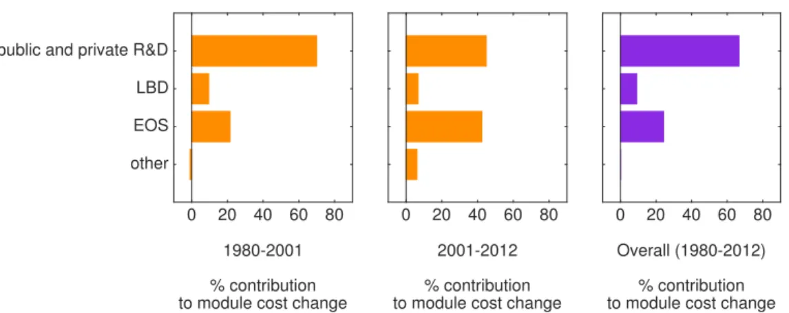
Figure 2-4: Percentage contribution of the high-level mechanisms to module cost decline in 1980-2001 (left), 2001-2012 (middle), and 1980-2012 (right). R&D = Research and develop-ment, LBD = Learning-by-doing, EOS = Economies of scale, Other = other mechanisms such as spillovers. We categorize the changes that require a lab setting or a nonroutine production activity (e.g. experimental production line) as being caused by R&D [100, 101]. We consider an improvement to have been made by LBD if it was achieved as a result of repeated routine manufacturing activity and if it was incremental in nature [100]. Changes that result from increases to the scale of the module manufacturing plant we categorize as EOS.

Low-level cost reductions were driven by various ‘high-level’ mechanisms such as research and development, learning-by-doing, and economies of scale. Estimating the contributions of

(37)

1980-2001 % contribution from market expansion policies

0 20 40 60 80 100 EOS LBD 50% R&D market expansion policies public R&D and other 2001-2012 % contribution from market expansion policies

0 20 40 60 80 100 EOS _LBD 50%_R&D market expansion policies public R&D and other Overall (1980-2012) % contribution from market expansion policies

0 20 40 60 80 100 EOS _LBD 50% R&D market expansion policies public R&D and other

Figure 2-5: Percent contribution of market expansion policies (e.g. feed-in-tariffs, renewable portfolio standards) to module cost reduction in 1980-2001 (left), 2001-2012 (middle), and 1980-2012 (right). Scale economies, learning-by-doing, and private R&D were all stimulated by market expansion. Our data does not let us separate the effects of private and public R&D. To accommodate this, we add 50% of total R&D contributions to the contributions of scale economies and learning-by-doing. This effectively assumes that 50% of R&D improvements came from private R&D (roughly commensurate with the share of R&D expenditures in clean energy [7, 102, 103, 104]). Uncertainty bars show the total contribution from market expansion policies that would result under the alternate assignments of low-level mechanisms to high-level mechanisms shown in Fig. A-12 without accounting for uncertainty in the private R&D estimate.

these mechanisms is useful because they align more closely with the policy levers often used to drive down cost. To estimate how much each contributed to cost reduction in PV modules (Fig. 2-4), we categorize each low-level variable according to which high-level mechanism was most responsible for its change. In Section A.3 of the Supporting Information we perform a sensitivity analysis to test the effect of these assumptions. Our conclusions about the relative importance of different high-level mechanisms are robust to various schemes for relating low-level and high-level mechanisms (see Fig. A-12).

Changes that require a lab setting or a nonroutine production activity (e.g. experimental production line) are labeled as being caused by research and development (R&D) [100, 101]. R&D can result in improvements to either the manufacturing process or the technology being produced. We consider an improvement to have been made by learning-by-doing (LBD) if it was achieved as a result of repeated routine manufacturing activity and if it was incremental in nature [100]. Cost changes that result from increases to the module manufacturing plant scale, and from volume purchases of materials or scale economies in materials supplier industries, we categorize as economies of scale (EOS).

Based on this we categorize improvements to module efficiency, wafer area and silicon usage under R&D. Improvements to cell efficiency were largely achieved by R&D done at national labs, universities and companies. Closing the gap between cell and module

(38)

efficiencies also required R&D to improve module assembly processes such as encapsulation and interconnections. Larger wafer area was achieved through R&D on single crystal growing and multicrystalline ingot casting. Wafer thickness and silicon utilization improved though manufacturing techniques such as wire-sawing that were improved through R&D. LBD may have been an additional driver of wafer area and silicon usage, which are affected by the efficiency of the manufacturing process.

Yield likely improved mainly through LBD, as advances in quality control of wafers and cells reduced rejects and increased automation reduced excess handling. R&D may have played a role, though we expect that improving yield mainly involved repeated routine manufacturing activity.

The increasing size of module plants brought about economies of scale (EOS), as manufac-turers simultaneously prepared for higher demand [8] and looked for better access to capital [77]. Larger plants realized cost savings from spreading out the costs of shared infrastructure across greater output and from physical or geometric scaling relationships [105, 106]. In our model we assume all non-material costs realize scale benefits so that increasing plant sizes lowers the cost per watt of labor, capital equipment, and electricity.

Silicon prices were driven by different developments over time. Until the mid-2000s, demand for silicon wafers by the PV industry was met mainly with wafers rejected by the semiconductor industry. The availability of silicon was a positive externality of semiconductor production and not a result of R&D, LBD, or EOS in the PV industry. We therefore categorize silicon price’s high-level mechanism as ‘other’ for 1980-2001. The PV industry surpassed the semiconductor industry in silicon demand around 2006 [107], leading to a price spike and supply shortage. To maintain supply, the PV industry developed its own production of polysilicon. In this period knowledge spillover and scale economies were important. Know-how of producing single crystal silicon ingots and slicing wafers was acquired from the semiconductor industry by the PV industry, which rapidly scaled-up its own capacity. For 2001-2012 we therefore choose EOS as the main high-level mechanism for decreasing silicon price.

Decreases to non-silicon materials costs were important sources of cost reduction in both time periods. Non-silicon materials costs can be decomposed into material usage (mass/area) times material price (dollars/mass). We propose that R&D helped reduce materials usage through new module designs, while EOS led to the decreasing prices due to volume purchases