HAL Id: hal-00432693
https://hal.archives-ouvertes.fr/hal-00432693
Submitted on 16 Nov 2009
HAL is a multi-disciplinary open access
archive for the deposit and dissemination of
sci-entific research documents, whether they are
pub-lished or not. The documents may come from
L’archive ouverte pluridisciplinaire HAL, est
destinée au dépôt et à la diffusion de documents
scientifiques de niveau recherche, publiés ou non,
émanant des établissements d’enseignement et de
Measurement of the pure dissolution rate constant of a
mineral in water
Jean Colombani
To cite this version:
Jean Colombani. Measurement of the pure dissolution rate constant of a mineral in water. Geochimica
et Cosmochimica Acta, Elsevier, 2008, 72, pp.5634-5640. �10.1016/j.gca.2008.09.007�. �hal-00432693�
Measurement of the pure dissolution rate constant of a mineral in water
Jean Colombani1Laboratoire de Physique de la Mati`ere Condens´ee et Nanostructures, Universit´e de Lyon, F-69003, Lyon, France;
Universit´e Claude Bernard Lyon 1, F-69622 Villeurbanne, France; CNRS, UMR 5586, F-69622 Villeurbanne, France
Revised version - 5 september 2008
Abstract—We present here a methodology, using holographic interferometry, enabling to measure the pure surface reaction rate constant of the dissolution of a mineral in water, unambiguously free from the influence of mass transport. We use that technique to access to this value for gypsum and we demonstrate that it was never measured before but could be deduced a posteriori from the literature results if hydrodynamics is taken into account with accuracy. It is found to be much smaller than expected. This method enables to provide reliable rate constants for the test of dissolution models and the interpretation of in situ measurements, and gives clues to explain the inconsistency between dissolution rates of calcite and aragonite, for instance, in the literature.
1
INTRODUCTION
Among heterogeneous reactions, dissolution of minerals in water is encountered in a wide spectrum of fields, from geochemistry to materials science, soil science, environmental science or oceanography. It plays a leading role, for instance, in the weathering of rocks as much as in the durability of mineral materials, in soils amendment, in pollutant spreading, or in sediment-water interaction. In all these situations, quantitative kinetic models are required to describe the involved phenomena.
More recently, this phenomenon has been recognized as being a keypoint in the modelisation of the atmospheric PCO2 variation. Indeed, among the mechanisms controlling the pH of the ocean, and
influencingin turnthe atmospheric PCO2, dissolution drives two major steps: the weathering of terrestrial
carbonates and the deep-sea sediment-water interaction (Anderson and Archer, 2002). Therefore kinetic models of PCO2 change require reliable in situ and laboratory dissolution rates (Hales and Emerson,
1997).
But the establishment of reliable rate laws faces several difficulties. First, multiple lengthscales, and accordingly timescales, are involved during the dissolution process of a mineral, from the individual atomic detachment to the change of shape of the solid. Secondly, the number of parameters influencing the global dissolution kinetics is particularly large: surface topology, amount and nature of surface defects, adsorbed species, reactive surface area, pressure, temperature, composition of the solution, hydrodynamic behavior of the liquid, pH, . . . So a comprehensive dissolution model is still lacking and experimental results of dissolution rates show inconsistencies (Morse et al., 2007).
To obtain rate laws of the dissolution of minerals in water, two methodologies are employed. In bulk experiments, the concentration of chemical species in stirred water, where a sample dissolves, is measured and the dissolution rate deduced from the time evolution of this concentration. In local experiments by Atomic Force Microscopy(AFM)or Vertical Scanning Interferometry(VSI), the evolution of the surface topology at the molecular scale is followed during dissolution and the kinetics possibly deduced from atomic step velocity or surface-normal retreat measurement (Vinson and Luttge, 2005). Agreement
between bulk and local techniques remains scarce (cf. Arvidson et al. (2003) for the case of calcite, Luttge et al. (2003) for dolomite, Luttge (2006) for albite and Jordan et al. (2007) for magnesite).
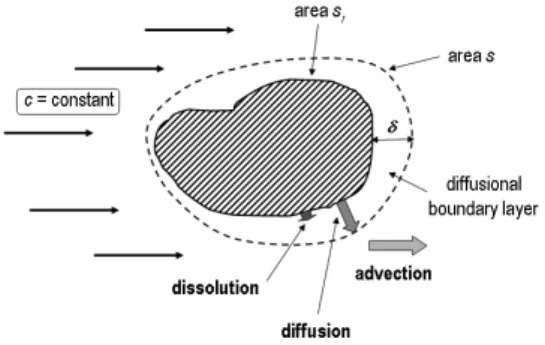
In both experiments the solvent is flowing past the mineral surface, in a laminar or turbulent regime. A mass transport boundary layer develops in the vicinity of the solid, in which the liquid velocity grows from zero at the interface (the no-slip condition), to its bulk value. In this context, dissolution proceeds through three steps (cf. Fig. 1). First the ions are unbound from the solid and solvated. Following a transition state theory the kinetics of the matter removal from the surface obeys a power law Rdiss= ks(1−cs/csat)n, where Rdiss is the dissolution rate, ks the surface reaction rate constant, cs the concentration of the dissolved species at the surface, csat their solubility and n a constant (Lasaga, 1998). Then the ions migrate through the diffusional boundary layer (DBL). The concentration is generally considered as linear in this layer and Fick’s law writes Rdiff = kt(cs−c), where Rdiff is the diffusion rate, kt= D/δ a transport rate constant, D the diffusion coefficient of the dissolved components, δ the DBL thickness and c the concentration in the bulk liquid (Lasaga, 1998). Finally the ions are advected by the flow toward the concentration measurement device. The kinetics of the phenomenon is driven by the slowest step, so minerals are classified according to their transport-controlled (e.g. rock salt), when Rdiff ≪ Rdiss, or reaction-controlled (e.g. quartz), when Rdiff ≫ Rdiss, character. Carbonate and sulfate minerals are considered to belong to a mixed kinetics class where both the transport and reaction flow rates are comparable (Jeschke et al., 2001; Rickard and Sj¨oberg, 1983).
When mass transport is identified as the limiting step, the pure dissolution coefficient ksis inaccessible and only kt= D/δ is obtained in bulk experiments. Though this transport coefficient has been measured in numerous dissolution studies and is sometimes relevant for the understanding of dissolution scenarii in the field or in industrial situations, it does not concern, from a conceptual point of view, the nature of the mineral and the physicochemistry of its surface: the boundary layer depth δ is a pure hydrodynamical quantity and the diffusion coefficient value of the common ions is always D ∼10−9 m2 s−1. For mixed kinetics studies, also largely common, with the help of the above laws, an empirical surface rate constant k can be obtained ”function of both surface reaction and mass transport” (Jeschke et al., 2001), which is different from ks, whereas only this coefficient contains the chemistry of water-mineral interactions and varies by orders of magnitude from minerals to others.
In this paper, (i) we recall that the kinetics of matter removal during dissolution is characterized by a pure surface reaction rate constant, independent of the concentration field in the liquidand of the transport kinetics from the surface to the bulk liquid, and (ii) we claim that this pure dissolution rate constant can be measured unambiguously, even for transport-controlled and mixed kinetics, provided that the concentration field above the surface is known. To ascertain this claim, we have followed the subsequent procedure. First a working mineral and a relevant experimental technique have been selected (Section 2). Then reliable measurements of the pure surface reaction rate constant of this mineral have been performed in conditions where mass transport is proven to have no influence (Section 3). Subsequently most of the experimental dissolution rates available in the literature have been critically collected (Section 4). Finally the validity of these measurements and of our results is discussed (Section 5)
2
MATERIAL AND METHOD
To be able to measure the pure dissolution coefficient without ambiguity, i.e., without needing hydrody-namical assumptions, we need (i) to observe dissolution in absence of any convective flow and (ii) to access to the concentration field in the liquid soaking the solid. To achieve these two goals, we have carried out holographic interferometry measurements of the dissolution of a gypsum single crystal in water at rest.
Holography proceeds in two steps. First the hologram of an object is recorded by enlightening a photographic plate with both the beam coming from the object and a known reference beam. Whereas a classical photograph, where the plate is only enlightened by the object beam, exclusively contains
infor-mations about the light amplitude, the interference pattern of the object and reference beams contains informations about both the amplitude and the phase. The phase itself is linked to the optical path, so to the third dimension and to the refractive index of the object. Secondly the hologram is enlightened only by the reference beam. This one is diffracted by the recorded interference pattern, which gives birth to a three-dimensional image of the object.
Here we use the potentiality of holography to record phase objects, i.e., transparent objects exhibiting only variation of their index of refraction (a transparent liquid, in our case). We record first the three-dimensional state of the studied system in a hologram at time t0. Subsequently we enlighten both the hologram with the reference beam —which creates a 3D image of the object at t0— and the object. Thereby we have a superposition of the object at time t and of this object at time t0. If a variation has occurred between these two times, of concentration for instance, it is visualized through interference fringes. Holographic interferometry differentiates from classical interferometry in the fact that no external reference is needed, the object interfering virtually with a memory of itself.
In the course of an experiment, the hologram of a thermostated optical cell filled with pure water is registered. Then a thin mineral sample is introduced in the cell at a time considered as the time origin t0. Subsequently both the object and the hologram are enlightened and their interference pattern is recorded periodically as shown in Fig. 2. As the mineral dissolves the concentration of the dissolved species in water evolves, so does the refractive index, and the resultant optical path length difference between the object at time t and time t0(recorded in the hologram) induce interference fringes. From the topography of these fringes, the two-dimensional concentration field in the cell can be deduced. Parallely second Fick’s law has been resolved with a first order chemical reaction at the solid-liquid interface in a semi-infinite one-dimensional approximation and brings the concentration evolution c(z, t) with vertical dimension z and time t. The best fit of the experimental curves deduced from holographic results with this analytical expression brings the pure surface reaction rate constant ks. Details on the experimental setup, procedure and data analysis have been given elsewhere (Colombani and Bert, 2007).
To validate our assertionon the hydrodynamical bias present in classical dissolution measurements, we need a mineral with the following requirements. First its dissolution rate must give a discernable amount of dissolved matter in laboratory times. Secondly, its kinetics must be either transport-controlled or mixed. Thirdly the chemical reaction must be as simple as possible, to focus on the hydrodynamical and topological aspects of dissolution. We have therefore discarded calcite, although most effort on mineral dissolution in water has concerned this mineral, because the various steps of the reaction make its kinetic law complex and strongly dependant on the pH and PCO2 values during the experiments.
Gypsum (CaSO4, 2H2O) has been chosen because it fulfills these three criterions and because numerous literature results are available. Beside these methodological considerations, we must notice that gypsum dissolution liberates Ca2+, a cation liable to fix CO
2, and is consequently of importance for the geological sequestration of this greenhouse gas.
3
RESULTS
We had measured the dissolution coefficient of the cleavage plane of gypsum from the Mazan quarry (France), in the frame of a study presenting the possibility of performing mineral dissolution measurement by holographic interferometry (Colombani and Bert, 2007). This work was focussed on the experimental protocole and the cleaved Mazan gypsum sample was studied as an example. Our primary goal here
is the demonstration of the experimental bias introduced by the liquid flow in the classical dissolution experiments (by solution chemistry or local probe). But one difficulty to confront the literature measure-ments and ours lies in the fact that the mineral geometrical and chemical properties differ from one setup to another. In global studies, samples are often powders, sometimes compacted, or polished crystals,
whereas we use cleaved single crystals. So when only one identified interface dissolves in our case, disso-lution in literature stems from multiple crystalline planes separated by steps and kinks. Furthermore the
gypsum origin (so the impurities) differ between experiments. The only sample studied in our preceding work is therefore not sufficient to estimate the dispersion induced by this variation of gypsum samples.
To capture the influence of these differences on ks we have compared some samples to our reference one, i.e., the (010) cleavage plane of gypsum from the Mazan quarry at 20.00◦C (ks= (4 ± 1)×10−5mol m−2 s−1) (Colombani and Bert, 2007). We have carried out holographic interferometry experiments of the dissolution of gypsums of two other quarries: Tarascon-sur-Ari`ege in France (ks= 4×10⁻⁵mol m−2 s−1) and Mostaganem in Algeria (ks= 7×10⁻⁵ mol m−2 s−1) and a synthetic commercial one from MaTeck GmbH (ks = 3×10⁻⁵ mol m−2 s−1), to check the influence of the origin. Then we have carried out experiments with the (120) plane of Mazan gypsum polished with silicon carbide paper of grit size down to 15 µm (ks= 7×10⁻⁵mol m−2 s−1), to evaluate the behavior of non-cleaved planes.
All of these measurements deserve their own study and they were performed here only to estimate the variability of ks in various experimental conditions. But, as a first approach, we can notice that the
dispersion among the ksof the (010) samples of various origins (ks= 3 to 7×10⁻⁵mol m−2s−1) is greater
than the standard error deduced from seven measurements on the (010) Mazan sample in our preceding work (∆ks = 1×10⁻⁵ mol m−2 s−1). The choice of the quarry has therefore a non negligible influence
on the dissolution rate constant. The (010) and (120) planes have different chemical and topological characters. The first one shows originally only water molecules and tends to be atomically flat (Fan and Teng, 2007) whereas the second one is rough and exhibits water molecules, cations and anions. But despite these differences, there is less than a factor of two between their dissolution coefficients.
We are just searching for a ks range representative of the ks encountered in all the samples of the
literature (cf. Section 5) so no average value was computed. Instead, if kmax
s and kmins are the maximum and minimum values, the nominal value of ks has been chosen as (ksmax+ kmins )/2 = 5 × 10⁻⁵ mol m−2 s−1 with an uncertainty of (kmax
s −ksmin)/2 = 2 × 10⁻⁵ mol m−2 s−1.
4
LITERATURE ANALYSIS
Dissolution rates of gypsum in water have been measured for various purposes (karst formation, soil amendment, marine biology, . . . ) and we have tried to gather and analyse these measurements to obtain a coherent view of the literature data. Fig. 3 collects the dissolution rates as a function of calcium concentration of most of the literature results. These include batch (dissolution in a reactor with stir-rer), rotating disk, shaken tube, mixed reactor (rotating disk + flowing liquid) and flume experiments. Unfortunately flowing cell results could not be exploited because dissolution occuring all along the cell, a fixed concentration could not be ascribed to the value of the dissolution rate at the output of the cell (Kemper et al., 1975; Keren and O’Connor, 1982). Gypsum dissolution has been also widely used in ma-rine biology to estimate biological objects interaction with water. But as was extensively demonstrated by Porter et al. (2000) hydrodynamic conditions are often badly or wrongly defined in these studies and dissolution rates cannot be ascribed to unamibiguous concentration and DBL thickness values.
In all these studies, the solvent is pure water and the working temperature is either 20 or 25◦C.
The pH and ionic strength values are almost never given. But despite this lack, the gypsum solubility obtained in all these works is always csat ≈15 mmol l−1, identical to the reference value deduced from
literature analysis by Christoffersen and Christoffersen (1976) or Raju and Atkinson (1990). This proves the proximity between the chemical conditions of these experiments, and gives confidence in the possibility of comparing their dissolution rates.
At first glance, all these measurements do not provide a consistent description of the dissolution of gysum in water (cf. Fig. 3). Up to now, attention has been paid before all to the exponent of the power law of R(c) —considered as representative of the kinetics—, the prefactor being ascribed to the specificities of each experiment. But a correct consideration of the hydrodynamical condition of each device should bring a consistent and predictive knowledge of the dissolution process, whatever the experimental setup. So, first of all, we do not postulate that experiments are either transport-controlled of reaction-controlled
and we make the assumption that all of them are influenced by both chemical reaction and diffusive transport in a variable proportion. The systems are always carefully maintained in a quasi-steady state, where the concentration is uniform in the whole bulk liquid and evolves slowly. So keeping in mind the dissolution steps shown in Fig. 1, we consider that matter is conserved during migration in the diffusional boundary layer. We apply mass conservation between the bottom and top of the DBL, equalizing the dissolution flow rate srRdiss and diffusion flow rate sRdiff:
sDcS−c
δ = srks(1 − cs csat
) (1)
with sr the reacting surface area and s the outer surface area of the DBL (similar to the so-called geometric surface area of the solid, cf. Fig. 1). We have followed Jeschke et al. (2001) and considered that n=1 in Rdiss. From this equation, we compute the only unknown parameter, the surface concentration cs, and we can write the experimental dissolution rate R = Rdiff measured far from the solid after being advected: R = s 1 srks + δ Dcsat − 1 scsat srks + δ D c (2)
The δ = 0 situation reflects an hypothetical absence of DBL where the kinetics is directly driven by the reaction, the transport time between the surface and the measurement device becoming negligible. We see that the pure surface reaction rate constant ks can be accessed via limδ→01/(∂R/∂c) = scsat/(srks). For this purpose, we need an evaluation of csat, δ and s/sr. The solubility is known for long: csat = 15 mmol l−1 (Raju and Atkinson, 1990). The diffusional boundary layer thickness wrapping the dissolving solid for each device is more delicate to obtain This quantity is clearly identified in rotating disk experi-ments: δ = 1.61D1/3ν1/6ω−1/2 with ν the kinematic viscosity of the solution and ω the angular velocity of the disk (Barton and Wilde, 1971). For batch experiments, we have considered that at first order the liquid develops a layer as if flowing past a semi-infinite plate: δ = (2π/0.244)1/3ν1/6v−1/2D1/3x1/2 with v the unperturbed liquid velocity and x the distance from the edge of the solid (Jousse et al., 2005). We have identified x with the longest size of the dissolving crystals and we have taken v = αvstirrer where α, strongly dependant on the geometry, was chosen as 0.3. For shaken tubes experiments, the same expres-sion was used with v = vtube. For flume experiments, this expression was also used with the downstream velocity of water for v.
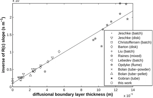
At this stage we have plotted in Fig. 4 the inverse of the slope of the experimental R(c) curves in Fig. 3 for each experiment against the DBL thickness δ. Despite the uncertainty in the determination of δ for each experimental device, the resulting curve is linear, as predicted by Eq. 2. So each experiment, according to its geometry and flowing configuration, probes a particular value of the boundary layer thickness 2. Thus the discrepancies between the dissolution rate constants in the literature stem mainly from the hydrodynamic differences between the experimental setups.
5
DISCUSSION
Now that a consistency has been recovered between the literature results, is it possible to get from these results a reliable pure surface raction rate constant, comparable to our holographic value? The extrapolation in Fig. 4 of a linear curve fitting all the literature data to δ = 0 gives scsat/(srks). To obtain ks from this value, the roughness factor ξ = sr/s is required, so we have to evaluate the mean reactive surface area srof the crushed samples used in the literature experiments.
Two topological classes of objects are known to have a strong influence on sr: etch pits and steps/kinks. For the first ones, we benefit from a recent thorough investigation by Atomic Force Spectroscopy of the
2We may just notice that the gap between Raines and Dewers (1997) measurements and the fitted law seems to
cleavage surface of gypsum during dissolution by Fan and Teng (2007). The main inference drawn from these experiments is the minor role of etch pits, remaining always shallow, in the process. The latter is governed by the fast dissolution of very unstable steps, whatever the solution undersaturation. This feature tends to enhance the similarity of gypsum with other minerals, where etch pits seem to contribute to dissolution not via the increase of reactive surface area but as source of monolayer steps inducing overall dissolution (Luttge et al., 2003; Gautier et al., 2001). For the second ones, we have too few informations at the moment about the behaviour of stepped and kinked faces of gypsum during dissolution to estimate their influence. So taking into account the AFM study we consider that the whole surface —for example measured by a BET adsorption experiment— is reactive, i.e., sr= sBET. Only one paper gives both its BET and geometric surface area values (Jeschke et al., 2001). As the roughness factor ξ = sr/s should be quite similar for all crushed gypsum samples, we have used the value of ξ = 1100/60 deduced from this work for all literature experiments. We have thereby computed ks = (∂R/∂c)δ=0csat/ξ and found ks = 7 × 10⁻⁵ mol m−2 s−1, which is the pure dissolution rate constant. This value agrees fairly well with our ks= (5 ± 2) × 10−5 mol m−2 s−1 holographic value. We can say that this coefficient had never been measured but can be deduced from the literature measurements a posteriori, and that it is much lower than all the rate constants proposed by the authors from their R(c) curves.
In a more graphical way, the resulting csat/(ξks) of our holographic value has been added in Fig. 4 at δ = 0. Remembering the experimental variability of ks, the dispersion of the literature values and the imprecision of the roughness factor ξ, the agreement between the value of ks extrapolated from the literature results and the value deduced from the holographic interferometry measurements is striking and validates both our analysis of the solution chemistry experiments and the accuracy of ks.
6
CONCLUSION
We have shown that despite apparent discrepancies, the correct consideration of the hydrodynamic condi-tions of the global dissolution experiments in literature brings a consistent view of the dissolution kinetics of gypsum in water and a pure surface reaction rate constant can be computed from all these measure-ments, much lower from what was expected. We have parallely measured by holographic interferometry this pure surface reaction coefficient in water at rest for various gypsum origins and surface morphologies. These two values agree well, thus validating a method able to provide benchmark values of dissolution rate constants of minerals.
This work has two methodological consequences. From a theoretical point of view, the holointerfero-metric tool may contribute to the evaluation of models. For instance, it permits to access directly to the prefactor K in the kinetic reaction law R = K exp [−∆G/(RT )] of the transition state theory or the disso-lution plateau A of the more elaborated model of Lasaga and Luttge (2001) of the dissodisso-lution of minerals, these both terms being merely equal to ks. From an experimental point of view, the underestimation of the transport contribution to the dissolution rate can help to explain the discrepancy between dissolution rates measured by local and global setups, for instance the very low value of the dissolution rate of calcite and dolomite in water measured by normal retreat of the surface via VSI, compared to values measured in bulk solution chemistry experiments (Arvidson et al., 2003; Luttge et al., 2003; Luttge, 2006).
Acknowledgements— We thank Elisabeth Charlaix and Jacques Bert for fruitful discussions, Nicolas Sanchez for experimental help, and Lucienne Jardin, Sylvain Meille and Pierre Monchoux for gypsum samples. This work was supported by Lafarge Centre de Recherche, R´egion Rhˆone-Alpes and CNES (french spatial agency).
References
Anderson, D. and Archer, D. (2002). Glacial-interglacial stability of ocean pH inferred from foraminifer dissolution rates. Nature, 416, 70.
Arvidson, R., Ertan, I., Amonette, J., and Luttge, A. (2003). Variation in calcite dissolution rates: A fundamental problem? Geochim. Cosmochim. Acta, 67, 1623.
Barton, A. and Wilde, N. (1971). Dissolution rates of polycristalline samples of gypsum and orthorhombic forms of calcium sulphate by a rotating disc method. Trans. Faraday Soc., 67, 3590.
Bolan, N., Syers, J., and Sumner, M. (1991). Dissolution of various sources of gypsum in aqueous solutions in soil. J. Sci. Food Agric., 57, 527.
Christoffersen, J. and Christoffersen, M. (1976). The kinetic of dissolution of calcium sulfate dihydrate in water. J. Crystal Growth, 35, 79.
Colombani, J. and Bert, J. (2007). Holographic interferometry study of the dissolution and diffusion of gypsum in water. Geochim. Cosmochim. Acta, 71, 1913.
Dreybrodt, W. and Gabrovsek, F. (2000). Comments on: Mixed transport / reaction control of gypsum dissolution kinetics in aqueous solutions and initiation of gypsum karst by Michael A. Raines and Thomas A. Dewers in Chemical Geology 140, 29-48, 1997. Chem. Geol., 168, 169.
Fan, C. and Teng, H. (2007). Surface behavior of gypsum during dissolution. Chem. Geol., 245, 242.
Gautier, J., Oelkers, E., and Schott, J. (2001). Are quartz dissolution rates proportional to B.E.T. surface areas? Geochim. Cosmochim. Acta, 65, 1059.
Gobran, G. and Miyamoto, S. (1985). Dissolution rate of gypsum in aqueous salt solutions. Soil Sci., 140, 89.
Hales, B. and Emerson, S. (1997). Evidence in support of first-order dissolution kinetics of calcite in seawater. Earth Planet. Sci. Lett., 148, 317.
Jeschke, A., Vosbeck, K., and Dreybrodt, W. (2001). Surface controlled dissolution rates of gypsum in aqueous solutions exhibit nonlinear dissolution kinetics. Geochim. Cosmochim. Acta, 65, 27.
Jordan, G., Pokrovsky, O., Guichet, X., and Schmahl, W. (2007). Organic and inorganic ligand effects on magnesite dissolution at 100 ◦c and ph=5 to 10. Chem. Geol., 242, 484.
Jousse, F., Jongen, T., and Agterof, W. (2005). A method to dynamically estimate the diffusion boundary layer from local velocity conditions in laminar flows. Int. J. Heat Mass Transfer , 48, 1563.
Kemper, W., Olsen, J., and DeMooy, C. (1975). Dissolution rate of gypsum in flowing water. Soil Sci. Soc. Am. Proc., 39, 458.
Keren, R. and O’Connor, G. (1982). Gypsum dissolution and sodic soil reclamation as affected by water flow velocity. Soil Sci. Soc. Am. J., 46, 26.
Lasaga, A. (1998). Kinetic theory in the earth sciences. Princeton University Press, Princeton.
Lasaga, A. and Luttge, A. (2001). Variation in crystal dissolution rate based on a dissolution stepwave model. Science, 291, 2400.
Lebedev, A. and Lekov, A. (1990). Dissolution kinetics of natural-gypsum in water at 5-25◦C. Geochem. Int., 27,
85.
Liu, S. and Nancollas, G. (1971). The kinetic of dissolution of calcium sulfate dihydrate. J. Inorg. Nucl. Chem., 33, 2311.
Luttge, A. (2006). Crystal dissolution kinetics and gibbs free energy. J. Electron Spectrosc. Rel. Phenom., 150, 248.
Luttge, A., Winkler, U., and Lasaga, A. (2003). Interferometric study of the dolomite dissolution: A new conceptual model for mineral dissolution. Geochim. Cosmochim. Acta, 67, 1099.
Figure 1: Scheme of the successive mechanisms occuring during the dissolution of a crystal grain in a bulk solution chemistry experiment.
Morse, J., Arvidson, R., and Luttge, A. (2007). Calcium carbonate formation and dissolution. Chem. Rev., 107, 342.
Opdyke, B., Gust, G., and Ledwell, J. (1987). Mass transfer from smooth alabaster surfaces in turbulent flows. Geophys. Res. Lett., 14, 1131.
Porter, E., Sanford, L., and Suttles, S. (2000). Gypsum dissolution is not a universal integrator of ’water motion’. Limnol. Oceanogr., 45, 145.
Raines, M. and Dewers, T. (1997). Mixed transport / reaction control of gypsum dissolution kinetics in aqueous solutions and initiation of gypsum karst. Chem. Geol., 140, 29.
Raju, K. and Atkinson, G. (1990). The thermodynamics of ”scale” mineral solubilities. 3. Calcium sulfate in aqueous NaCl. J. Chem. Eng. Data, 35, 361.
Rickard, D. and Sj¨oberg, E. (1983). Mixed kinetic control of calcite dissolution rates. Am. J. Sci., 283, 815.
Vinson, M. and Luttge, A. (2005). Multiple length-scale kinetics: an integrated study of calcite dissolution rates and strontium inhibition. Am. J. Sci., 305, 119.
Figure 2: Interferograms of the dissolution of a Mazan gypsum single crystal 20, 65, 105, 200 and 377 min. after the start of the experiment. The crystal is a thin grey line at the bottom of the optical cell.
0 2 4 6 8 10 12 14 16 0 1 2 3 4 5 6 7 8 x 10⁻⁴ concentration (mol l−1)
dissolution rate (mol m
−2 s −1 ) Jeschke (batch) Jeschke (disk) Christoffersen (batch) Barton (disk) Liu (batch) Raines (mixed) Lebedev (batch) Opdyke (flume) Bolan (tube−powder) Bolan (tube−pellet) Gobran (tube) c sat
Figure 3: Dissolution rates R of gypsum in water as a function of calcium concentration c for various setups. The R(c) curves are drawn from stirred batch experiments by Jeschke et al. (2001), Christoffersen and Christoffersen (1976), Liu and Nancollas (1971) and Lebedev and Lekov (1990), from rotating disk experiments by Jeschke et al. (2001) and Barton and Wilde (1971), from mixed flow/rotating disk reactor experiment by Raines and Dewers (1997), from shaken tube experiments by Bolan et al. (1991) (with powder or compressed powder pellets) and Gobran and Miyamoto (1985) and flume experiments by Opdyke et al. (1987). csat is the solubility of the dissolved calcium ions in water.
0 2 4 6 8 10 12 14 x 10−5 0 0.5 1 1.5 2 x 10⁵
diffusional boundary layer thickness (m)
inverse of R(c) slope (s m −1 ) Jeschke (batch) Jeschke (disk) Christoffersen (batch) Barton (disk) Liu (batch) Raines (mixed) Lebedev (batch) Opdyke (flume) Bolan (tube−powder) Bolan (tube−pellet) Gobran (tube) this work
Figure 4: Inverse of the R(c) slopes of Fig. 3 as a function of the diffusional boundary layer thickness δ for each setup.