HAL Id: hal-00317013
https://hal.archives-ouvertes.fr/hal-00317013
Submitted on 1 Jan 2002
HAL is a multi-disciplinary open access
archive for the deposit and dissemination of
sci-entific research documents, whether they are
pub-lished or not. The documents may come from
teaching and research institutions in France or
abroad, or from public or private research centers.
L’archive ouverte pluridisciplinaire HAL, est
destinée au dépôt et à la diffusion de documents
scientifiques de niveau recherche, publiés ou non,
émanant des établissements d’enseignement et de
recherche français ou étrangers, des laboratoires
publics ou privés.
To cite this version:
A. H. Manson, C. Meek, M. Hagan, J. Koshyk, S. Franke, et al.. Seasonal variations of the
semi-diurnal and semi-diurnal tides in the MLT: multi-year MF radar observations from 2?70° N, modelled tides
(GSWM, CMAM). Annales Geophysicae, European Geosciences Union, 2002, 20 (5), pp.661-677.
�hal-00317013�
Annales
Geophysicae
Seasonal variations of the semi-diurnal and diurnal tides in the
MLT: multi-year MF radar observations from 2–70
◦
N, modelled
tides (GSWM, CMAM)
A. H. Manson1, C. Meek1, M. Hagan2, J. Koshyk3, S. Franke4, D. Fritts5, C. Hall6, W. Hocking7, K. Igarashi8, J. MacDougall7, D. Riggin5, and R. Vincent9
1Institute of Space and Atmospheric Studies, University of Saskatchewan, Canada 2NCAR, Boulder NCAR, Boulder, USA
3Department of Physics, University of Toronto, Canada
4Space Science and Remote Sensing Laboratory, University of Illinois, USA
5Colorado Research Associates (a Division of Northwest Research Associates), Boulder, USA 6Auroral Observatory, University of Tromsø, Norway
7Department of Physics and Astronomy, University of Western Ontario, Canada 8Communications Research Laboratory, Tokyo, Japan
9Department of Physics and Mathematical Physics, University of Adelaide, Australia
Received: 20 July 2001 – Revised: 14 December 2001 – Accepted: 18 December 2001
Abstract. In an earlier paper (Manson et al., 1999a) tidal data (1990–1997) from six Medium Frequency Radars (MFR) were compared with the Global Scale Wave Model (GSWM, original 1995 version). The radars are located between the equator and high northern latitudes: Christ-mas Island (2◦N), Hawaii (22◦N), Urbana (40◦N), London (43◦N), Saskatoon (52◦N) and Tromsø (70◦N). Common harmonic analysis was applied, to ensure consistency of am-plitudes and phases in the 75–95 km height range. For the diurnal tide, seasonal agreements between observations and model were excellent while for the semi-diurnal tide the sea-sonal transitions between clear solstitial states were less well captured by the model.
Here the data set is increased by the addition of two lo-cations in the Pacific-North American sector: Yamagawa 31◦N, and Wakkanai 45◦N. The GSWM model has
under-gone two additional developments (1998, 2000) to include an improved gravity wave (GW) stress parameterization, back-ground winds from UARS systems and monthly tidal forc-ing for better characterization of seasonal change. The other model, the Canadian Middle Atmosphere Model (CMAM) which is a General Circulation Model, provides internally generated forcing (due to ozone and water vapour) for the tides.
The two GSWM versions show distinct differences, with the 2000 version being either closer to, or further away from, the observations than the original 1995 version. CMAM provides results dependent upon the GW parameterization
Correspondence to: A. H. Manson
(manson@dansas.usask.ca)
scheme inserted, but one of the schemes provides very useful tides, especially for the semi-diurnal component.
Key words. Meteorology and atmospheric dynamics
(mid-dle atmosphere dynamics; waves and tides)
1 Introduction
The study of atmospheric tides in the middle atmosphere (MA) is important for a variety of reasons. Their ampli-tudes are generally the largest of all the atmospheric oscil-lations (Gravity, Planetary, Tidal waves), e.g. Manson and Meek (1986), and although seasonal variations are usually quite strong at all latitudes they are still the most regular and persistent oscillations. Tides are known to have a significant impact upon the momentum balance in the lower thermo-sphere (>∼ 90 km), especially at lower latitudes (Forbes et al., 1993; Miyahara et al., 1993), and upon the distribution of atmospheric constituents (Shepherd et al., 1998; Ward, 1998). They also modulate the fluxes of propagating GW (Manson et al., 1998).
Tidal structures in the MA are extremely complex, so that successful modelling requires the understanding of a wide range of atmospheric phenomena, including radia-tional, chemical and dynamical. These include the distri-bution of ozone and water vapour in height, season and planetary location; the background winds and mean tem-peratures; molecular and eddy diffusivity; and gravity wave stress and Newtonian cooling effects. In mechanistic models like GSWM such processes are parameterized in the model.
characterizations, and also the advantages of monthly reso-lution. Our earlier paper (hereafter Paper 1, Manson et al., 1999a) compared GSWM with a seven year (1990–1997) MFR data set; here that set is supplemented with observa-tions (1996) from Wakkanai (45◦N) and Yamagawa (31◦N).
The assessment of tides within a Global Circulation Model (GCM), in this case CMAM, is also challenging to the mod-elling enterprise. Here one is testing in a very comprehen-sive manner the internal consistency and comprehencomprehen-sive na-ture of the model. Elsewhere (Manson et al., 2001) we have analysed the seasonal outputs from CMAM for three GW parameterization experiments to obtain GW intensities, tidal amplitudes, and phases for the solar semi-diurnal and diur-nal tides for 7 MFR locations. These were compared with the observed GW characteristics (Manson et al., 1999b) and tidal characteristics (in this case the tidal data were mainly from the 2 years of MFR observations in 1993/1994). Briefly, the modelled tides depended strongly upon parameteriza-tion, and the MFR comparisons led to a preference for the Medvedev and Klaassen (2000) scheme. Amplitudes from CMAM were quite similar to those observed for the semi-diurnal tide; but modelled semi-diurnal tides were much larger at low latitudes (0–22◦N), in the equinoxes, and at higher latitudes, in summer, than observed. The semi-diurnal tidal phases were often in very good agreement for CMAM and MFR with longer/shorter vertical wavelengths generally at lower/higher latitudes; while for the diurnal tide, although the phase gradients (height, latitude) were quite similar for the MFR and CMAM at lower latitudes, consistent with the short wavelength S (1, 1) mode, they differed significantly at higher latitudes. It will be interesting here to compare CMAM tides with not only a larger MFR data set (7 years rather than 2) but also with GSWM 2000 (Sect. 6).
2 The models: GSWM, GSWM2000; CMAM
GSWM is a two-dimensional linearized model that solves the Navier-Stokes equations for tidal and planetary wave perturbations as a function of latitude and altitude, for a specific wave periodicty and zonal wave number:
http://www.hao.ucar.edu/public/research/tiso/gswm/gswm.html. Essential references for the GSWM include the following: Hagan et al., 1993, 1995; Manson et al., 1999a; Hagan et al., 1999. The last reference and the web-site describes the 1998 version of GSWM which is the foundation for GSWM2000.
invoked in both GSWM and GSWM1998. Otherwise, the assumptions invoked in GSWM2000 are identical to those that characterized GSWM1998 (Hagan et al., 1999) with the single exception of the ozone model used to parameterize strato-mesopheric migrating tidal forcing. CIRA ozone cli-matologies (Keating et al., 1990) were used in both GSWM and GSWM2000, since Hagan et al. (1999) demonstrated negligible impact when UARS measurements replaced the CIRA model in GSWM1998. Preliminary evaluations of the GSWM2000 may be seen in Hagan et al. (2001) and Pancheva et al. (2001).
The following brief description gives the highlights of GSWM2000 in so far as it differs from the other model used, GSWM (originated in 1995). Both models use mean temperatures and densities from Hedin (1991), the same winds below 12 km (Groves, 1985, 1987) and tropospheric migrating tidal forcing (Groves, 1982). However while GSWM used middle atmosphere winds from Groves (1985, 1987) and an empirical wind-model due to Portnyagin and Solov’era (1992a, b), the latest GSWM versions (1998, 2000) use UARS-HRDI (High Resolution Doppler Interfer-ometer) winds (Hagan et al., 1999; after Burrage et al., 1996). This is a significant change, as shown by Hagan et al. (1999). For ozone tidal forcing the CIRA distributions (Keating et al., 1990) are used for 1995 and 2000 versions. The models also use the same molecular and eddy diffusivity schemes and pa-rameterizations for ion drag and Newtonian cooling effects. Gravity wave stress in the form of linear (Rayleigh) friction on the diurnal tide now varies monthly, with GSWM2000 equinox values an order of magnitude smaller than for the solstices (Hagan et al., 1999). The latter are very close to the constant values of stress used in GSWM. This change was initiated to provide diurnal tidal amplitudes at low latitudes which matched the large equinoctial analysed tides from the HRDI data (Burrage et al., 1995). The monthly diurnal and semi-diurnal data from GSWM2000 are obtained by using either input background data, which are inherently monthly, or by interpolation of the background data. Factors not in-cluded in either model include these: thermospheric in-site forcing and latent heat release due to convective activity in the troposphere. In all figures the GSWM data are shown for the middle month of the season only, as this month will be more representative of average conditions for the season and these were used in the model as background conditions.
The CMAM is a 3D spectral GCM extending from the ground to a height of approximately 100 km (Beagley et al.,
1997). The prognostic fields are expanded in a series of spherical harmonic functions with triangular truncation at to-tal wavenumber n = 47 (T47) corresponding to a horizonto-tal grid spacing of about 400 km. The model contains 50 lev-els in the vertical with a resolution of approximately 3 km above the tropopause. Realistic surface topography, plane-tary boundary-layer effects, a full hydrological cycle, a pa-rameterization of moist convective adjustment including the release of latent heat and comprehensive shortwave (solar) and long-wave (terrestrial) radiation schemes are all included in the model. The radiative effects of clouds are included also. Both diurnal and semi-diurnal global tides are forced by CMAM. The reader is referred to (Beagley et al., 1997) for further details.
The finite resolution of CMAM and other GCMs makes it impossible to represent explicitly the effects of GW with spatial scales smaller than the model grid spacing. (Note that resolved GW, with scales larger than the model grid spacing, are routinely excited in the model by a variety of sources including shear instabilities and flow over topogra-phy). In order to represent the effects of unresolved (subgrid-scale) GWs on the resolved flow, GW drag parameterization schemes are often invoked. The parameterization of drag due to the breaking of waves excited by subgrid-scale topog-raphy is described in McFarlane (1987) and this scheme is included in all simulations presented here. The effects of GW that may arise from unresolved non-orographic sources such as moist convection and dynamical shear instabilities in, for example, frontal zones, are represented in the data shown here by a scheme due to Medvedev and Klaassen (1995). A simple Rayleigh-drag “sponge” layer is also em-ployed above the 0.01 mb level (∼ 80 km) in order to prevent the reflection of upward propagating waves at the model up-per boundary. Although not particularly realistic, the sponge layer can be regarded as a crude representation of GW drag in the mesopause region above 80 km. In fact CMAM data up to 88 km are used, as the tidal phases continue to be smoothly and realistically varying from 80–88 km (Manson et al., 2001).
CMAM data used in this paper consist of horizontal winds sampled every 20 min. Data are archived on 15 pressure lev-els between 60 and 90 km, for a nominal vertical resolution of approximately 3 km. Results for the months of January, April, July, and October only are highlighted here; and these involve 30 day sequences of continuous data.
3 The MFR systems and data
The initial analysis applied to the radar data is the full-correlation analysis (FCA) for spatial antenna systems. The variant developed by Meek (1980) is used for the more northern stations (Tromsø 70◦N, Saskatoon 52◦N, London 43◦N, Urbana 40◦N) partly due to its usefulness in deal-ing with correlograms that are noisier or multi-peaked; while a more classical Brigg’s method is used at the other sta-tions (Isler and Fritts, 1996): Wakkanai 45◦N, Yamagawa
31◦N, Hawaii 22◦N, Christmas Island 2◦N. Comparisons
have shown no significant differences exist between these methods (Thayaparan et al., 1995). The radars provide sam-ples of wind every 2 or 3 km (ca. 70–100 km) and 2 or 5 min on a continuous basis.
It should be noted that very thorough comparisons ex-ist between winds and tides measured by the MFR and other ground based systems: MWR (Meteor Wind Radar) and MFR radars at 40◦N (Hocking and Thayaparan, 1997); MFR and Fabry-Perot Interferometers (“green line” and hy-droxyl) at 52◦N (Manson et al., 1996; Meek et al., 1997); and MFR, EISCAT (European Incoherent Scatter) and VHF radars (Manson et al., 1992) at 70◦N. In all of these studies the phases of the tides or directions of the winds have been quite satisfactorily consistent once the system-differences were considered; e.g. differences in data-yield with respect to local time. The amplitudes of tides or wind speeds were in good agreement (typically within 10%) in some cases, e.g. the optical and radar comparisons, but not in others. In par-ticular, at 70◦N, the tidal amplitudes and wind speeds from the MFR were 0.65 of those from the VHF radar and rockets (80–90 km). This result is similar to the differences found be-tween HRDI-UARS and MFR systems; e.g. at Saskatoon the MFR speeds are 0.70–0.8 of those from HRDI (Meek et al., 1997). Also, a recent MFR-MWR comparison at Saskatoon showed ratios of 0.85 (Meek and Manson, Private commu-nication, 2000). As the reason for these ratios is not fully understood at present, we will simply bear this in mind when later comparisons are made in this paper.
A common analysis has been used at each radar location to obtain the amplitudes and phases of the monthly diurnal and semi-diurnal oscillations in the wind field. For each month of available years (1989–1996), an harmonic analysis was applied to the entire 28–31 day time series of hourly values (zonal, E–W; meridional, N–S), for the 12 and 24 h oscilla-tions (amplitude and phase), to better compare with a mod-elled month. We required that, for each fit, there were data for 16 h or more of the 24 possible for each height over the month; also weighted the hourly means in the fit according to the number of values therein. Values of the monthly am-plitudes and phases from the completed fits were retained when the standard deviations (sd) of the phases were less than 2.5 and 5 h, respectively; these were obtained from the variances of the least-squares-fits (harmonic analysis). The restriction on the sd was used as a measure of the quality of the fit; this particular choice eliminates noise and provides smoothly varying phases profiles. The minimum height pos-sible to meet these criteria then varied from 70–85 km while the maximum height was restricted to values below the lo-cal estimates or lo-calculations of total reflection of the radar pulse. This latter is generally between 90–100 km. A similar analysis was applied to wind time-sequences (Sect. 2) from CMAM for Sect. 6.
The intention of the data presentations is to focus upon the main features of agreement or disagreement between the ob-servations and the models and also to show the global struc-tures of the tides. These comparisons serve as a further
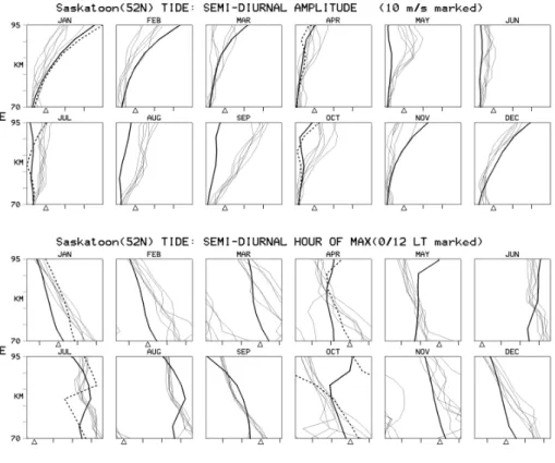
eval-Fig. 1. Profiles of the Semi-Diurnal (12 h) Tide amplitudes and phases for the zonal (E) component at Saskatoon. The thin lines are for the 6 years of MFR data, the dashed lines for GSWM (original 1995) and the thick lines for GSWM2000. The triangles on the am-plitude plots refer to the 10 m/s val-ues. For the phase plots the total phase displayed is 12 h; the triangles are at 00:00 and 12:00 LT and their positions are chosen to minimize the number of phase discontinuities (“wrap-around”).
Fig. 2. Profiles as for Fig. 1, but for
Hawaii.
uation of GSWM2000. The figures have been designed to provide easy appreciation of these features. In Sects. 4 and 5 we shall show some monthly MFR profiles for high and low latitudes where the semi-diurnal and diurnal tides, respec-tively, are dominant and add to those the GSWM profiles. Then, for the 90 km altitude, latitudinal plots by month are
shown for both tides, again with the two models. Finally in those sections we shall show new plots of amplitudes and phase contours as functions of height and latitude, for the middle month of each season. Each data presentation for-mat has a particular advantage and together they provide a very comprehensive test of agreements between models and
the MFR observations. The last named are valuable in that they show global structure particularly well; it will be seen that differences between GSWM and GSWM2000 are well distinguished in the phase plots. Finally, in Sect. 6, we will show profiles for all stations in the middle months of each season and include the two GSWM and CMAM. As men-tioned, CMAM tides are investigated elsewhere (Manson et al., 2001) but this format and the GSWM comparison are new.
4 Semi-diurnal tides
4.1 Monthly profiles; Saskatoon 52◦N, Hawaii 22◦N
We have chosen to use these two stations where the low and high latitude characteristics of the tidal winds are well dis-played. The semi-diurnal (12 h) tide is significantly larger than the diurnal (24 h) tide at Saskatoon while the diurnal tide is the larger at Hawaii. The tide is generally circular at both locations, with 3 h differences between NS and EW compo-nents (“quadrature”), so that only one component (EW in the figure) will be shown here. Those readers interested in the larger MFR data set should acquire the full ISAS Re-port (Manson et al., 1999c). Times shown in the phase-plots are for maximum perturbations in the North and East direc-tions. The individual years of MFR data are not marked to remove confusing detail in Figs. 1 and 2, and the interan-nual variations will be discussed elsewhere. Generally these variations are modest, indicating that modelling using mean background conditions should approach the median profiles of the up to 7 years of data. The plotting algorithm selects the smallest phase difference between any two heights to min-imize ’wrap-around’ effects and also the triangle marking 01:00 and 12:00 LT is placed to minimize these effects.
Considering first Fig. 1 for 52◦N, the amplitude ob-servations are smaller than the GSWM models in winter months but otherwise are significantly larger, especially in the spring and autumn. These features were discussed in Paper 1 (Sect. 5) where it was noted that semi-diurnal tro-pospheric latent-heating effects approach 10 m/s in the up-per MA (Forbes et al., 1999). Such additional tidal compo-nents, while helpful, would not be likely to account for the large equinoctial differences. Otherwise, the ∼ 20% possible speed bias (MFR small), noted in Sect. 3 for the Saskatoon MFR, would help the winter comparison and worsen that for the rest of the year. The differences between GSWM and GSWM2000 are usually small. Note that the GSWM pro-files for each month of each season are constant (and in the figure they are only shown for the middle month of the sea-son), whereas GSWM2000 has unique monthly values. The latter’s winter reductions in amplitude are helpful in the com-parison.
Moving to the phases, the observations show stable sol-stitial structures with larger phase slopes (described for con-venience as shorter wavelengths) in winter and altitudinally varying slopes in summer;these are strikingly consistent over
the two seasons and inter-annually. The phase values for GSWM and GSWM2000 are usually similar to observations in the middle of the sampled heights although the phase-slopes are not very similar to the MFR, e.g. 80 km vs. 40 km in winter. It is not clear which model is better overall. How-ever, the summer phase discontinuity of GSWM, which was associated with unobserved short wavelengths at high lati-tudes, has largely gone in GSWM2000. The observed tran-sitions during the equinoxes are substantial and, although the inter-annual variability is larger in those months, clearly defined monthly phase values and slopes are still evident. Again, while the modelled phases are usually overlapping observations at some heights the phase slopes usually dif-fer. Overall the phases for GSWM2000 are, as a percentage of the 12 frames in Fig. 1, marginally better than the 1995 GSWM version.
Comments on the 22◦N profiles in Fig. 2 will be brief now
that the pattern of commentary has been set. Observed ampli-tudes are generally larger than the models, especially below 90 km; the decreases above 90 km may be the MFR speed-bias effect. The GSWM2000 values are generally similar to GSWM but the increases in the autumn season come closer to matching the MFR observations. Considering phases, the observed profiles are quite consistent for most months and demonstrate small phase-slopes (wavelengths of about 100 km). The modelled phases for both GSWM versions of-ten have similar slopes to those observed although the two models differ in the autumn. Overall, apart from the striking summer agreements in June and July, the observed and mod-elled phase values differ significantly (often 6 h or more). 4.2 Latitudinal plots at 90 km
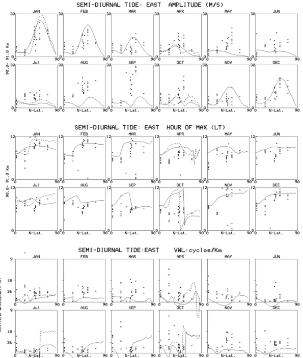
These plots allow multi-latitude comparison of amplitude and phase, again for the EW component (Fig. 3); the NS plots (not shown) are very similar and add little to the study. The phase structures can be inferred to a degree from the in-verse of the phase-slope, which we abbreviate as an effective wavelength. Although the slopes are calculated over a 6 km interval near 87 km, the wavelength values usually agree with the characteristics slopes over the 75–95 km height range ev-ident in Figs. 1 and 2. This was well established in Paper 1.
The amplitude plots of Fig. 3 show that the earlier pro-files for 22◦ and 52◦N were thoroughly representative of the global pictures. Except for the 5 winter-like months (November to March) the middle to high latitude obser-vations are larger than the modelled values with low lati-tude observations also being larger in summer and autumn. Note that there are two additional MFR locations, at Yama-gawa (35◦N) and Wakkanai (45◦N). Their data generally fit smoothly into the existing data. The two sets of GSWM am-plitudes are quite similar, although in winter the GSWM2000 values are smaller and closer to the observations. Again the phases mirror Figs. 1 and 2, with values at higher lat-itudes being within 2–3 h of the models but differing more frequently at lower latitudes. Generally the differences are large (about 6 h) in September and October when the
ampli-Fig. 3. Latitudinal plots for the zonal (East) component of the Semi-Diurnal (12 h) Tide near 90 km. The dots are for all of the available years
at the MFR locations; these now include Christmas Island 2◦N, Hawaii 22◦N, Yamagawa 31◦N, Urbana 40◦N, London 43◦N, Wakkanai 45◦N, Saskatoon 52◦N, Tromsø 70◦N. As before, the solid lines are for GSWM and the dashed for GSWM2000. The phase-gradients, interpreted here as vertical wavelengths, are over 6 km centred on 87 km.
tudes also differ substantially; this suggests substantial dif-ferences in the tidal Hough-mode composition in this sea-son. Note that, while the phase-agreements near 90 km may be relatively good, the phase-slopes may differ and thus give poorer phase-agreement at other heights i.e. Fig. 1.
The phase-slopes, converted to an equivalent wavelength, also emphasize the generality of the earlier profiles. Above 22◦N, observed winter wavelengths are smaller (about half, 40 vs. 80 km) than modelled whilst, in summer, observed values are long or irregular (the cross indicates a negative slope) which is in good agreement with the models. (In the
summer case the combination of small phase gradients and random fluctuations (noise) will have led to some of these negative values; others will be legitimate and relate to su-perposition of tidal-modes.) This agreement is especially true for GSWM2000 at high latitudes where the problem-atic short values (18 km) of the original GSWM version have been avoided. The modelled values in spring are too large and, in autumn, show more latitudinal variability than is observed. Apart from the important summer improvement, GSWM2000 is not significantly different from the original version at latitudes beyond 22◦N. At the lowest latitudes, the
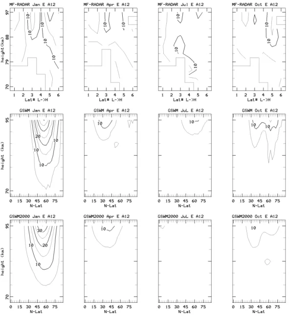
Fig. 4. Amplitude (A12) contour plots for the zonal component of the 12 h Tide. Plots are shown for the MFR systems (Latitude numbers
1–6; Christmas Island, Hawaii, Urbana, London, Saskatoon and Tromsø), the GSWM, and the GSWM2000. The numbers on the lines are in m/s; +ve meaning toward the east.
Christmas Island (2◦N) observations are often similar to the models and, at Hawaii (22◦N), observed and modelled val-ues are often large or negative.
4.3 Contour plots: height versus latitude
The new EW contour plots (Figs. 4 and 5) very nicely sum-marize the above comparisons (The NS are very similar). The model values are plotted versus latitude; the radar loca-tions (shown as numbers 1–6) are at Christmas Island (2◦N), Hawaii (22◦N), Urbana (40◦N), London (43◦N), Saskatoon (52◦N) and Tromsø (70◦N). These are reasonably evenly spaced, except for the two sites near 40◦N, and for these small-scale contour plots model-radar comparisons are quite straight-forward. Although absolute comparisons of values
are less obvious, the tidal structures are ideally displayed (Here the new 31◦and 45◦N data are not incorporated as they are from one year only, while 7 years are used for the other MFR systems to form means). The amplitudes are arithmetic means of the annual-monthly values. In Fig. 4 the modelled higher latitude large-amplitude cell of winter is very clear; and, as expected from Fig. 3, the observed January month also shows a maximum, albeit somewhat weaker. However, it is clear from the annual profiles and 90 km values (Figs. 1 and 3) that values approaching those of the model do oc-cur in some years. Given that the phase-slopes also differ (Fig. 5) it is clear that a particular tidal Hough-mode in the model has been amplified. The observed phase structures for the four months generally vary quite smoothly although, in the equinoxes, there are a few localized regions with strong
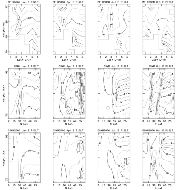
Fig. 5. Phase (P12) contour plots for the 12 Tide. Otherwise, as in Fig. 4. The numbers on the lines are for the time of maximum eastward
wind (+ve).
shears which are due to the variability of the season, lo-cal tidal structures and data points of greater uncertainty. Nevertheless, wavelengths are consistently longer/shorter at low/high latitudes, except that summer has shorter/longer values at lower/upper heights at mid-latitudes (Fig. 1). The models also generally demonstrate shorter wavelengths at higher latitudes. Without going into detail, because the com-ments of Sects. 4.1 and 4.2 are generally appropriate here, the GSWM2000 structures are clearly preferable to the GSWM, especially in spring and summer. However, the vertical phase gradients in the two GSWM versions differ clearly from the observations.
In conclusion, while GSWM2000 is a modest improve-ment for the semi-diurnal tide, significant differences still remain in modelled amplitudes and overall phase-structures
with the Pacific-North American sector MFRs. Neither GSWM may be said to model the semi-diurnal tide well. As noted earlier, additional tidal components forced by tro-pospheric latent heat release may improve the GSWM ca-pabilities. Also, GSWM may be missing a fundamental migrating tidal component. It should also be remembered that the observed oscillations will potentially contain non-solar-migrating tidal components. Measurements of longi-tudinal variations in tidal characteristics are thus very valu-able. The most useful assessment is by Jacobi et al. (1999), who showed that, while the semi-diurnal tidal phase struc-tures near 52◦N were very similar between 4◦W–49◦E and 107◦W, the amplitudes in winter and autumn were doubled at 49◦E and 107◦W compared with Western Europe and
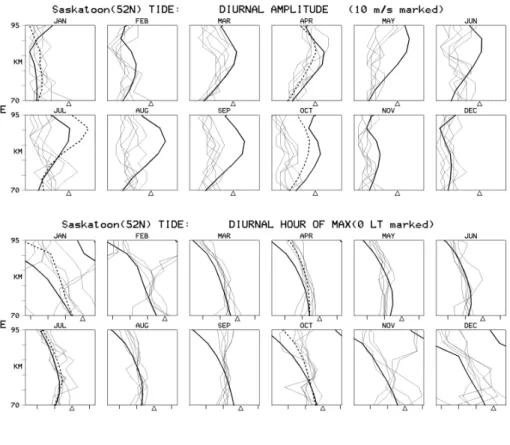
Fig. 6. Profiles of the Diurnal (24 h)
Tide amplitudes and phases for the zonal (E) component at Saskatoon. The thin lines are for the 6 years of MFR data, the dashed lines for GSWM (original 1995) and the thick lines for GSWM2000. The triangles on the am-plitude plots refer to the 10 m/s val-ues. For the phase plots, the total phase displayed is 24 h; the triangles are at 00:00 LT and their positions are chosen to minimize the number of phase dis-continuities (“wrap-around”).
Fig. 7. Profiles as for Fig. 6, but for
Hawaii.
longitudinally-varying data set. Similar longitudinal varia-tions in amplitude where shown in the summer months of 1999 by Pancheva et al. (2001).
We make a brief comment on the comparisons between radar and GSWM2000 tidal winds by Pancheva et al. (2001).
These were for a 3-month summer (June–August) campaign in 1999 with 15 northern hemisphere radars. Results were restricted to heights near 90 km. Thus, comparative figures were restricted to the style of Figs. 3 and 8, with latitudi-nal plots of amplitudes, phases and phase gradients (inferred
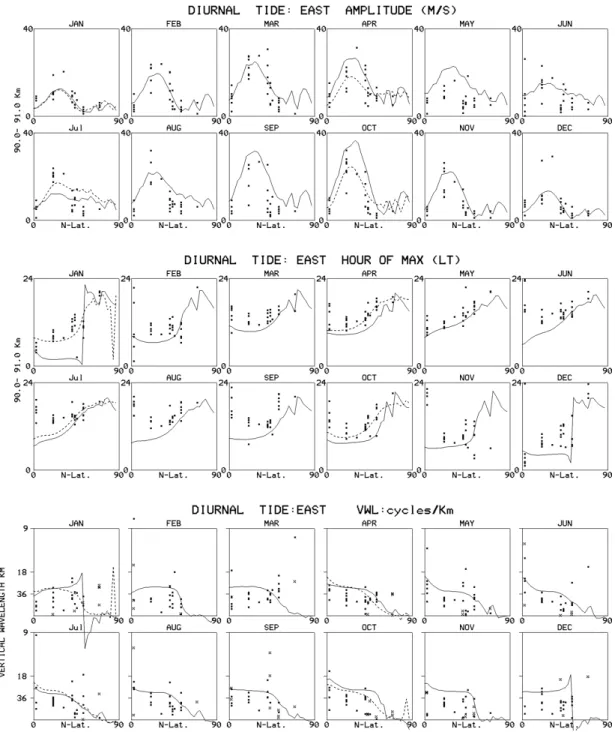
Fig. 8. Latitudinal plots for the Diurnal Tide (24 h) near 90 km. Otherwise as for Fig. 3.
vertical wavelengths). Where possible, latitudinal averages of radar data were used but only latitudes near 50◦N al-lowed for significant smoothing of any longitudinal variabil-ity. The phase and amplitude height structures revealed by our Figs. 1, 2, 4 and 5 (and our subsequent figures for the diurnal tide) were not available from their observations, nor was the GSWM2000 assessed in that fashion, e.g. our Figs. 4 and 5. However, the results shown by Pancheva et al. (2001) are very similar to those shown in Fig. 3 and discussed above, consistent with several of the radars contributing data to both studies and the modest inter-annual variability shown in our figures.
5 Diurnal tides
5.1 Monthly profiles; Saskatoon 52◦N, Hawaii 22◦N
We shall follow the same pattern of presentation as in Sect. 4. The models and observations for Saskatoon show similar am-plitudes and profile shapes in winter and spring (Fig. 6), while in summer-like months and autumn the models are larger. The equinoctial values for GSWM2000 are larger than the original GSWM, due to the new GW stress, but are smaller in summer months. These mid-latitude differences between model and MFR are probably real, as the possible
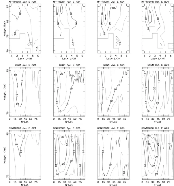
Fig. 9. Amplitude (A24) contour plots for the zonal component of the 24 h Tide. Otherwise as for Fig. 4.
MFR speed bias factor (reductions) is only circa 20% below 90 km. Also, the observed phase structures are remarkably consistent inter-annually and by month, although the winter months are more variable, probably due to planetary waves and stratospheric warmings (STRATWARMS). As discussed in Paper 1, the phase-agreement with GSWM is remarkably good in all months, and represents the first successful mod-elling of non-winter months at mid-latitudes. As expected GSWM2000 is consistent with GSWM, but it does show a consistent phase-offset.
Figure 7 shows the data from Hawaii. The modelled and observed amplitudes are quite similar in winter and summer but, in the equinoxes, the modelled values, espe-cially GSWM2000, lie just beyond the observed ranges of values. The new model is again larger than the original GSWM. However allowing for a possible 20% MFR speed
bias, which generally increases with height, the agreement would be satisfactory. The observed phases are consistent by month and year and the agreement with modelled values, possibly between 85 and 90 km, is generally good (phase dif-ferences are generally less than 3 h). However, the observed wavelengths are generally larger than modelled, especially in winter. And again, usually the GSWM2000 is further away from the data than is GSWM.
The EW amplitude plots of Figs. 6 and 7 were quite rep-resentative of the entire low and mid-to high latitude char-acteristics (Fig. 8). The new data for 31◦N and 45◦N are generally consistent with neighbouring latitudes. Apart from the previously mentioned smaller values observed in summer and autumn at higher latitudes, the agreement with the mod-els is very good. However, the otherwise desirable increase in equinoctial amplitudes in GSWM2000 moves the curves
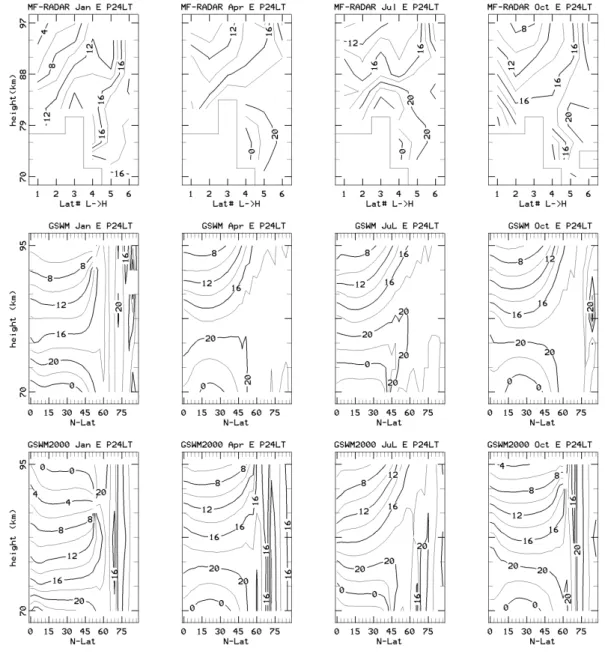
Fig. 10. Phase (P24) contour plots for the 24 h Tide. Otherwise as for Fig. 9.
away from the data, a trend probably compensated for by the probable MFR’s speed bias. The NS plots (not shown) are generally similar, except in the equinox where low lati-tude GSWM2000 peak values are always larger (by a factor of two) than observed. Considering the phases, the agree-ment of observations with GSWM is excellent at 90 km (see Paper 1 for detailed discussions) but with the tendency for the low-latitude model values to lead the observations (also Fig. 7). Also, the new model’s phases are generally in poorer agreement by 2–3 h due to a consistent offset. Consider-ing the complexity of mid-latitude diurnal tides, this gener-ally close agreement with the original GSWM is remarkable while that with the new model is not representative of the data despite new and desirable features in the new version (Sect. 2).
Finally, considering the corresponding wavelengths, Fig. 8
provides generalization of the profile results of Figs. 6 and 7. Thus at mid-latitudes throughout much of the year, the mod-elled wavelengths are smaller than observed, especially for GSWM2000; and at low latitudes, and especially for Hawaii, the modelled values are also smaller. This latter effect was noted earlier in comparisons between observed HRDI and MFR winds (Burrage et al., 1996), and has not been resolved. Differences between the two models are small, with GSWM being closer to observations in 6 months of the year. 5.2 Contour plots: height versus latitude
The amplitude (EW) contours (Fig. 9) show the modelled low-latitude equinoctial maxima very clearly; although the observations match GSWM quite well they are smaller than the new model version. It is particularly desirable that low-latitude radar observations be extended down to 70 km to
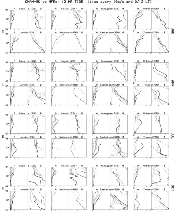
Fig. 11. Comparisons between profiles for the Semi-Diurnal (12 h) Tide amplitudes and phases from the 8 MFR systems (thin lines), the
Canadian GCM (CMAM) with the thick lines and the GSWM (thick dashed lines). The monthly means for winter, spring, summer and autumn (central) months are shown.
check the very large modelled values there. As mentioned in Sect. 5.2, the modest MFR speed-bias would minimize these differences. In other seasons, modelled amplitudes are rather similar to observations although, as noted in Figs. 6 and 8, the modelled values at middle latitudes are usually larger (10 vs. 5 m/s) than observed even if an MFR bias cor-rection is applied. Observed phase structures (Fig. 10) vary quite smoothly with height and latitude, providing vertical phase-slopes consistent with shorter wavelengths (ca. 35– 40 km) at low latitudes and longer (evanescent to 50km) at
high latitudes (> 50◦N). The shortest high-latitude values
occur in winter. The two models show this transition between dominant tidal structures very clearly. However GSWM is clearly closer to observations, since for the 2000 version un-observed shorter structures have spread and are dominant at Saskatoon (52◦N) in winter, spring and autumn (as in Fig. 6). It is probable that this extension to higher latitudes is also as-sociated with their larger amplitudes, as mentioned above. In this case the NS component of GSWM2000 (not shown) is also interesting as the short wavelength structures do not
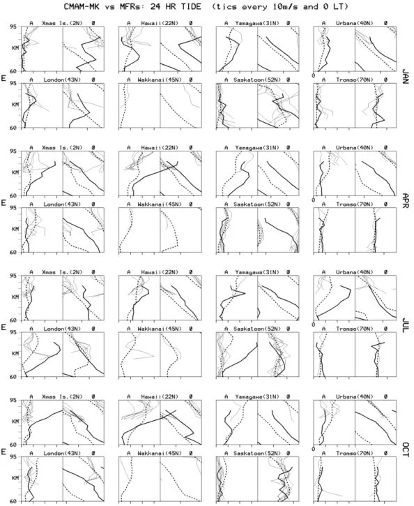
Fig. 12. Comparisons between the Diurnal (24 h) Tide profiles for the MFR and GSWM. Otherwise as for Fig. 11.
reach as far north (∼ 5◦difference). This difference between the two components is indeed weakly evident at Saskatoon in the original GSWM version and was discussed in Paper 1. Overall then, and as discussed fully in Paper 1, the original GSWM agrees very well with observations.
In summary, the new model is not an improvement over GSWM, especially with regard to phase structures. As with the semi-diurnal tide, the incorporation of latent heat ef-fects into GSWM versions would provide tidal modes which could, through superposition, modify amplitudes and phases. Again, longitudinal variability of the tides could be respon-sible for some of the differences between the new model
and the observations, rather than the simpler conclusion that GSWM is the better model. Pancheva et al. (2001) show very modest observed summer phase-changes with longitude (near 90 km) and larger amplitude changes (a factor of 2); these comparisons were for a latitude range of 43–56◦N, which is broad enough to partly obscure the real variability. However, the amplitudes for the North American-Pacific sec-tor (near 50◦N) were larger than for Europe in the summer months which does not help the comparisons in Figs. 8 and 9. The different zonal winds in the two GSWM versions will also be a factor in the different tidal-winds which have been produced. A final thought, which leads directly into Sect. 6,
Table 1. Percentage of “better” matches
GSWM CMAM Models similar 12 h SD tide Amplitude 4% 80% 16% Phase 11% 27% 62% 24 h D tide Amplitude 56% 12% 32% Phase 73% - 27%
NB: Only 3% of the cases had neither model close to the observa-tions. (The remaining cases represent the 100% above.)
is that GW stress or drag and the eddy diffusion effects upon momentum and heat fluxes are not as realistic as desirable. In Manson et al. (2001) the differing effects of two parameteri-zation schemes (Medvedev and Klaassen, 1995; Hines, 1997; Medvedev and Klaassen, 2000, where there are comparative discussions) were shown to have profound implications for hemispheric CMAM amplitude and phase structures. Below we discuss results from the former (MK) scheme in a CMAM experiment.
As for the semi-diurnal tide, we comment briefly on the summer (June–August, 1999) comparisons between radar and GSWM2000 tidal winds by Pancheva et al. (2001), for heights near 90 km. In figures similar to our Fig. 8, they also found very good agreements for amplitudes and phases.
6 Semi-diurnal and diurnal tides from CMAM
The time-sequences for the MFR locations were obtained from the CMAM-MK experiment and analysed in identical fashion to the radar data. We have chosen a profile format so that variations with height at the eight latitudinally-varying locations may be studied for amplitude and phase. Contour plots are shown elsewhere (Manson et al., 2001). Inspection of Fig. 11 for the semi-diurnal tide, where thin lines are for the MFRs and thick lines are for the CMAM, shows gener-ally very good agreement at all latitudes and most seasons but with apparently excessive summer CMAM amplitudes at middle to high latitudes and phase disagreements at 31◦N in winter and spring. The GSWM (thick dashed-line) has been added for comparative purposes and is clearly less similar to the MFR than is the CMAM. We chose GSWM as the semi-diurnal tides are similar in both versions but the semi-diurnal tides are closer to observations in that version. The percentages of best-matches are shown in Table 1. The model in “better” agreement with observations is selected at each location and season but, if both models are close to the observations, the “similar” choice is made. Usually one or other model-profile passes through the data at several heights. In only two or three cases out of 60 does neither model satisfy these condi-tions for “similar” or “better”. The CMAM amplitudes are “better” for 80% of the choices, while for phases CMAM is “better” for 27%, with CMAM and GSWM being “similar”
for 62% of choices. We recall that the GSWM (Sect. 4) suf-fered from consistently low amplitudes. When comparisons of CMAM and GSWM2000 with the MFR are made the per-centages are very similar but with a tendency for CMAM phases (magnitudes and slopes) to be “better” (65% rather than 27% in Table 1). Despite this, the phases in the two GSWMs are really quite similar overall; the new version is preferred because the global tidal structures (contours) are much better behaved (Fig. 5), especially in spring and sum-mer. Although it was argued in Manson et al. (2001) that the “MK” GW parameterization was superior to the H (Hines, 1997) parameterization, based upon global tidal structures in a figure similar in format to Fig. 10, the profiles from that lat-ter experiment (not shown) are also closer to the MFR obser-vations than is either GSWM model. This CMAM model has full chemistry, clouds and latent heat effects included, so that the tidal forcing should be more complete than in GSWM versions. Also it has the most realistic incorporation of GW effects possible at this time.
The diurnal tides are shown in Fig. 12 and it is immedi-ately obvious that the agreement of CMAM with the MFR observations is less than for the semi-diurnal. In particular the summer CMAM amplitude values from 31◦to 52◦N are much larger; the equinoctial CMAM amplitudes at Hawaii (22◦N) are much larger (factors of 2–4); and the phases, while often similar at 2◦–22◦N or 70◦N, are also often sig-nificantly different (6 h or more), e.g. Saskatoon and Lon-don in April. GSWM profiles were added again and are clearly closer to observations than is CMAM, e.g. summer amplitudes are closer to those observed at middle-high lat-itudes and phases more often overlap observations. In Ta-ble 1, although almost 30% of the 56 choices have “similar” GSWM and CMAM amplitude-phase values, 60–70% have the GSWM as “better”. When comparisons with CMAM and GSWM2000 are made, the number of preferences for the latter decrease (∼ 50%) and those for the CMAM in-crease (∼ 25%). This is consistent with the assessments in Sect. 5 which favoured the original version of GSWM. It is not understood why the CMAM models the diurnal tide less well than the semi-diurnal tide, since diagnosis of the tidal-processes within GCMs is very difficult and requires similar effort to that involved with operating and obtaining data from an individual radar! However, the diurnal tide of CMAM re-mains a rather useful description of the global tide.
7 Final remarks and summary
This section will be kept quite brief, as the individual comparisons with the respective GSWM versions (GSWM (1995) and GSWM2000) for the semi-diurnal and diurnal tides have been discussed rather completely within each sec-tion (Sects. 4 and 5) and, indeed, in Sect. 6 there was the op-portunity to compare the CMAM and GSWM with the each other and the Radar data at a range of latitudes.
Briefly, in summary, we have compared the GSWM and GSWM2000 tides with the MF Radar tides in a useful
va-form as being in excellent agreement with the MF Radars in the Pacific-North American quadrant. Unfortunately the GSWM2000 version is in less good agreement. Specific ex-amples are the global phase structures, which show that the modelled lower latitude short wavelengths have spread even further into middle to high latitudes and, as such, are unob-served. Also the modelled equinoctial amplitudes, inevitably linked to the dominant tidal modes, are now much larger (fac-tors of 2–3) than observed at middle latitudes and are beyond the expected speed biases (low by factors of up to 1.5) in the MF Radar winds. This is evidently linked to the extension of the short wavelength regime to higher latitudes. We have dis-cussed the inherent limitations of the GSWM; e.g. absence of latent heat parameterizations above. Also, there is the fact that the 2-D model is being compared with observations at specific longitudes. We have discussed this issue and it is not thought to be a dominant factor in the comparisons we have made. However the recent paper by Oberheide et al. (2000) has made the essential point that when the GSWM uses as-similated data (CRISTA) for the winds and atmospheric con-ditions, agreement of the tides with observations (also from CRISTA) are improved.
The tides from the CMAM were of a disparate nature, since the semi-diurnal tides were in excellent agreement with observations while the diurnal tides were not. A statistical comparison with the semi-diurnal tides in the two GSWM versions showed a clear preference for the CMAM tides in both amplitudes and phases. This goodness of the CMAM semi-diurnal tide was also demonstrated in an earlier pa-per by Manson et al. (2001) which focussed on the CMAM model and the GW present in it. It is noted that the CMAM contains all of the physically expected sources for the tide, e.g. ozone and water vapour effects, as well as the modify-ing propagation conditions, e.g. winds and GW. With that in mind, the much poorer agreement of the CMAM diurnal tide with the MFR Radar tides comes as a surprise; here, either of the GSWM versions were statistically closer to observations with a preference for the GSWM. Careful diagnosis of the physical processes within CMAM would be needed to shed further light on this, and will be the subject of later studies.
Acknowledgements. The scientists gratefully acknowledge their na-tional agencies: NSERC, Canada; NSF,USA; ARC, Australia. The first authors (Manson, Meek) also acknowledge support from the University of Saskatchewan and the Institute of Space and Atmo-spheric Studies.
P. B.: Long-term variability in the solar diurnal tide observed by HRDI and simulated by the GSWM, Geophys. Res. Lett., 22, 2641–2644, 1995.
Burrage, M. D., Skinner, W. R., Gell, D. A., Hays, P. B., Marshall, A. R., Ortland, D. A., Manson, A. H., Franke, S. J., Fritts, D. C., Hoffman, P., McLandress, C., Niciejewski, R., Schmidlin, F. J., Shepherd, G. G., Singer, W., Tsuda, T., and Vincent, R. A.: Val-idation of mesosphere and lower thermosphere winds from the high resolution Doppler imager on UARS, J. Geophys. Res., 101, 10 365–10 392, 1996.
Forbes, J. M., Roble, R. G., and Fesen, C. G.: Acceleration, heating and compositional mixing of the thermosphere due to upward-propagating tides, J. Geophys. Res., 98, 311–321, 1993. Forbes, J. M., Hagan, M. E., Zhang, X., and Hackney, J.: Upper
atmospheric tidal variability due to latent heat release in the trop-ical troposphere, Adv. Space Res., in press, 1999.
Groves, G. V.: Hough components of water vapour heating, J. At-mos. Terr. Phys., 44, 281–290, 1982.
Groves, G. V.: A global reference atmosphere from 18 to 80 km, AFGL report TR-85-0129, 1985.
Groves, G. V., Final scientific report, AFOSR report 84-1145, 1987. Hagan, M. E., Forbes, J. M., and Vial, F.: A numerical investiga-tion of the propagainvestiga-tion of the quasi 2-day wave into the lower thermosphere, J. Geophys. Res., 98, 23 193–23 205, 1993. Hagan, M. E., Forbes, J. M., and Vial, F: On modeling migrating
solar tides, Geophys. Res. Lett., 22, 893–896, 1995.
Hagan, M. E., Burrage, M. D., Forbes, J. M., Hackney, J., Randel, W. J., and Zhang, X.: GSWM-98: Results for migrating solar tides, J. Geophys. Res., 104, A4, 6813, 1999.
Hagan, M. E., Roble, R. G., and Hackney, J.: Migrating thermo-spheric tides, J.Geophys. Res., in press, 2001.
Hedlin, A. E.: Extension of the MSIS thermosphere model into the middle and lower atmosphere, J. Geophys. Res., 96, 1159–1172, 1991.
Hines, C. O.: Doppler spread parameterization of gravity wave mo-mentum deposition in the middle atmosphere Part 2: Broad and quasi monochromatic spectra and implementation, J. of Atmos. Solar-Terr. Phys., 387–400, 1997.
Hocking, W. K., and Thayaparan, T.: Simultaneous and co-located observations of winds and tides by MF and meteor radars over London. Canada (43◦N, 81◦W) during 1994-1996, Radio Sci-ence, 32, 833–865, 1997.
Isler, J. R., and Fritts, D. C.: Gravity wave variability and interac-tion with lower-frequency mointerac-tions in the mesosphere and lower thermosphere over Hawaii, J. Atmos. Sci., 53, 37–48, 1996. Jacobi, Ch., Portnyagin, Y. I., Solovjova, T. V., Hoffman, P., Singer,
W., Fahrutdinova, A. N., Ishmuratov, R. A., Beard, A. G., Mitchell, N. J., Muller, H. G., Schminder, R., Kurschner, D., Manson, A. H., and Meek, C. E.: Climatology of the semidiurnal tide at 52–56◦N from ground-based radar wind measurements 1985–1995, J. Atmos. Solar-Terr. Phys., 61, 975–991, 1999.
Keating, G. M., Pitts. M. C., and Chen, C.: Improved reference models for middle atmosphere ozone, Adv. Space Res., 10, 637– 649, 1990.
Manson, A. K. and Meek, C. E.: Dynamics of the middle atmo-sphere at Saskatoon (52◦N, 107◦W): a spectral study during 1981, 1982, J. Atmos. Terr. Phys., 48, 1039–1055, 1986. Manson, A. H., Meek, C. E., Brekke, A., and Moen, J.: Mesosphere
and lower thermosphere (80–120 km) winds and tides from near Tromsø (70◦N, 19◦E): comparisons between radars (MF, EIS-CAT, VHF) and rockets, J. Atmos. Terr. Phys., 54, 927–950, 1992.
Manson, A. H., Yi, F., Hall, G., and Meek, C. E.: Compar-isons between instantaneous wind measurements made at Saska-toon (52◦N, 107◦W) using the co-located medium frequency radars and Fabry-Perot interferometer instruments: climatologies (1988–1992) and case studies, J. Geophys. Res., 101, 29 553– 29 563, 1996.
Manson, A. H., Meek, C. E., and Hall, G. E.: Correlations of gravity waves and tides in the mesosphere over Saskatoon, J. Atmos. Solar-Terr. Phys., 60, 1089–1107, 1998.
Manson, A. H., Meek, C. E., Hagan, M., Hall, C., Hocking, W., MacDougall, J., Franke, S., Riggin, D., Fritts, D., Vincent, R., and Burrage, M.: Seasonal variations of the semi-diurnal and diurnal tides in the MLT: multi-year MF radar observations from 2 to 70◦N, and the GSWM tidal model, J. Atmos. Solar-Terr. Phys., 61, 809–828, 1999a.
Manson, A. H., Meek, C. E., Hall, C., Hocking, W., MacDougall, J., Franke, S., Igarashi, K., Riggin, D., Fritts, D., and Vincent, B.: Gravity wave spectra, directions and wave interactions: Global MLT-MFR network, Earth Planets Space, 51, 543–562, 1999b. Manson, A. H., Meek, C. E., Hall, C., Hocking, W., MacDougall,
J., Franke, S., Riggin, D., Fritts, D., Vincent, B., and Hagan, M.: Seasonal Variations of the Semi-Diurnal and Diurnal Tides in the MLT: Multi-Year MF Radar Observations from 2–70◦N and the GSWM, Report #1, Atmospheric Dynamics Group, Institute of Space and Atmospheric Studies, U. of S. Saskatoon, Canada, 1999c.
Manson, A. H., Meek, C. E., Koshyk, J., Franke, S., Fritts, D., Rig-gin, D., Hall, C., Hocking, W., MacDougall, J., Igarashi, K., and Vincent, B.: Gravity Wave Activity and Dynamical effects in the Middle Atmosphere (60–90 km): Observations from an MF/MLT Radar Network, and results from the Canadian Middle Atmosphere Model (CMAM), J. Atmos. Solar-Terr. Phys., sub-mitted, 2001.
McFarlane, N. A.: The effect of orographically excited gravity
wave drag on the general circulation of the lower stratosphere and troposphere, J. of Atmos. Sc., 1775–1800, 1987.
Medvedev, A. S. and Klaassen, G. P.: Vertical evolution of gravity wave spectra and the parameterization of associated wave drag, J. Geophys. Res., 25 841–25 853, 1995.
Medvedev, A. S. and Klaassen, G. P.: Parameterization of grav-ity wave momentum deposition based on nonlinear wave inter-actions: basic formulation and sensitivity tests, J. Atmos. Solar-Terr. Phys., 62, 11, 1015, 2000.
Meek, C. E.: An efficient method for analysing ionospheric drifts data, J. Atmos. Terr. Phys., 41, 251–258, 1980.
Meek, C. E., Manson, A. H., Burrage, M. D., Garbe, G., and Cog-ger, L. L.: Comparisons between Canadian prairie MF radars, FPI (green and OH lines) and UARS HRDI systems, Ann. Geo-physicae, 15, 1099–1110, 1997.
Miyahara, S., Yoshida, Y., and Miyoshi, Y.: Dynamic coupling between the lower and upper atmosphere by tides and gravity waves, J. Atmos. Terr. Phys., 55, 1039–1053, 1993.
Oberheide, J., Hagan, M. E., Ward, W. E., Riese, R., and Offer-mann, D.: Modeling the diurnal tide for the Cryogenic Infrared Spectrometers and Telescopes (CRISTA) 1 time period, J. Geo-phys. Res., 105, 24 917–24 929, 2000.
Pancheva, D. N., Mitchell, N. J., and Hagan, M. E., et al.: Global scale tidal structure during the PSMOS campaign of June–August 1999 and comparisons with the Global Scale Wave Model, J. Atmos. Solar Terr. Phys., in press, 2001.
Portnyagin, Yu. I. and Solov’era, T. V.: An empirical model of the meridional wind in the mesopause-lower thermosphere - part 1: a mean monthly empirical model, Russian J. Met. And Hydr., 10, 28–35, 1992a.
Portnyagin, Yu. I. and Solov’era T. V.: An empirical model of the meridional wind in the mesopause-lower thermosphere - part 2: height-latitude features of basic components of meridional wind seasonal variations, Russian J. Met. And Hydr., 11, 28–35, 1992b.
Shepherd, G. G., Roble, R. G., Zhang, S. P., McLandress, C., and Wiens, R. H.: Tidal influence on midlatitude airglow: Compari-son of satellite and ground-based observations with TIME-GCM predictions, J. Geophys. Res., 103, A7, 14 741–14 751, 1998. Thayaparan, T., Hocking, W. K., and MacDougll, J.: Middle
at-mospheric winds and tides over London, Canada (43◦N, 81◦W) during 1992–1993, Radio Sci., 30, 1293–1309, 1995.
Ward, W. E.: Tidal mechanisms of dynamical influence on oxy-gen re-combination airglow in the mesosphere and lower ther-mosphere, Adv. Space Res., 21, 6, 795–805, 1998.