The dynamics of extratropical oceanic cyclones.

The Dynamics of Extratropical Oceanic Cyclones

by

JOHN RICHARD GYAKUM

B.S., Pennsylvania State University (May, 1975)

Submitted in Partial Fulfillment of the Requirements of the

Degree of

Master of Science

at the

Massachusetts Institute of Technology (May, 1977)

Signature of Author.... t , o.. Mt..rl.M...1...

/

/2

Department of Meteorology, May ,1977

_/

Certified by ... ...

Thesis Supervisor

Accepted by... ...

\Vpi rman, Department Committee

The Dynamics of Extratropical Oceanic Cyclones

by

JOHN RICHARD GYAKUM

Submitted to the Department of Meteorology

on May 11, 1977 in partial fulfillment of the requirements for the Degree of Master of Science.

ABSTRACT

A temperature structure appropriate for maritime areas is employed to find exact solutions to the non-linear quasi-geostrophic omega and vorticity equations, using a procedure similar to that used in a quasi-geostrophic model by Sanders (1971). Results are qualitatively similar to those found in the latter model, and thus, are consistent with the traditional baroclinic stability theory. The principal improvement in this new version is the finding that for intensifying storms, the cold tropospheric temperature perturbation also intensifies. This temperature perturbation is crucial to the storm intensification. Thus, we have a consistent physical mechanism which accounts for observed intensification of baroclinic waves. A frictional formulation is developed by solving for the frictionally induced vertical motion, and solving the vorticity equation, which includes both the effects of divergence and dissipation. A check on the validity of the frictional expression is made in connec-tion with a simple thoery of thickness change over low centers. It is

to use the theory for oceanic areas, where the density of data reports often precludes an accurate thickness analysis over an intense storm.

A large sampling of soundings from areas under the influence of

intense maritime storms yielded little direct evidence of deep convec-tion in those areas. However, it is speculated that convecconvec-tion may at times be an important factor in the fast evolution of maritime storms; the small space and time scales involved in convective processes may-have precluded us from detecting any deep statically unstable layers. It is found by applying our sounding sample and diagnostic model to two cases of rapidly intensifying storms that our present model is not able

to account for the observed rapid intensification.

Name and Title of Thesis Supervisor: Professor Frederick Sanders

The author would like to express his deepest appreciation to Professor Sanders for suggesting the topic and offering helpful sugges-tions and assistance in both the work performed and in the preparation of the manuscript. Thanks are also due to Roy Jenne and Paul Mulder from NCAR for providing the radiosonde, ship, and satellite data, and also to the National Climatic Center in Asheville, North Carolia for copies of ships' logs. Much of the plotting and analysis work for our two storm cases was performed by Frank Colby. Thanks are also due to Miss Isabelle Cole for drafting the figures, and to Ms. Cheri Pierce

for typing the final draft. Finally, many thanks are due to the author's parents, family, and friends for their constant moral support and

en-couragement. This research has been supported, in part, by NOAA Environmental Research Laboratories under Grant #04-5-022-9.

ABSTRACT ... 2

ACKNOWLEDGMENTS ... 4

TABLE OF CONTENTS ... ₅

LIST OF FIGURES AND TABLES ... 6

I. Introduction ... ₈

II. The Diagnostic Model ... 10

a. Vertical Motion ... 10

b. Geopotential Tendency ... 22

c. Intensification of the 1000 mb Low ... 26

d. Motion of the Features ... 33

e. Temperature Perturbation Tendency ... 48

f. Frictional Effects ... 52

III. Experiments with the Frictional Expression ... 60

IV, The Sounding Sample ... 69

V. Analysis Problem ... 81

VI. A Further Look at the Sounding Samples ... 87

VII. Application of the Model to the Two Oceanic Storm Cases ... 89

VIII. Summary and Conclusions ... 93

Figure Figure Figure Figure 1. 2a. 2b. 3a. Figure 3b. Figure 4. Figure 5a. Figure Figure 5b. 6. Figure 7a. Figure Figure Figure Figure 7b. 8a. 8b. 9. Figure 10a. Figure 10b. Figure Figure Figure Figure lla. llb. 12a. 12b.

Contributions to vertical motion for "Case C"...

hP

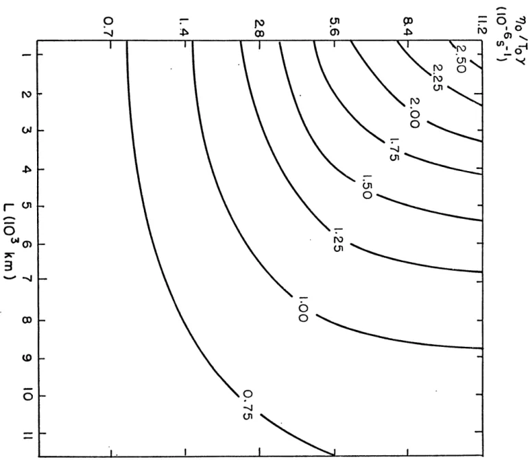
The deepening rate J,

(p

) for

T

= 1

0

C...

It Wt It

The zonal velocity component, Cx2, for the 1000 mb center. ...

Values of the northward speed, Cy3, for

- = 1*C ...

Ratio of Cx to the zonal component of the 500 mb wind ... ... ... ... ... ...

Ratio of C to the meridional component of

the 500 mb wind ... The eastward speed of the 250 mb trough and the

overtaking rate C_x(250) - Cx2 ...

The difference [ SL(250)- (1000)] for

S = L/4 ...

I 1I t'

Frictional vertical velocity over the 1000 mb

center ... Normalized square containing locations of

soundings for "before" deepening ... Same as for 10a, except for "after"

deepening ... Composite soundings for "before" deepening cases ....

II I1

Composite soundings for "after" deepening cases ...

it "I 11 20 29 30 35 36 39 41 42 43 45 46 49 50 56 70 71 72 73 74 75

Figure 13b. Table 1.

Table 2. Table 3.

Table 4.

Mean soundings for "after" deepening cases ... Calculated thickness changes over the

low center ... Values of the factor K (m/mb) ...

Calculated thickness change over the low

center ... Calculations of model parameters ...

Intense extratropical oceanic cyclones directly affect the lives of relatively few of the world's inhabitants. Nevertheless, these storms form an essential part of such semipermanent meteorological

features as the Aleutian and Icelandic lows, both of which account in part for the observed wind distribution in mid to high latitudes. They also play a crucial role, along with continental extratropical distur-bances, in the necessary vertical and meridional transport of angular momentum and heat, as has been discussed by Palmen and Newton (1969). Rapid deepening is also observed to occur more frequently in maritime storms than in continental cyclones.

In order to examine some of the properties of these disturbances, we should like to examine the results of a structurally simple diag-nostic model. Inspiration for such work comes from Sanders (1971). However, this latter model contains a temperature structure with a

hori-zontal temperature gradient decreasing vertically from its maximum value at the surface to zero at the simulated tropopause level. Since we feel this represents an inadequate representation of temperature

for maritime regions, we will use a more appropriate thermal structure. In addition, a larger range of effective vorticity stability will be used when we consider the selected properties of the model.

Documenta-tion for such a move will be made from an examinaDocumenta-tion of the vertical structure of temperature and relative humidity in areas affected by intense oceanic storms. Due to the apparent importance of friction in

the termination of deepening, a new formulation of surface friction effects will be discussed. Finally, we shall attempt to document the problem of

incorrect initial analysis with respect to oceanic cyclone intensifica-tion by examining two classic cases of explosive maritime storm develop-ment.

II. The Diagnostic Model Ha. Vertical Motion

Following the procedure of Sanders (1971), we will assume that the flow is specified by the quasi-geostrophic vorticity equation

-4 i-O U a(1)

and by the thermodynamic equation

- (2)

where is the relative vorticity,

X

₀ is a constant value of the absolute vorticity,J f , is the geopotential, and the stability parameter 6

~I/)(4

9

'

;

4

is a

function of pressure only. The relative vorticity, using the geostrophic relationship, may be expressed as

where 0 is some constant value of the Coriolis parameter. Equation (1) now becomes

Combining equations (3) and (2) to eliminate - now yields the V0 -equation.

Using a structurally simple, yet realistic profile of temperature will allow us to solve equation (4).

We assume the following thermal structure:

where x and y axes are directed eastward and northward, respectively; a 'is the intensity of the meridional temperature gradient, and

T

repre-sents the amplitude of the two-dimensional harmonic variation of temper-ature. This simplistic temperature profile does not lend itself to excessive mathematical complexity in the derivation of any forthcoming equations, and yet is quite realistic for extratropical maritime regions. Equation (5) indicates that the only variation of temperature in the vertical (with p as the vertical coordinate) is represented by the

pres-sure dependence on the mean temperature for a given prespres-sure level. Thus, there is no vertical variation of the horizontal temperature con-trast. This is approximately true over much of th- troposphere for oceanic regions. However, this temperature structiLe would extend to the top of the atmosphere, unless we specified a tropopause level, above which our temperature profile would be invalid. We shall specify this level by Pz , and disregard atmospheric processes above this

level. The price we would have to pay in attempting to realistically model stratospheric temperature (in the form of excessively complicated expressions) would presumably not be worth the additional physical

insights to be gained from such an attempt. Indeed, allowing the tem-perature structure to stray unrealistically above the tropopause, just

for the sake of defining the expression for all p, can prove to be potentially hazardous, as we shall later see.

The stability value - is assumed to be a function of pressure only, and thus will be associated with

Tr

from expression (5). The definition of 8 AI 6 , and the hydrostatic condition yields

and

with R•

Now, we define another stability parameter

where

YZ

and YO correspond to isothermal and dry adia-batic lapse rates, respectively. With 70 now chosen as a constant value of , and being. assumed independent of pressure,

the expression for 6 becomes

The distribution of geopotential at P=f' io000 mb is given by

)

^

(T4(7)

)S

9

Here, A represents the phase lag of the 1000 mb geopotential field with respect to the temperature field. A more complete explana-tion of % and 0 is given in a discussion of the original model (Sanders, 1971). Now for our "no-tropopause" case, or the horizontal temperature variation being independent of height:

where

and p is to be expressed in mb.

In order to construct an appropriate V-equation for this structur-ally simple model, we will represent the horizontal velocity V

geostrophically, as:

Using these relationships and the definitions of 6() and ))

the~J-equation (4) becomes

J

T

We will use thej -plane approximation and regard as

a constant. For example, \ . S would

correspond to a latitude of about 450.

Because of this simplified temperature field, expression (9) is a good deal less complicated than the corresponding equation in the original model (see Sanders, 1971). However, the physical interpreta-tion of the funcinterpreta-tions on the right side of (9) remains the same.

The first term represents the vertical derivative of thermal vorticity advection due to the perturbed part of the temperature field by the portion of the thermal wind due to the basic north-south temperature

gradient. The second portion of the first term involves the vertical derivative of the advection of earth vorticity by that part of the thermal wind due to the perturbed temperature gradient. The second term represents two identical effects in this model: the first being

15.

the advection of the 1000 mb vorticity field by the thermal wind due to the meridional temperature gradient, and the second is due to the advec-tion of this temperature field by the 1000 mb wind. The third and final term is the effect of the advection of the perturbed part of the temper-ature field by the 1000 mb wind.

The first term vanishes at the x-position of the temperature perturbation centers, while the second disappears at the x-position of the 1000 mb geopotential centers. The third term disappears when the. 1000 mb center coincides with cold or warm pool centers (A=-O ), at any y value corresponding to the latitude of the 1000 mb center

(y = 0), or at the latitude where no 1000 mb meridional wind component exists (y = Lq. ). Thus, it is evident that the only potential con-tribution to vertical motion over the 1000 mb center comes from the

first term on the right-hand side of (9).

We shall now divide the solution of (9) into three parts, corres-ponding to the three forcing functions mentioned above:

LJt=hW, pJ +h Le 3 (10)

with the three parts of (9) as:

(11b)

and

wUz tu::4

FI

,

L

,

(lic)

To find the solution, we require that each component of Whave the same horizontal structure as its corresponding forcing function.

So

Ua z

( (12)

and I

Now, equation (1la) becomes

(y4

J ]

t 7

JnL

(13)

Since equations (9) and (13) are second order equations, two boundary conditions are needed forJi. We will requirer0, and each of its three components, to vanish at P = Po, and P = PT. PT, as was

discussed earlier, is -some specified pressure value of the tropopause. We shall ignore all vertical motion above PT, because our assumed tem-perature structure makes no attempt to be realistic above this level. The computations performed in this paper will assume PT = 250 mb, which is a bit below the traditional vertical motion vanishing level of 200 mb. This lower level is chosen to mitigate somewhat the effect of strong forcing aloft. The solution to equation (13) is, with these boundary conditions:

N A

O W % (14)

The values of the constants shown in the previous expressions are:

where

no

' 1)

_jkT

and

Proceeding in a similar manner to find the solutions to Equations (llb) and (llc), we have

and

Subject to the same boundary conditions mentioned before, the

A A

expressions for and are

t (15)

5

bT

where

and

where

and

Each of the three components of corresponds to the appropriate forcing function on the right side of equation (9). Thus, the same physical processes are involved in the vertical motion components as are those processes described earlier involved with the forcing.

As a comparison to the vertical profile of

j

, , and VJZ found in "case C" of the original model (see figure 5 of Sanders, 1971), figure 1 shows these case C profiles for the revised model. A 250 mb

1000II I I I I I I II I .

-100 -90 -80

-70 -60 -50

-40 -30

-20

-10

0

10

20

30

40

50

60

70

80

-4

-1

w

(IO

mb sec

)

1. Contributions to vertical motion for

)~o= 0. 9 2 x 10 - 4 sec- 1 , To == 2500 K ,

"case C". _{The values of vafious parameters are / = . 114,}

L = 2900 km , = L/4.

Fig.

The general character of the profiles is preserved in both versions of the model. However, the maximum values of each of theW components is a good deal larger and occurs at higher levels than in the earlier version. The reason is that the temperature gradient does not damp out with height. Maximum values of '4 are located in the region of 500 to

650 mb in this model. It is interesting to see here how UJ (denoted

S" in the earlier version) is now the largest component,

whereas U had the largest maximum value in the original model. The reason can be readily identified from the previous discussion of the physical factors involved in producing Wit and Ql . is dependent upon both the magnitude of the basic north-south temperature gradient and the temperature perturbation, while OJ is dependent only on the 1000 mb wind field and the meridional temperature gradient (not on the temperature perturbation).

As in the earlier model, k\ gives tropospheric ascent from the cold trough to the downstream ridge, when lk > ; yields ascent from the 1000 mb low to the mb high center, while WL shows ascent north of the temperature perturbation center and descent to the

south, when . We shall later see that the dominance of Wi over \Pq, is crucial for the intensification of the low center.

While the action of vertical motion tends to be concentrated too much in the lower troposphere in the original model, our model probably

tends to concentrate the vertical motion at levels too high in the troposphere for this continental storm case. However, because our

temperature structure is likely to be more accurate for maritime cases, we should expect these higher maximum values of vertical motion for oceanic cases.

IIb. Geopotential Tendency

Suitable expressions for the geopotential tendency

may be found by solving the vorticity equation (3). This may be accomplished by finding the vorticity advection using equation (8), and evaluating the divergence term by differentiating the expression forlJ, equation (10).

The vorticity equation now becomes

(17)

where fl, f2, and f3 are simply pressure dependent functions found as coefficients of the appropriate harmonic term when deriving the above equation.

We shall divide the solution into three parts, just as the solu-tion to the W-equasolu-tion was divided

(18)

with

and

As before, we assume that each component of

the solution have the

same horizontal structure as its corresponding forcing

function, so

that

14

where

and

The evaluation of the f(p) terms yields

\wher where

,IZ\\~R~

(19)

h

s-3,

LZ ' QM

ILI

~oS ZI

"xa,

/1 (I

_-

₍₎

fcP~ia,

P+

and where

4

' PT(

b

'L -(20) where

%z

QA4-

_Q{

_{c j}

and and (21) N

\ ivlj

Ila

+ +f~P+

where ---- 4 LO

An examination of the structure of the previous terms indicates that and lA are both directly due to vorticity advection with the remaining components resulting directly from horizontal

divergence. Of course, the horizontal divergence due toW 1 is

indirectly forced by vorticity advection. Since vorticity advection effects are generally negligible at 1000 mb, the divergence represents the critical mechanism for the deepening of a 1000 mb center. Since the only vertical motion found over a geopotential center in this model is that due toVJ , negative divergence in the lower tropopause

associated with this quantity deepens the low. Thus, when a low is located between a cold trough and the downstream warm ridge, ascent in

this region due to-I intensifies the low (ignoring frictional effects).

As was discussed earlier, W\k (the ascent term downstream of the cold trough to the warm ridge) dominates rk\ (descent in the same region) to effect this deepening.

lIc. Intensification of the 1000 mb Low

If we consider the deepening rate of the 1000 mb low, where

,

O

, , equation (18) becomes

Thus, as with the previous model, maximum deepening occurs when )C/ , and the deepening vanishes when the low is located at either the cold

or warm perturbation centers. In our model,

(23)

A "case C" calculation made with equation (23) was found to be

--

,

6 - o XL or a deepening rate for sea-level

pressure of about -12.0 mb (12 hr)1. - This compares with an observed deepening of -8 mb, but we have not yet considered frictional filling. Our value for is slightly greater in magnitude than the number which would be found in the original model, even when we amplify

temperature structure in the 100 - 500 mb layer. No such amplification factor is needed in the present model, because we have assumed no varia-tion of horizontal temperature gradient with height. The reason is, of course, the enhanced forcing in the form of the temperature gradients in the upper troposphere. The physical interpretation of each of the terms in equation (23) is the same as the terms found in equation (29) of Sanders' work (1971). Both terms arise from the divergence due to

U

i . The first term on the right side of (23) arises from relative

vorticity advection, while the second acts as a result of the advection of earth vorticity. The first term is the active deepening mechanism for a 1000 mb low placed between a cold trough and a downstream warm ridge, for it produces ascent in this region; while the second term acts as a brake on the deepening process by causing descent in this same area.

Why does the active deepening mechanism have a greater effect with respect to the brake in this version of the model than in the first version? The answer is that the first term is much more dependent

on the temperature gradient magnitudes (both meridional and pertubed) than is the second term, which depends only on the perturbed temperature gradient strength (the value ). However, there is still the same superficial exponent dependence on L, as in the earlier version, such that the braking action of the second term will increase more rapidly than the increase of the first term with higher values of L. Thus, we should expect a limiting value of wavelength, beyond which no net

intensification will occur. The importance of such L-dependent parame-ters as bl and . 1 in (23) remains obscure, but is likely to be

small. Thus, discounting this latter consideration, we should expect generally higher wavelengths of maximum deepening, due to the lessened effectiveness of the braking term. We can also perceive this fact with the knowledge that since the vertical scale of the baroclinicity is larger in this model, the preferred horizontal scale is also larger in this model. Equation (23) also shows that a meridional temperature gradient is required for deepening, while

(o)

is directly propor-tional to the magnitudes of

T

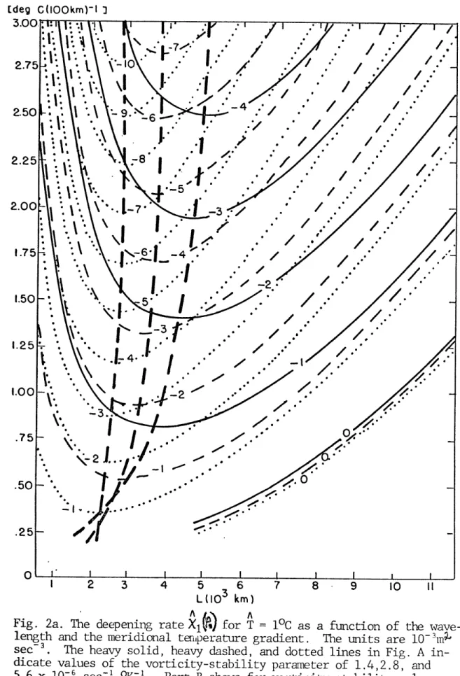
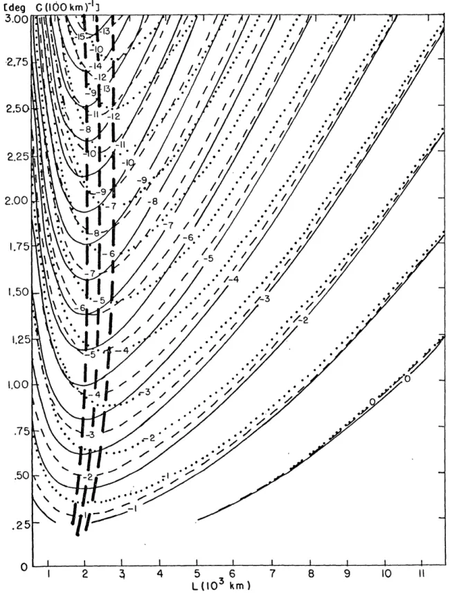
and the vorticity-stability parameter.

Figure 2 confirms and summarizes the previous statements. It also indicates that the wavelength of maximum deepening range from 1500 to 5000 km. The wavelength of maximum instability (assuming \ is an indication of the instability of the baroclinic system) decreases with increasing values of the vorticity-stability value, corresponding

with the observationally inspired notion that smaller stability favors intensification of smaller storms.

The range of both a and the vorticity-stability value are exten-ded in this and forthcoming charts from the ranges used in the reported results of the earlier version of the model (see Sanders, 1971). The upward limit of a is extended to 3.00C/100 km, because the values found in experiments conducted in a synoptic lab class at M.I.T. go beyond the previous upper limit of 20C/100. km. A maximum value of the

vorticity-stability parameter of 11.2 x 10C 1 sec is chosen on the basis of a high value of N~: = (area averaged), T = 250,4'4 YZ.[+4 This latter value is taken from the least stable saturated sounding

(with respect to the moist adiabat) of a sample of radiosonde obser-vations (mainly weather ships and island stations) in regions under the

29. Edeg C(IOOkm)-I ) 3.00-1:1:1 rl t -I 2 3 4 5 6 7 8 - 9 10 II L (103 km) A j\ A

Fig. 2a. The deepening rate X1 for T = 10C as a function of the wave-length and the meridional temperature gradient. The units are 10-1"m

sec - . _{The heavy solid, heavy dashed, and dotted lines in Fig. A}

in-dicate values of the vorticity-stability parameter of 1.4,2.8, and

5.6 x 10-6 sec-' o_{K -} . Part B shows for vorticity-stability values of 5.6,8.4, and 11.2 x 10- 6 sec-' OK-' for the dotted, lightly dashed,

[deg C(IOOkm)- 3 3.00 -15 * / / / . / .\1 t\ t

1

-10 */ 2.75 * . /**/ * . .9 / / , ., /1 .. 2.50 " "-1. // .

/

/

.

./

2.00 -8 1.75 - , .. .*/ .*1

. *\

.;.

.,

....

;/"

*,

,

g

.

-/-4

1.50

*/\

/. / . * . */ ./ * ,*/ .*

1.25

.

.

/

.

-5*p 1.00 .50 .25 0-I 2 4 5 6 7 8 9 10 11 L(IO3 km)

Fig. 2,. and lightly solid lines, respectively. The extra heavy dashed lines connecting the troughs of the isopleths are the loci

influence of intense oceanic storms. Due to our previous assumption of

Y

being independent of height, this stability value necessarily is based on a deep layer. Temperature differences between 850 and 500 mb are used in determining

Y

. Thus, boundary layer effects and vertical temperature differences above 500 mb are not considered. Latent heat of condensation can be taken into account in saturated layers, if the vertical temperature difference is compared to the vertical temperature difference along the appropriate moist adiabat. Therefore, the extension of the vorticity-stability parameter to higher values represents an attempt to consider the effectively lowered static stabilities when the air is saturated. This consideration will hopefully lead the model to capture some of the explosive development which is so frequent over maritime regions. A more complete discussion of the stability sampling

is contained in a later section of this paper.

One further note concerning the notion of a longwave cutoff is added here. An original attempt to define a temperature field of the form

(24)

was used to specify still another set of model equations. Equation (24) shows that the magnitude of the temperature gradients do not damp out as much with height in the troposphere as do the gradients in the original model. However, the price paid for such a benefit was an even more unrealistic stratospheric temperature profile in the form of excessively large horizontal temperature gradients. The upper boundary condition to the. -equation was VJ = 0 at p = 0, as in the original version of the

model; these latter two effects brought on an unrealisticU_{I 1} profile (especially in the stratosphere), and, thus, potentially spurious \ values. This latter event manifested itself at 1000 mb, and was readily

seen when a chart of the form of figure 2 was constructed. We found that for increasing values of the vorticity-stability parameter, contamination from excessive forcing from the region of the atmosphere above the tropo-pause increased so that a longwave cutoff for deepening no longer

existed. At./

)

values high enough (say, at -=

2.8 x 10 60C-1 sec- ), the deepening rate actually increased with wave-length, apparently without limit.

This trend is even evident in Sanders' figure 13 (1971), but not nearly so much because the excessive forcing is not as great. Contamin-ation appears at wavelengths greater than 6000 km by virtue of the slope of the lines decreasing with increasing values of ( .

Pre-sumably, if the values of were computed for much higher (and

beyond the range observed in the real atmosphre) values of the vorticity-stability parameter, no preferred wavelength for invorticity-stability would appear, as in the situation described above.

IId. Motion of the Features

It is of interest to examine the motion of the geopotential features. We need simply use Petterssen's (1956) formulas to evaluate the motion. The eastward speed may be written as

)x ) (25)

The position of the trough axis, XT, may be found by looking for the minimum value of geopotential (x, y, p), along the y = 0 axis. The solution is

where XT is between x = 0 and x = (L/t ) - , the position of the 1000 mb low. We may now find an expression for dXo , with a knowledge

of) T by differentiating our expression for once and the one for

(x, y, p) twice, so that

L7

For the motion of the 1000 mb low center, equation (27) may be expressed as

where '\ and 6 represent the effects of , and respectively: (29) and

I

(30) 0

For our sample case, the values of L and | in this version of the model are 17.4 m/sec and 9.3 m/sec, respectively. This compares with 14L = 13.7 m/sec and kl = 4.7 m/sec in the old version. The observed 12 hour displacement rate was 11 m/sec, showing the new calculations as being too fast. The parameter Qj is still smaller than ty , but represents a relatively greater significance with respect to tp than in the old formulation. The reason is the new temperature profile enhances

]

more than . has

no effect if the low is located so that = L/$y , as happens in our sample case C. The physical effect of !4d is the same in this model version; it will retard eastward speed for warm lows and enhance it for

L/

<L/ . Since 4I has a potentially significant effect in the model, accurate placement of the low (to determine

X

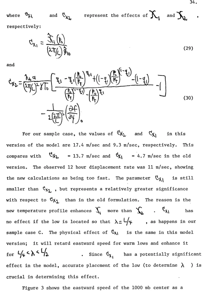
) is crucial in determining this effect.

Figure 3 shows the eastward speed of the 1000 mb center as a

35.

a )-I

Edeg C(100km) I

I 2 3 4 5 6 7 8 9 10 II

L (103 km)

Fig. 3a. The zonal velocity component, Cx2, for the 1000mb center as a

function of wavelength, and meridional temperature gradient for selected values of vorticity-stability. The isotachs indicate units of meters per second and are positive values for eastward displacement. The

corres-pondence of the solid, dashed, and dotted lines in each part of the fig-ure are as explained in figfig-ure 2.

L (103 km)

Fig. 3b. Same as for part A, xcept for vorticity-stability values of 5. 6 , 8. 4, and 11.2 sec 1K.

a

values of this motion are found in the wavelength range from 2500 km to 8000 km - somewhat higher than the wavelengths found in Sanders' figure 10 (1971). Also, generally higher westerly values for a given vorticity-stability parameter, wavelength, and a value are observed in this formu-lation. Increasing magnitudes of eastward movement are found with

increasing vorticity-stability numbers and increasing a values. The wave-length of maximum speed decreases with increasing values of vorticity-stability , juist as the wavelength of maximum deepening decreases with higher magnitudes of vorticity-stability. The reader should be cautioned to watch out for the effect of Nt , particularly when the temperature perturbation is intense; because the magnitude of Ox| is direclty proportional to

T

The meridional component of motion may be obtained by using Petterssen's formula:

Cl

z

(t4.-x~)

~

(31)

so that

(32)

where is due to and

J1% P.I

₍₄

1'i

I

~-

~iia-L?

t j~ti

\Lj "

-C94,

Since tl3 is generally a positive term, geopotential centers have a northward component of motion when located between the cold trough and its downstream warm ridge. The case C value of Il is 10.2 m/sec, compared with the earlier model value of 9.1 m/sec, and an observed 12 hour displacement rate of 7.5 m/sec.

Figure 4 shows values of.61 for i = 1C as a function of vorticity-stability and wavelength. The magnitude of

Cy

3 is

pro-portional to the magnitude of

T

,and independent of the basic meridi-onal temperature gradient. The main difference between this figure and Sanders' figure 11 (1971) is that values for larger values of vorticity-stability are given here. There is a slight increase of 3 over corresponding values in the earlier version, for given values of L and

A comparison of the motion of the low center with the flow aloft at 500 mb is appropriate. We have seen that the zonal motion of the 1000 mb low ( CXL ) is due to the divergence of Wf , which is forced by the meridional temperature gradient; while the meridional displacement of the feature is due to the divergence of aJ , which is forced by

the temperature perturbation gradient. Although the contours of the 500 mb pattern are associated hydrostatically with the above temperature patterns in the 1000 - 500 mb layer, a direct steering relationship between the flows at 500 mb and the 1000 mb low is not clear.

39. 0 Q| 0

ro

O rio

nn

OD 0

00

_NO

<o

-Fig. 4.

Values of the northward speed C,3 as a function of

vorticity-stabil;ity value and the wavelength for

= 1

oC.

The isotach labels

are in units of meters per second.

From our definition of f (x, y, p), equation (8), and for \-Z

t(33)

V

if

~I

(34)

For case C, we find values of U5 = 24.1 m/sec and V = 33.8 m/sec. The values of C and C are 17.4 m/sec and

x2 Y3

10.2 m/sec, respectively. Thus, the low is moving at a speed of 20.2 m/sec toward 0600 while the 500 mb flow is 41.5 m/sec toward

0350. When a comparison is made with the earlier version of the model,

we see that the low is moving somewhat more to the right of this 500 mb flow in this version. The speeds of both the 500 mb flow and the low are greater in this model (20.2 m/sec versus 16 m/sec for the low, and 41.5 m/sec versus 31.2 m/sec at 500 mb), due primarily to the enhanced

temperature gradients aloft.

The relationship between the 500 mb flow and the 1000 mb system movement is shown in Figures 5 and 6. The ratio Cx2/U5 has maximum values at wavelengths between 2500 km and 8000 km for a given value of a , and for the indicated vorticity-stability range. Also,

for given values of a, '~ , and L, Cx2/U 5 tends to be

slightly higher than in the previous model. Values of Cy3/V5

a

[deg C(IOOkm)13

I 2 3 4 5 6

L (103 km)

7 8 9 10 II

Fig. 5a. Ratio of Cx2 to the zonal component of the 500mb wind as a

function of meridional temperature gradient and wavelength. The sol-id, dashed, and dotted lines in each part are as indicated in Fig. 2. The heavy dashed lines indicate the loci of wavelength, beyond which the 1000mb low pnoves to the left of the upper level flow.

3.00 .rr1. ;-n

I 2 3 4 5 6 7 8 9 10 11

L(10 3 km)

Fig. 5b. Same as for 5a, except for vorticity-stability values of 5.6,8.4, and 11.2 sec- 1 _OK-1.

(10

6 -

S

- I

)

11.2 .

8.4

5.6

2.8

1.4

-0.7

I

2

3

4

5

6

7

8

9

10

II

L ([0

3

_{km )}

meridional component of the 500mb wind as a function of wavelength and

Fig. 6. Ratio of Cy3 to the

from the extension of the range of vorticity-stability values, little change from Sanders' figure 12 (1971) is indicated. We see in figure 5 that the conditions under which lows move to the right of the 500 mb flow are those under which most storms are observed to occur (for

A- L/q

, the low moves to the right of the 500 mb contour when SV ). Indeed, a somewhat wider range of conditions under which this movement occurs is found in this model. As in the earlier model, both the 500 mb flow and the motion of the low approach the zonal direction when the surface feature is located at either of the temperature perturbation centers.

Since the 1000 - 500 mb thickness pattern is shaped in a similar fashion to the 500 mb pattern, the theoretical and observed motions of surface lows generally moving to the right of the 500 mb flow indicate that they also move toward warmer air. However, this does not mean that the low is warming, because the adiabatic ascent over the cyclone acts to oppose the warm air ingestion of the storm. The topic of thickness change following the low center will be discussed in a later section.

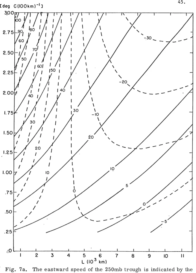
We shall now examine a possible clue as to the extent that occlusion takes place in the model. If the 250 mb trough were over-taking the surface low, the cold perturbation would presumably be doing likewise; thus, occlusion would be occurring. Since the zonal speed of 250 mb trough is a complicated function of all the model parameters

(see equations 26 and 27), figure 7 shows the results of calculations

OW- _{& 32 -2}

for

-

= 50C, Q = 10 m sec-, and with b/Y,

-6 -1s -1 an 6o -1 -1

45. [deg C(IOOkm) - 3 3.00!,/ ,I I -r

2.75

2.50

2.25

2.00 1.75 -

I

-i I I 30 1.50 I I I 20 1.25 / /

I

I1

1 1.007 / 10 I 5 .75- /

/o

.50 - / -5 .25 I 2 3 4 5 6 7 8 9 10 L (103 km)

Fig. 7a. The eastward speed of the 250mb trough is indicated by the solid lines, while the dashed lines indicate the overtaking rate,

Cx (250) - Cx2, as a function of meridional temperature gradient and

wavelength. Part A of the fig. is for o/To = 2.8 x 10- 6 sec - 1 oK-l T --5 OC, and = L/4.

C(100 kmi 1

I 2 3 4 5 6

L (103 kim)

7 8 9 10 II

indicates the same parameters except for

Io/T

sec-1 OC-1

[deg 3.

Fig. 7b.

11.2

Part b

x 10

- 6

of figure 7 may be compared directly with figure 16 of Sanders' work (1971). We see that, although the overtaking rates are much higher in this model for certain high a values and small wavelengths, that an overtaking rate of about 5 m/sec is indicated for the wavelengths of maximum deepening (see figure 2). This is quite similar to the results

found in the earlier model. A look at part B of figure 7 shows for this larger vorticity-stability value that for the maximum deepening wave-lengths, the overtaking rate for a large nuaber of a values is only about 2 - 3 m/sec. The fact that significant deepening of the storm can occur without the tendency to occlude (see figures 2 and 7), along with the

trend of the less overtaking by the 250 mb trough with increasing values of vorticity-stability, points to the likelihood that some other process cuts off the storm intensification. A sampling of rapidly deepening storms found in a synoptic lab class at M.I.T. showed no clear trend to occlude. Thus, friction, which has yet to be considered, might be

expected to cut off the deepening of a storm, rather than the process of occlusion.

lie. Temperature Perturbation Tendency

Now, we wish to consider the rate of intensification (or lack of it) of the temperature perturbation. The tendency of the thickness of the 1000 - 250 mb layer at the cold trough (x = 0, y = 0) is

-~

~

[ ( )(35)

From our expression for , we have

41

j

(36)

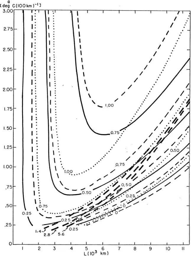
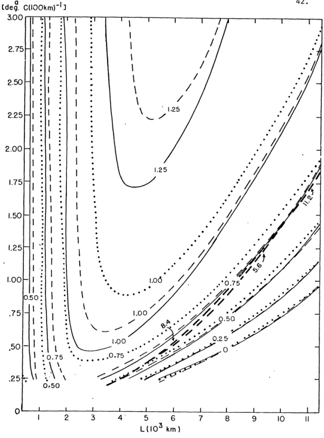
Equation (36) indicates a different wavelength dependence in each of the two terms on the right side, so that a critical wavelength is indicated, below which no intensification will occur. Because this dependence appears similar to the expression in Sanders' equation 40

(1971), we. should expect a similar pattern of thickness tendency in our calculations to those of Sanders' version. Figure 8 shows these patterns, but we also see a major improvement over the earlier formulation. That is, for each vorticity-stability value and for (0 4 X4 L- ), the wavelength of maximum deepening is also a wavelength at which the

[deg. C(100 km)-FI 300 i I .r2. 49. 1.00 . o ..l .75- 5 .

j*"

.5.o '." "

0"

.50-

_G.

.25

.:,

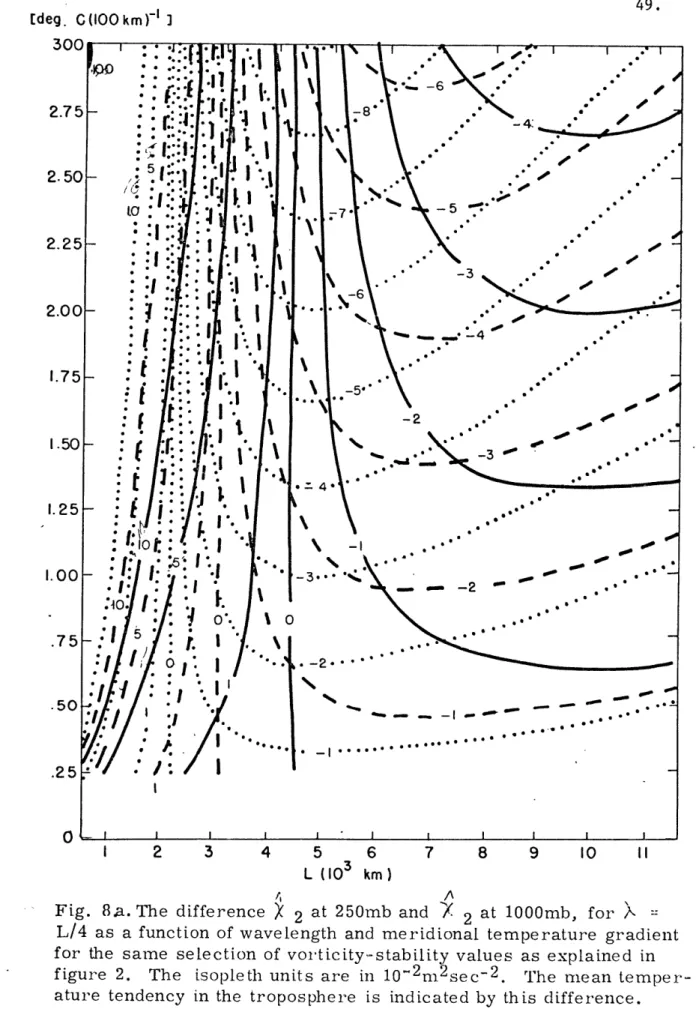
0 I 2 3 4 5 6 7 8 9 0 L (103 kin) = A

Fig. 8.a. The difference 2 at 250mb and / 2 at 1000mb, for A L/4 as a function of wavelength and meridional temperature gradient for the same selection of vorticity-stability values as explained in figure 2. The isopleth units are in 10" 2_m2_sec- 2_{. The mean} temper-ature tendency in the troposphere is indicated by this difference.

[deg C(100 km)-'1.

300i 1I11 11 I1 1

I 2 3 4 5 6 7 8 9 10 11

L(10 3 km )

Same as for 5a, except for vorticity-stab

and 11.2 sec

- 1

OK-1 .

ility values of

Fig.

5.6,

8b.

8.4,

the first version of the model. By examining figures 2 and 8, we see

5 1 AL0-10-1

that for a = 2.0 x 10-5Cm andA~ = 2.8 x 10-6 sec- K , the temperature perturbations are intensifying at around 2.0 *C/12 hours for the preferred wavelength of deepening. As the vorticity-stability

parameter increases, there appears to be a tendency for this intensifi-cation rate to increase for the wavelength of maximum deepening. Thus, with this version of the model, which tends to be especially realistic for maritime cases, the intensification of the storm actually occurs simul-taneously with the intensification of the temperature perturbation. That is, zonal available potential energy is converted to eddy available poten-tial energy in this model, as deepening occurs.

IIf. Frictional Effects

A calculation of the filling rate of a storm due to friction necessitates an understanding of what the frictional force is at the ground, and also how it acts above the surface. Rather than specifying a cross-isobaric flow and a lower boundary value of (due to friction) at the top of the surface friction layer (see, for example, Sanders,

1971), we shall make an attempt to find an analytic solution to the equation with frictional forcing

Cr7) w VX (37)

6

where is the vertical motion due to frictional convergence or div-ergence, and is the frictional force vector per unit mass. The solution to (37) depends, of course, on how we specify F ; and if we define

F

to be linearly proportional to the 1000 mb geostrophic velocity vector, analytic solutions may be found. Haltiner (1971) finds the vertical motion at the top of the boundary layer using both a linear relationship, and a (velocity)2 dependence. Of course, the latter depen-dence would be preferable, but solving the W-equation would become much less manageable. If we further assume that the frictional force acts in an opposite direction from this wind vector, then

1-1

&Voo

(38)

Further, it is physically reasonable to parameterize the frictional force such that it is a maximum at the ground, and damps off exponentially with height, so that it becomes '(|/i ) times its 1000 mb value at the top of the surface boundary layer (say, at 900 mb) and vanishes at p = 0. Thus,

(w' - .(39)

where C_d is the surface drag coefficient, Vo is a specified value of the 1000 mb wind (independent of horizontal position), and

6.

is the depth of the boundary layer (usually about 1 km and corresponding to the pressure scale height of 900 mb). Thus, at 1000 mb, the frictional force per unit mass is

We see that

&

is proportional to the square of the velocity, at least superficially. The limitations here are that

V

will be a rather large overestimate of the 1000 mb wind in a cyclone, while

V

is a constant value defined for the region at 1000 mb under the influence of frictional convergence of divergence. Although the specified value of

V

appears to be the most serious limitation of our formulation, somewhat less ad-hoc decisions must be made for the values of d

Mindful of these foregoing liabilities, we shall proceed now

with the business of finding a solution to (37). The 1000 mb vorticity may be expressed geostrophically as o

, where, as before

kU

so that

11

#:

L

M(

Now, equation (37) becomes

If we assume that W4, has the same horizontal

structure

forcing, set the boundary conditions as W = 0 at p

= p and p

solve analytically for the homogeneous solution,

and approximate

the particular solution by a Taylor's series,

then the solution to

is ___

±L

F

xQ&'~hih~a

where

(40)

is its = 0,

(40)

(41)

55.

and

The reader might reasonably ask why we did not set the upper boundary condition of W* = 0 at p = PT , as was done with the other

components of WJ . The answer is that the frictional forcing is parameterized to be small enough at higher levels, so that Jis virtually negligible at the tropopause level anyway. This fact is

quantitatively shown in figure 9, where a vertical profile of U . over the surface low is shown for the parameter of our sample case C. A

-3

drag coefficient of 2.0 x 10-3 (a typical land value, see Cressman, 1960), V = 10 m/sec, and = 1R, 1 km were used in the computations. We see

that the maximum value of Wt is found at about 850 mb, with an expo-nential-like decrease above this level. The values are somewhat less

than the largest components of vertical motion found in figure 1, but still will be important when we consider the effect of convergence and divergence in the height tendency. The W -profile shown in figure 9 shows what we would qualitatively expect from quasi-geostrophic theory with the convergence confined to the lower troposphere and the divergence

P(MB) 0 50-100 150 200 250 300 350 400 450 500 550 600 650 700-750 800 850 900 950 1000 iii tl i -13 -12 -II -10 -9 -8 -7 -6 -5 -4 -3 -2 -1 0

W4 OVER THE LOW (10- 4 mb sec- )

Fig. 9. The frictional vertical velocity over the 1000mb center with units in 10- 4rnb sec- 1 case C.

57. The 1000 mb height should be rising, because the larger dissipative effect of friction exceeds the tendency of the convergence in the lower layers to cause the heights to fall. We need to look at the height tendency equation to verify this fact.

The -equation due to the forcing by frictional dissipation and divergence may be expressed as

-O

(42)

where < is the height tendency due to the frictional effects on the right side of (42). If we regard t as having the same x and y dependence as its forcing functions, then

Nu-.~~"l~~m ₍₄₃₎ where

4z

4

htc

(X

~~~kl)

R71

The last term above represents the effects of frictional dissipation, while the other terms are the result of the divergence of LW, . At the low

center, x = , y = 0, and the signs of each of the terms in the

4

expression are reversed so that we can see physically that the dissipation term represents a height rise, as expected. Using the same numbers as above for , A ,and L ,we find the 4 value

-4 2 3

over the low for case C at 1000 mb is 61 x 10 m /sec , which corresponds to a filling rate of +3.6 mb/12 hours. This, when combined with our fric-tionless deepening of the case C storm (-12.0 mb/12 hours), yields a net intensification of -8.4 mb/12 hours - quite close to the observed rate of -8 mb/12 hours. Our computed value of ( '\ ) is much closer to the

observed number than the figure found in the original model version.

A A

Whether this is due to a better formulation for o , or\ is not clear; the magnitudes of both numbers are larger in this model, and it is exceedingly difficult to successfully "observe" the frictional filling rate in the real atmosphere.

The parameter q1 1 increases with decreasing wavelength with

all the other input values being held constant. However, it is not immediately clear from (43) how

S

behaves as L decreases. Indeed, as in the previous model, the filling rate does increase with decreasing L, providing for a shortwave cutoff, assuming 0

40

. We also have a limiting intensity established because is independent of 0 , while is directly proportional to it. Using 010 = 1020 m (sec)- 2 for

the sample case C, the limiting intensity may be expressed as

59. 3 2 -2

For our sample case C, this value is 3.43 x 10 m sec , The range of sea-level pressures that this value corresponds to is about 93 mb. This increased value over the earlier results is due to generally greater increased values of 1\ than U .

III. Experiments with the Frictional Expression

As a check on the reliability of the aforementioned frictional formulation, we examined some cases of rapidly deepening cyclones over the North American continent, where surface analyses indicating the deepening rates and evolution of the cyclone structure are more reliable than over the sea. The 1000 - 250 mb thickness analysis is presumably accurate in land areas, where upper air observations are sufficiently dense to achieve this accuracy. Specifically, an experiment was under-taken to check on whether our frictional formulation is sufficient to account for the observed thickness change over the center.

Reference is made to the discussion given by Sanders (1976). The quasi-geostrophic vorticity equation for flow at sea-level is

S

tV

S

where the subscript SL refers to sea-l1vel,1j o is a constant value of absolute vorticity for the appropriate domain, and is the frictional

force per unit mass as previously defined. The advection term disappears at the center of the cyclone. The relative vorticity is given as

where pL_ and t are both regarded as constant values of the sea-level density and the Coriolis force. The harmonic variation of

where b is the semi-amplitude of

a

, and L is its wavelength. Now, our vorticity equation becomes an expression for the central

pres-sure tendency, SLi t , and by assuming a linear structure of

with height from a zero value at 1000 mb to its maximum at 600 mb, we have

4t

-Q

r-)-

(44)

This latter assumption may not be too accurate if the storm is quite intense, and the components of the frictionally induced vertical motion becomes larger, resulting in a maximum Wk below 600 mb. Thus, in this, the sea-level divergence would be assumed to be larger by

de-creasing the denominator above (the pressure difference through which

W increases to its maximum).

Defining ' , we will use as a typical

domain averaged value of the sea-level wind velocity, and use the -2

same numerical value as before: Cd = 2.0 x 10 , V = 10 m/sec, and 6L. = 1000 m. The equation for the local rate of change of thickness (in the 1000 - 500 mb layer) a y , ignoring diabatic effects and differences in the surface boundary layer (where W\ is small, anyway), may be expressed, according to Sanders (1976) as

(45)

Equation (45) represents adiabatic effects due to vertical motion on the thickness change, (s ) indicates the average of this value in the layer and will be taken as a constant value 92 . Now, we proceed to eliminate WJ between equations (44) and (45), by expressing P).

in terms of S and from the ideal gas law, and assigning -4 -1 typical values to the following parameters: f 0 o = 10 sec-TSL = 2730K, = 1000 mb. Thus, expressing L in thousands of km,

we have

(46)

If the layer under consideration is saturated, then we should take into account latent heat release by expressing the stability in terms of the moist adiabatic lapse rate. Thus (- - ) would be

replaced by ) - (- )[( )A ]. So, in this case, we have

(47)

Equation (47) shows that the static stability is effectively reduced for the moist case. The physical significance of both equations

(46) and (47) is that convergence at the surface, which increases the vorticity and causes central pressure falls, also adiabatically cools the layer above through upward motion, when the atmosphere is stable. There is an additional frictional effect, which implies that the thickness decreases locally with cyclonic vorticity due to frictional covergence and the resulting upward motion.

The first and second terms of (46) and (47) were isolated and evaluated for the various cases to determine /a+ . However, we must also take into account the movement of the storm toward warmer or colder air. Thus, if the storm is moving with a velocity vector , the local thickness change following the center may be

expressed as

\FT11(48)

Generally, the surface cyclone moves to the right of the upper level flow and thus toward warmer air (see Sanders, 1971). So the local change of thickness over the center is usually due to the opposing effects of movement to higher thickness values and cooling due to adiabatic ascent.

A balance in equation (48) is sought in the sampling of land cases, using the frictional term in (46) or (47). First, however, we should make this procedure more applicable 'to the standard 12-hour time interval.

found between map times. A similar procedure is discussed in Sanders (1976). From equations (48) and (46) or (47), depending upon whether we wish to use a dry or moist process, we integrate (48) over a twelve hour period and

find that -~

where

for moist processes, and

for dry (unsaturated) air, where 6 is the local 12-hour thickness

change over the cyclone center in a coordinate system fixed on the earth's surface (which can be obtained from the 12-hour change of the central

pressure and from an appropriate static stability value), and ( Af )

is the 12-hour thickness change following the center in a coordinate system moving with the center, which is what we would like to determine. The integrated value of 6*9 over the 12-hour period may be

approxim-ately expressed as . = 6/ ,where is the length

of the 12-hour displacement vector with a speed C. Thus,

where and .( are the times at the beginning and end of the 12-hour period, respectively. Now, we can approximate h by taking the average of the thickness differences between the upstream and

downstream ends of the displacement vector for the cyclone, at the begin-ning and end of the twelve-hour period. Thus

'(49)

so that now equation (48) becomes

(50)

As has been pointed out by Sanders (1976), since we need know only

the thickness values at the (

) and (

4(

) points, any errors in the

thickness values near the low center will not contaminate the thickness analysis significantly at these latter mentioned points. In practice, the analyst would know from the surface and upper level analysis 12-hour earlier, iy , , and ; . These current analyses would indicate E and . Now, taking

= ~PS '

=--,

L

, appropriate value of

the static stability, and using the appropriate values of Q , Vo ,

and 4, , we can estimate a value of ( 4 ), and therefore of ,

the desired value of thickness over the low center at the current time. This procedure has been formulated for oceanic areas where there is

likely to be a problem in knowing the value of the thickness, over the center, due to the likely small number of aircraft observations and

satellite soundings, which will disclose only the large scale upper level patterns. Thus, if a ship's observations disclose the presence of a small intense cyclone near the surface, a likely overestimate of the thickness over the low center will result.

Using the procedure described above, we did some calculations of

( b ) for rather intense cases over land, where the thickness analysis is likely to be fairly reliable. Thus, we have somewhat of a check on our procedure before we attempt to use it over oceanic areas. These cases were chosen in mainly the north central part of the United States, where

6 values are likely to be around 2.0 x 10- 3 (Cressman, 1960). Thus,

-3 ₌₁

/e

4

was evaluated at 2.0 x 10- 3 i = 1000 m, and

Vo

= 10 m/sec for these cases. Four calculations were made for each of the time periods used in these cases: those of dry processes with and without friction and those of moist processes with and without friction. By "with and without friction", we mean including and not including the second term on the right-hand side of (50) . The values of

k

, or equivalently, the static stability, were deduced from mean temperatures near the surface center at 850 and 500 mb. The numbers are summarized case by case in Table 1.

The time periods with an asterisk next to then indicate that the moist process was judged to be the relevant process taking place by virtue of the air being near saturation at both 850 and 500 mb. In the other cases, the air over the low was generally saturated at 850 mb, but at 500 mb, some drying out had taken place; so, unsaturated air was evident due to the dew point depression being at least 40 K.

Thus, in the latter instance, we should expect that an observed thickness change over the center would be predicted by a value somewhere between our moist and dry with friction calculations. We see that for

the moist cases, our moist with friction predictions are generally closer to the observed value than those predictions without friction. We note

Table 1

Calculated Thickness Changes over the Low Center

(Case of October 24-25, 1975) * 00Z, Oct. 25 -12Z, Oct. 25 * 12Z, Oct. 25 -00Z, Oct. 26 * OOZ, April 3 -12Z, April 3 * 12Z, April 3 -00Z, April 4 00Z, March 4 -12Z, March 4 * 12Z, 00Z, Jan. 13 -Jan. 14 OOZ, Jan. 14 -12Z, Jan. 14 0 -133 39 + 28 +122 + 60 - 70 +210 +130 +250 (Case of April 3-4, 1975) - 60 -475 - 22 -158 +100 0 -332 + 38 -108 +100 (Case of March 3-5, 1974) -240 -400 - 18 - 36 + 44 (Case of January 13-14, 1976) - 40 -224 - 58 - 46 + 12 -110 -204 + 28 - 60 + 54

generally that since the low moves tcward warmer air, the manner in which the air is cooled over the low is due to intensification and to friction-ally induced upward motion.

On the basis of our results in Table 1, we feel that our frictional parameterization does a reasonably good job of helping to account for observed thickness changes over the low. Without this frictional effect, a calculation of thickness tendency would likely not cool the low suffi-ciently to correspond with the observed change.