Does Property Market Risks Matter in Commercial Mortgage Loan Pricing: An Inquiry Into the Determinants of Commercial Mortgage Loan Spread
by Xin Wang
Bachelor of Economics, Central South University 1997 Master of Management, Central South University 2000
& Hongfei Chen
Bachelor of Engineer, Huazhong University of Science and Technology 1992 Master of Landscape Architecture, Pennsylvania State University 2000
Submitted to the Department of Urban Studies and Planning in partial fulfillment of the requirements for the Degree of Master of Science in Real Estate Development
at the
Massachusetts Institute of Technology September 2007
© 2007 Xin Wang & Hongfei Chen. All rights reserved.
The author hereby grants to MIT permission to reproduce and to distribute publicly paper and electronic copies of this thesis document
in whole or in part in any medium now known or hereafter created.
Signature of Author _________________________________________________ Department of Urban Studies and Planning
July 30, 2007
Signature of Author _________________________________________________ Department of Urban Studies and Planning
July 30, 2007
Certified by _________________________________________________ William C. Wheaton
Professor of Economics, Department of Economics, Thesis Advisor
Accepted by _________________________________________________ David M. Geltner
Does Property Market Risks Matter in Commercial Mortgage Loan Pricing: An Inquiry Into the Determinants of Commercial Mortgage Loan Spread
By
Xin Wang & Hongfei Chen
Submitted to the Department of Urban Studies and Planning on July 30th , 2007 in Partial Fulfillment of the Requirements for the Degree of Master of Science in
Real Estate Development
Abstract
The study takes a quantitative approach to test the determinants of commercial mortgage loan pricing at origination. The determinants include capital market risk, property market risks, mortgage terms and property characteristics. Taken into consideration of the endogenous factor between loan spread and LTV ratio, we use the OLS and 2SLS model to examine the variables of driving the spread and LTV and the interaction between them. The conclusion is drawn that there is little linkage between property market risks and commercial mortgage loan spread at
origination. Therefore, commercial mortgage is mispriced in terms of property market risks.
Thesis Supervisor: William C. Wheaton Title: Professor of Economics
Table of Contents
Abstract... 2
Table of Contents... 3
Acknowledgments... 4
1. Introduction... 5
1.1 Commercial Mortgage Lending and Associated Risk Factors...5
1.2 Objectives of Current Study………..……….7
1.3 Executive Summary……….………..8 2. Literature Review... 10 3. Methodology ... 18 4. Description of Variables... 25 5. Data Overview………... 28 6. Empirical Results………...…... 31 7. Interpretation of Results ... 40 8. Conclusion………... 49 Bibliography ... 51 Appendix... 53
Acknowledgments
We are extremely grateful to our advisor Professor William C. Wheaton for his guidance, knowledge and sharp insights. Dr. Wheaton has the unique ability to pass on his in-depth knowledge and lend unique perspective to our research. We thank him for leading us to the ‘cutting edge’ and beyond.
We would like to thank Sally Gordon at Moody’s for her valuable input on the topic. Her previous research paved the road for our current work. Without her contribution, this study would not have been possible.
We would also like to thank Professor David M. Geltner for his advice at different stages of this research. We are also thankful to Leslie Kizer at Moody’s for her assistance in providing the data. Most importantly, we would like to thank our families for their endless support and
1. Introduction
1.1 Commercial mortgage lending and associated risk factors
Currently, there are more than a trillion dollars of commercial mortgages outstanding and the market is still growing, both in the United States and around the world. Investigating the
determinants of commercial mortgage loan pricing has become the center of many researches on the academic level as well as in the investment industry.
As one important impact on commercial mortgage rate is the development of CMBS market. It has provided additional liquidity to the CRE market and tied the property market closely to the capital market. As an alternative source of financing, the CMBS market also increases the competition and forces the lender to loosen terms on commercial mortgages in order to stay competitive. This in turn leads to a highly corresponding effect between market risks and conduit loan pricing.
In fixed-rate CMBS conduit loan, initial loan pricing is important to debt investors because it decides the returns debt investors will get over a long period of time. Debt investors are different from equity investors in terms of an inherently asymmetrical position: they suffer more from the downside than they can benefit from the upside of market movement. Therefore, if property market is going down, higher spread should be required by debt investors to compensate the one-sidedness and scale of market risk.
Meanwhile, in practice, loan pricing depends on credit risk assessment. Some approaches of analyzing credit risk, whether corporate or commercial real estate, assume that most if not all of the relevant market information is embedded in initial loan spread. Therefore, variance in property market performance as one of the most significant factors in credit risk should be reflected in mortgage pricing.
In theory, loan pricing should reflect the future market risk as mortgage loan will be paid off by future cash flow from underlying property which is subject to impacts of future market
conditions. But we noticed that most of the investors make decisions based on past or current events.
In addition, the noncredit risks, such as those associated with the prepayment, are not part of the study, and commercial mortgage studied are not pre-payable without substantial penalties. For debt investor, the stable property cash inflow yield long term return before the final balloon payment. It is likely that the profitability of the property is more important than its value changes over the years.
Quantifying the credit risks of the CMBS conduit loan has been the focus of fixed income research. Our research will zoom in the most important risk factors in property and capital market, from the perspectives of lender and borrower, to investigate the impact on commercial mortgage pricing.
1.2 The objectives of current study
The relationship between market risk and the loan spread is broadly studied in previous research. Although the determinates of mortgage risk premium has been identified in overall market as well as for specific market segment and product type, the interaction in between the risk factors has been left unexamined, and the effect of such interaction derived from the lender / borrower relationship is scarcely studied.
Based on previous study and an interview with Bob Brown, a senior specialist of commercial lending at Key Bank, Boston, LTV ratio is an endogenous factor that depends largely on the negotiation between lender and borrower, as well as the loan spread. In order to identify the role of each factor that drives the loan spread, the current study undertakes the following approaches:
• Use the econometric tool to identify the quantitative relationship between loan spread and risk factors
• Use supply/demand market equilibrium model to explain the interaction between risk factors and loan spread
• Use loan spread and LTV as dependent variables to run two pass regression in order to minimize the endogenous factor between the relationship of loan spread and LTV ratio
1.3 Executive Summary
The study identified the endogenous relationship between LTV ratio and loan spread. Further to eliminate the effect of the factor, joint reduced form estimated by OSL regression and 2SLS regression are performed. The results of the two methods have been consistent and summarized as followings:
The origination loan spread is determined by Treasury rate, loan maturity, property size and age. The property market characteristics do not impose strong impact on loan spread for most of the property types.
The determinates show consistency with their impacts on loan spread across different property types after considering the endogenous factor of LTV ratio and spread.
Property market risk, which represented by three variables: standard deviation of property market change, correlation of NOI or value appreciation between sub-market and national
market, and historical and future property market change, doesn’t show consistent and significant impact on loan spread among different property types.
The property characteristics drive borrowers’ demand; mortgage characteristics drive lender’s supply; capital market characteristics drive both demand and supply. However, property market characteristics appear to drive neither the loan demand nor supply. Although we found some evidence showing that backward and forward market growth shift loan demand in multifamily property type, but no evidence of such shift in loan supply. When we further include market
growth into demand equation, still no commanding evidence is found to validate it is a driver for loan demand.
Overall, property market risks have little systematic impact on spread and LTV ratio across property types.
2. Literature Review
The current research spins off from a previous Moody’s special report about the missing link between commercial mortgage loan spreads and property market risk. In the report, Gordon & Kizer (2006) examined the correspondence between the initial loan spreads and variance in property market performance and found that a wide range of variation in market performance is coupled with a relatively narrow range of loan pricing. The market risk is represented by the appraisal based property price change during the three year period from 2003 to 2005. Other risk factors of loan pricing, such as interest rate, LTV and property type etc. are well controlled by choosing a 6-month period of relatively stable 10-year Treasure rate, and only loans with LTVs between 65% and 80%. The sample group is the pairing of asset class and real estate market, which include 50-60 cities in each of the four property types most commonly found in CMBS. The cross-sectional analysis is structured to compare the spectrum of value change during the forward looking three year period with the average loan spread for each property group of markets clustered by change in value. The result shows very little connection between the loan spread and the market risk measured by property price change across markets and property type.
Empirically, there are three main factors affecting the property risk premium. First, national capital market information have an impact on the risk premium (Sivitanides, Jon Southard, Torto and Wheaton, 2001). When interest rate rises, it not only adjusts the risk free rate mentioned above, but also changes risk perspectives of investors. The investors might ask more or less price for a ‘unit’ of risk. Second, local market factors matter as well (Sivitanidou and
specific structural features of the metropolitan area or of its submarkets. Those features include market size, vacancy level, annual absorption and completion, employment, GMP, and so on. Third, characteristics of the property, such as age, floor, location, and density of land use, are most likely to influence the investors’ perceptions of risk (Hendershott and Turner, 1999) and expectations of rental growth. A building with a superior location might be less risky for investors than a building in an inferior area in generating a future income stream if all other variables are held constant.
A quantitative study was done by Titman, Tompaidis and Tsyplakov (2005) to examine the cross-sectional and time-series determinants of commercial mortgage credit spreads as well as the terms of the mortgages. The determinants are divided into five categories: mortgage characteristics, property characteristics, originator characteristics, property type and macroeconomic environment factors, which are summarized below:
Mortgage and originator characteristics
• Amortization rate: While theory predicts that mortgages that amortize faster are less risky, and therefore command lower spreads, the empirical relationship indicates that a 20% increase in the amortization rate results in just a 1-basis-point decrease in spreads.
• Maturity: on average the spreads of the mortgages with maturities less than 5 years are 39 basis points above the mortgages with maturities longer than 10 years. Riskier properties are given mortgages with shorter maturity and higher spreads;
• Originators and LTV: the relationship between the loan-to-value and spreads is relatively weak, which is probably due to endogeneity of the LTV choice. However, the average LTV
ratio per lender has a strong positive relation with credit spreads, which is consistent with the idea that lenders specialize in mortgages with either high or low levels of risk, and that high LTV mortgages require substantially higher spreads;
• NOI/Value ratio: NOI/Value ratio proxies for the expected growth of net operating income. A higher expected growth rate in operating income leads to narrower spreads. Specially, an increase in the NOI/Value ratio by 2% leads to an increase in spreads of approximately 1-2 basis points.
Property characteristics and property type
• Age of property: the spreads increase with the age of the property. Compared to properties more than 30 years old, the credit spreads for mortgages on buildings that are less than 5 years old are 12-13 basis points lower;
• Property value: economies of scale lead to lower spreads for bigger properties; the expected difference in spreads between the largest property in the data and the smallest is
approximately 170 basis points;
• Property type: properties that are less volatile and require less investment and maintenance have lower spreads than properties with volatile cash flows and higher maintenance and investment costs. For example, the difference between the spreads of multifamily apartment complexes and medical offices is approximately 80 basis points.
Macroeconomic characteristics
• Interest rate: the increase in Treasury rates results in a decrease in spreads. Specially, the estimates suggest that a 100-basis-point increase in Treasury rates results in a 32-37-basis-point decrease in spreads.
• The spread between the rates on AAA- and BBB- rated corporate bonds: generally commercial mortgages have spreads that are similar to BBB corporate spreads. However, this research found that the relation between the AAA-BBB spread and mortgage spreads is negative and only marginally significant.
• “back-looking”: spreads widen and mortgage terms become stricter after periods of poor performance of the real estate markets and after periods of greater default rates of
outstanding real estate loans, which seems that people use back-looking approach to price commercial mortgage loan. This research used NCREIF return over the previous four quarters;
They observed that among microeconomic factors, interest rate and real estate market performance have the most significant impact on loan spread. Property type is also a key determinant of loan pricing. Moreover, loan maturity, age of property, property value, LTV and originator have various level of impact on loan spread. Current study is based on the frame work set up in this research. All the risk factors identified here are included in our research.
Some other researches further examine the dynamics in the property and capital market that drives loan spread. One of those is the lender factor. Ambrose & Sanders (2003) develops an equilibrium model of the commercial mortgage market that includes the sequence from
commitment to origination and allows testing for differences by type of lender. From borrowers, loan demand is based on the income yield, capital gains, and expectations about return
distributions. Lenders use prices such as mortgage rates and their distributions, and quantities in underwriting standards. There are separate equilibrium in the markets for loan commitments and originations. Bank and nonbank lenders are not restricted to the same lending technology, nor to the weights placed on mortgage rates as opposed to underwriting standards. Empirical results for the United States commercial mortgage market indicate that banks use interest rates in allocating credit while nonbanks rely on underwriting standards, notably the loan-to-value ratio. A
consequence is that nonbanks have a clientele incentive towards making low cap rate loans compensated by low loan-to-value ratios.
CMBS as the fast growing financing instrument has profound impact on mortgage rate. Maris & Segal (2002) studied yield spread on Commercial Mortgage-Backed Securities (CMBS). They found CMBS spreads are affected by macroeconomic factors. Competitive pressure during the 1994-1997 period lowered underwriting standards, while the 1998 Russian default crisis
weakened the commercial real estate lending market, leading to higher spreads. The coefficients for the difference between AAA-rated corporate bond yields and Treasury bond yields
(CORP_SPRD) are positive and statistically significant. A 1% increase in CORP_SPRD corresponds to a 101 basis point increase in spread between AAA-rated CMBS and Treasuries. Higher interest rate volatility (SD) and the Experimental Recession Index (XRI) are both positively associated with greater likelihood of default on the underlying mortgages. The coefficients for both SD and XRI are positive. The most recent Merrill Lynch report about CMBS impact on loan spread at origination published in CMBS weekly states that the
correlation between Treasury rates and CMBS on a spread to Treasury basis is weak, and it is even weaker when compare them to CMBS on a spread to swap basis. On the other hand, prolonged higher Treasury rate may put upward pressure on cap rates which, in turn, could hurt commercial property price appreciation, hence widen spread. The article also points out that the conduit loans are not originated for portfolio but for re-sell. Thus, for CMBS conduit loan origination, there is likely less effort in assessing the proper loan spread to balance risk and reward of a loan and more attention paid to how the loan will impact the deal’s profitability. The authors believe that loan spreads are linked to market spreads. If bond spreads were to widen then originators will likely widen loan spreads so that a deal’s profitability remains intact. This could happen without any change in the risk of the loans being made.
Another study done by Nothaft & Freund (2003) sheds light on the CMBS effect on commercial mortgage spread, though the data used are CMBS agency deals which might not measure market risk appropriately. The hypothesis of the study is that securitization has had a narrowing effect on multifamily and nonresidential mortgage rates. A model of multifamily commercial
mortgage rates at life insurers, expressed relative to a comparable-term Treasury yield, was estimated over a twenty-two-year period. The parameter estimates supported an option-based pricing model of rate determination, the important findings are:
• Multifamily mortgage spreads clearly are dependent on general capital market assessments of risk as measured by the quality spreads on corporate bonds.
• Market volatility that would influence prepayment premium was not statistically significant, perhaps reflecting the widespread use of lockout and yield maintenance provisions.
• The average loan-to-value ratio-entered to account for changes in loan terms over time-was the correct sign but only marginally significant;
• The variable entered to control for term-to-maturity variation was not significant and was dropped.
• The variable capturing apartment market lending risk-the rate of appreciation of apartment properties-has the expected negative sign but was not significant at the 90% confidence level. However, the broader measure of lending risk as captured by the appreciation rate of all commercial properties was significant and had the expected negative effect. The variables measuring the price of the underlying collateral asset is the one-year (current quarter relative to one year ago) appreciation rate of commercial properties or of apartment buildings. Both are available from NCREIF starting in 1979.11.
• Those measures of the volume of securitization-both private-label and the combined measure-were not statistically different from zero.
• The regime shift dummy variable was consistently significant, showing the expected upward shift in spreads, ceteris paribus.
• Proxies for CMBS activity showed no significant effect.
Whether the loan spread incorporates historic risk or future risk has been a debating topic for years. One important mirroring study of forecasting future risk in stock market done by Campbell and Shiller (2001) used price-earnings ratios and dividend-price ratios as forecasting variables for the stock market. Though various simple efficient-markets models of financial markets imply that these ratios should be useful in forecasting future dividend growth, future earnings growth, or future productivity growth, the study conclude that, overall, the ratios do
poorly in forecasting any of these. Rather, the ratios appear to be useful primarily in forecasting future stock price changes, contrary to the simple efficient-markets models. An empirical
investigation of real estate investors' expectations of risk premium over the last 15 years reported by Shilling (2003) suggests that ex ante expected risk premiums on real estate are quite large for their risk, too large to be explained by standard economic models. Further, the results suggest that ex ante expected returns are higher than average realized equity returns over the past 15 years because realized returns have included large unexpected capital losses. The latter
conclusion suggests that using historical averages to estimate the risk premium on real estate is misleading. Future risk empirically has very little impact on loan spread. Lusht & Fisher (1984) tested the hypothesis by looking into the relationship of growth rate and LTV ratio which
directly relates to loan spread. They found that the annual growth rates implied in standard value models for investment real property are consistently far below actual growth rates using data from loan commitments made by life insurance companies in 1971-1981. In accordance with the nonstandard models, debt service coverage ratios from the same data remained stable over the study period. This suggests that growth was given little explicit consideration in determining the level of debt financing – the LTV ratio.
The asymmetrical down side risk for equity investors was studied by Sivitanides (1998) and Sing and Ong (2000). The attempts were made in producing portfolio with better risk-return trade-offs by factoring in the down side risk. The article concluded that down side risk has been associated with a risk premium in equity risk assessment and has the potential of being valid asymmetric risk measure for all property types. None of the previous study we found has the asymmetric risk measure for debt investors.
3. Methodology
This study examines how property market risk is reflected into commercial mortgage pricing. Property market risk is only one of determinants of loan pricing. Therefore, in order to achieve an unbiased result, we should distinguish property market risk from other determinants.
Based on previous research, the determinants of loan spreads are grouped into four categories: mortgage loan characteristics, property characteristics, capital market characteristics and property market characteristics. In each category, the following variables are fundamental in driving spreads between the mortgage rates and treasuries.
• Mortgage characteristics: LTV ratio, maturity
• Property characteristics: property value, size, type, location and age. • Capital market characteristics: treasury rate
• Property market characteristics: Sub-market risk (volatility), historic market growth, future market growth, correlation between sub-market growth and nationwide property market growth.
Across the country, different MSAs present different property market risks. Property types also have various risk characters. For example, from 2002 to 2004, Newark’s industrial properties experienced 1% of decline in value while its apartments appreciated by 66%. Over the same span, value of apartments in Indianapolis decreased by 24%. In order to control variation in the
performance of different asset classes, we define each sub-market as one MSA and one property type.
Among determinants mentioned above, LTV ratio has different features from other
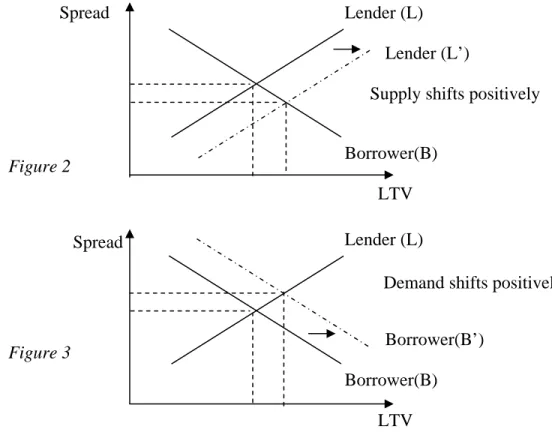
characteristics. Intuitively, lower LTV ratio provides the most direct protection to debt investors and should be associated with lower spread. However, according to previous research result, LTV ratio is an endogenous choice which is determined after negotiation between the borrower and the lender. It is likely that lenders require lower LTV ratios for borrowers or properties that generate riskier cash flows, which can attenuate or even reverse the positive relation between spreads and LTV ratios. We use a graph (Figure 1) to interpret how this mechanism of lender-borrower negotiation works.
Figure 1
The vertical axis of the graph shows the loan spread. The horizontal axis shows the
corresponding LTV ratio. From lender’s perspective, the higher the spread is, the larger amount of loan, which can be translated into higher LTV ratio, the lender is willing to supply. Moreover, the lender requires a higher spread for a higher LTV ratio given that the higher LTV ratio
represents higher risk. Hence, the curve for lender slopes upward. Holding other things equal, borrowers are usually ready to demand larger amount of loan if the price is lower. From
Spread
LTV Borrower Lender
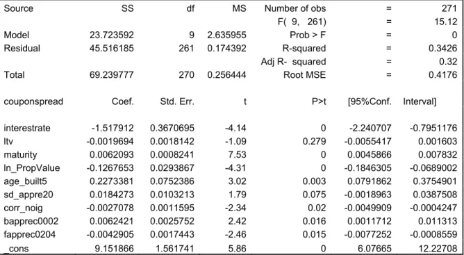
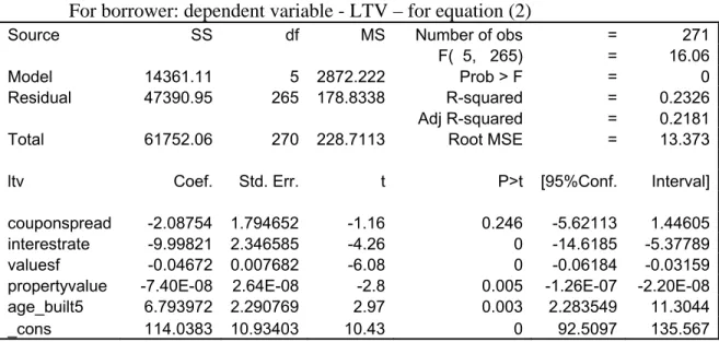
borrower’s perspective, the lower the spread is, the higher the LTV ratio is demanded. Moreover, when LTV ratio is higher, the higher risk of distress makes borrower willing to borrow only if the spread is lower. The curve for borrower is downward sloping. The closing spread and LTV ratio, at which the curves for lender and for borrower intersect, are the result of negotiation between lender and borrower. The curves represent how the demand and supply for loan depend on spread, given the certain conditions. Movement along curves depicts how much loan (LTV ratio) would be supplied and demanded given a particular spread level on the vertical axis. If conditions change, curves shift. As shown in Figure 2, if loan supply changes positively, the curve for lender shift to right from L to L’, resulting in higher LTV ratio and lower spread; likewise, in Figure 3, if loan demand changes positively, the curve for borrower shift to right from B to B’, leading to higher LTV ratio and higher spread. Using this mechanism, we can interpret the various impacts of certain conditions on the loan spread and LTV ratio.
Figure 2 Figure 3 Spread Borrower(B’) LTV Borrower(B) Lender (L)
Demand shifts positively Spread
LTV Borrower(B) Lender (L)
Lender (L’)
According to analysis above, the equation for lender describes the spread as a function of LTV ratio and the equation for borrower describes LTV ratio as a function of spread. We assume the curve for borrower, namely loan demand, is mainly determined by capital market characteristics and property characteristics while the curve for lender, that is loan supply, is determined by mortgage characteristics, capital market characteristics, property market volatility and property market correlation with nationwide market. Regarding historic and future property market growth, we think they are likely to shift either loan supply or loan demand. Therefore, two sets of structural models are used for analysis.
If property market growth shifts loan supply, we have equation (1) and (2):
For lender:
Spread = a + b* LTV ratio +c* treasury rate
+ d* maturity + ∑ei* (all property market characteristics) (1)
For borrower:
LTV ratio = f + g* spread +h* treasury rate
+ ∑ii * (property characteristics) (2)
If property market growth is put on the loan demand side, we have equation (1)’ and (2)’:
For lender:
+ n* property market volatility
+ o * correlation between sub market and nationwide property market growth (1)’
For borrower:
LTV ratio = p + q* spread + r* treasury rate + ∑si * (property characteristics)
+ t* historic property market growth + u* future property market growth (2)’
Regressions are performed at the individual loan level, but separately by property types including office, industrial, retail and apartment. Within each property type property market characteristics will apply to all loans equally whose underlying properties are in that market.
However, given that spread and LTV ratio are jointly determined, they are endogenous variables in equation (1) and (2), and hence one variable should not be included in the equation for the other without instrumental variables. Here, we take two approaches to solve this problem.
In one option, joint OLS (ordinary least square) regressions are run for spread and LTV ratio as “reduced form” outcomes of lender-borrower negotiations as followings. In equation (3), capital market and property characteristics are used as instrumental variables for LTV ratio; in equation (4), capital market, mortgage and property market characteristics are used as instrumental variables for spread.
Spread = v+ w* treasury rate +∑xi * (property characteristics)
LTV ratio = v’ + w’* treasury rate + ∑x’i * (property characteristics)
+ y’* maturity + ∑z’i* (all property market characteristics) (4)
The first option, however, does not directly present the relation between spread and LTV ratio and the mechanism of loan supply and demand. Alternatively, we use the method of 2SLS (two stage least squares) to establish the linkage. The first step is to predict loan spread and LTV ratio from Equation (3) and (4) respectively. In the second step, we use estimated LTV ratio and spread as instrumental variable for LTV ratio and spread respectively in the regressions.
Likewise, we have two sets of models separately for property market growth shifting demand or supply.
If property market growth shifts loan supply, we have equation (5) and (6):
For lender:
Spread = a’ + b’* estimated LTV ratio +c’* treasury rate
+ d’* maturity + ∑e’i* (all property market characteristics) (5)
For borrower:
LTV ratio = f’ + g’* estimated spread +h’* treasury rate
+ ∑ i’i * (property characteristics) (6)
For lender:
Spread = j’ + k’* estimated LTV ratio +l’* treasury rate + m’* maturity + n’* property market volatility
+ o’* correlation between sub market and nationwide property market growth (5)’
For borrower:
LTV ratio = p’ + q’* estimated spread + r’* treasury rate + ∑s’i * (property characteristics)
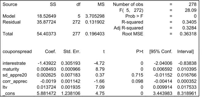
4. Description of Variables
Mortgage spread
Spread is the difference between the mortgage rate and the rate on treasury bonds with the maturity as the mortgage. Due to various maturities of mortgages, some of which are not exactly matched with maturity of treasuries, for simplicity, we use 10-year Treasury in spread calculations which has the same maturity with over 75% of loans in our data set. The error incurred by terms other than 10 year will be captured by maturity, an independent variable. Additionally, given the fact that loans typically price before closing, the spread we use as
dependent variable equals the loan coupon minus the 10-year Treasury for the month prior to the origination date.
LTV ratio
The LTV ratio is measured as the loan amount divided by the value of the property.
Capital Market Characteristic - Treasury rate
As discussed earlier, we use 10-year treasury rate for the month prior to the origination date to represent capital market characteristic in the regressions.
Mortgage Characteristic - Maturity
Maturity, namely loan term, varies from 48 months to 240 months in our data set, among which 120-month loans are over 75%.
Property Characteristic – Size effect
We use property value (or the logarithm of property value), property size (square feet) or value per square feet to capture size effect and later choose the one which is the most statistically significant as independent variable in regressions.
Property Characteristic - Building age
Building age is defined as age of property being built or age of property being renovated. In addition, because we expect that property age may not affect spread linearly, we use dummy variables for less than 5 years old and more than 5 years old. Among them, the one which is the most statistically significant will be chosen as independent variable in regressions.
Property characteristic – Property type
Each prime property type can be divided into several sub types. For example, retail includes anchored retail, single tenant retail, etc. We expect different sub type has various impact on spread. Therefore, we introduce dummy variables that characterize those sub types in regressions.
Property market risk characteristic - Property market volatility
Property market volatility is an inherent feature of property market and measured as standard deviation of change in each market’s property value or NOI (net operating income) from 1993 to 2006.
Property market risk characteristic - Correlation between sub property market and nationwide property market
Correlation is also an inherent feature of sub-market and measured as correlation of NOI growth or value appreciation between each property market and nationwide property market from 1993 to 2006.
Property market risk characteristic - Historic property market change and future property market change
Regarding property market change, we will test different spans. For example, for 2-year span, historic (backward) market change is from 2000 to 2002; future (forward) property market change is from 2002 to 2004.
Due to close relation between value and NOI, we expect their impacts on spread will offset each other. Therefore, for each of the property market risk characteristics we discussed above, we use the more statistically significant of value or NOI in regressions.
5. Data Overview
The commercial mortgage loan data for studying the relationship between loan spread and
property and mortgage characteristics is extracted from the Trepp CMBS Data Feed as of the end of 2005, provided by the Moody’s Investors Service. The original data feed includes 16 CMBS deal types: agency CMBS, agency pool, Canada, CDO, credit tenant loan, FHA, franchise loan, private loan, ReREMIC, seasoned loan, small loan, large loan, miscellaneous loan, healthcare loan, conduit loan, short term loan and single asset loan. The Trepp data feed covers all the major property types in most of the MSA markets.
The property market effect on loan spread is studied by using the TWR ISS data set – Property Price Index and Property Income Index. The data is populated over all major MSA markets and property types.
The property types and MSA markets are manually matched between the two data sets. The research data is focused on four property types: multi-family, office, industry and retail. Other property types that have either small data feed or overwhelming individuality and can not represent the main market trend are taken out of the data set. The student housing, mobile home and assistant living in the multifamily group are also stripped off.
The deal types are screened to separate the loans with direct exposure to the property and capital market risk from loans driven by factors beside market. The agency CMBS, agency pool,
Canadian loan, CDO, credit tenant loan, FHA, franchise loan, private loan, ReREMIC, seasoned loan and healthcare loan are taken out for this reason.
Blanket mortgage, pari passu deals and collateralized loans are other outliers eliminated from the data set.
Collateralized loans have pool of properties serving pool of loans. The properties can be in different MSA markets and different type. Different property type in different market carries different risks, and the correlation in between the risks makes the combination risk for such loan hard to be quantified using the available data for this research.
The pari passu loans are loans splited across multiple securitizations. In many cases, the LTV represents an abnormally low ratio, which does not reflect the real risk carried by the loan or the property. Trepp data considers equal risk for each unit or square footage, hence, derives the loan balance through square footage or unit covered by the loan. The risk premium of pari passu loan is not only driven by the market and property factors, the multiple securitizations also could have impacts on each other and skew the market effects, hence they are taken out from the data set.
Blanket mortgage is multiple loans on one property, and meanwhile, each one loan covers multiple properties. The LTV for such loans are normally nulls in the data set. Same as the other outlier loans, the interaction in between multiple loans and multiple properties complicates the risk measured by market and property characteristics. Therefore, they are eliminated from the data set for this study.
Floating rate loans are adjustable rate mortgages. The loan coupon rates are adjusted based on the current index rate. Many of the floating rate loans are in the short term or large CMBS loans, and also floating rate CMBS deals. Those are taken out from the data set.
The study truncates the time period of loans originated between the 4th quarter of 2002 and the 1st quarter of 2003, total 1083 loans in 4 property types: multifamily, office, retail and industry.
In the TWR ISS data set – Property Price Index and Property Income Index, we truncates the time period of 1993 to 2006 to study the property market volatility and the correlation between submarket and national market. Historical market change and future market change each span over two year period from 2000 to 2002 and 2002 to 2004 respectively.
6. Empirical Results
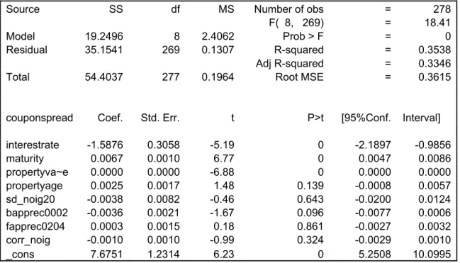
According to previous research, we include all characteristics in the regression where spread is dependent variable as shown in Exhibit 1. In theory, we expect mortgages with higher LTV ratio are associated with higher spread. However, the coefficients of LTV ratio presents both positive and negative signs for different property type and are statistically insignificant in multifamily and industry property types, which testifies the endogenous character of LTV ratio.
Exhibit 1: dependent variable-spread (including all characteristics as independent variables)
Exhibit 2 – Exhibit 7 show the regression results of equation (1) - (6) where property market growth is put on loan supply side. We’ll analyze them first.
Same as Exhibit 1, the coefficients of LTV ratio in equation (1) and loan spread in equation (2) present no consistent result, which further validates the endogenous relationship between LTV ratio and spread.
Exhibit 2: for lender: dependent variable-spread – for equation (1)
In order to deal with the endogenous factor, we use the reduced forms for spread and LTV ratio. The results of estimating regression Equation (3) and (4) are shown in Exhibit 4 and Exhibit 5 respectively. Because the results for each property type are very similar, they are discussed together.
Exhibit 4: Reduced form: dependent variable- spread – for Equation (3)
The coefficients of treasury rate in Exhibit 4 are all negative and significant but varying among the property types in Exhibit 5, indicating that treasury rate has strong negative correlation with spread but uncertain impacts on LTV ratio.
Except industrial property in Exhibit 4, coefficients for maturities are very significant for both loan spread and LTV ratio. The coefficients have consistent signs in all property types. Evidently, Mortgages with longer maturity have higher spread and lower LTV ratio.
The property value, the logarithm of property value, or value per square feet corresponding to property size effect present a strong negative correlation with spread and LTV, which reveals that economies of scale lead to lower spread and lower LTV ratio for bigger properties.
The results of regressions also reveal that brand new properties built within five years are
associated with higher spread and higher LTV ratio than properties with age more than five years. Interestingly, it seems that the renovated age doesn’t have much impact on spread or LTV ratio.
Regarding dummy variables corresponding to different sub property types, we only find they are statistically significant in explaining the LTV ratio of retail property. As shown in Exhibit 5, anchored retail has the highest spread and unanchored retail the lowest. These results indicate that lender would like to offer higher LTV to less riskier properties like anchored retail, which further inform the endogenous character of LTV ratio.
The coefficients of property market volatility (standard deviation of market growth) are insignificant and show both negative and positive signs across different property types, indicating mortgage pricing is inefficient in reflecting market volatility.
As shown in Exhibit 4, the coefficients for correlation between sub-market and nationwide property market have negative signs, though it is significant only for multifamily. This may provide some support for the negative relationship between spread and correlation.
Regarding historic market growth and future market growth, we do not find any close correlation with loan spread. Except multifamily, the coefficients for other property types are insignificant as evidenced in Exhibit 1. Although the loan spread of multifamily presents positive correlation with historic market growth and negative correlation with future market growth, the significant relationships are only found in the span of 2 year period from 2000 to 2002 and from 2002 to 2004. In addition, it should be noted that when replacing value change with NOI change in regressions, the results are even less convincing.
From the reduced forms, we do not detect any property market risks embedded in loan spread. In order to reach a firm conclusion, build a direct relation between spread and LTV ratio and interpret mechanism of loan demand and supply, alternatively we use the method of two stage least squares to treat the endogenous character of LTV ratio. The first stage is to obtain the predicted spread and LTV ratio from equation (3) and (4) as estimated by Exhibit (4) and (5).
The second stage is to use predicted spread and LTV ratio as instrumental variables for spread and LTV respectively in equation (5) and (6).
Exhibit 6: For lender: dependent variable – spread (using predicted LTV ratio from Exhibit 5 as independent variable) – for Equation (5)
Exhibit 7: For borrower: dependent variable – LTV ratio (using predicted spread from Exhibit 4 as independent variable) – for Equation (6)
In the equation for lender as shown in Exhibit 6, the coefficients of predicted LTV ratio are positive, indicating higher LTV is associated with higher spread. In the equation for borrower which determines the demand as shown in Exhibit 7, the coefficients for predicted spread are negative in all property types except industrial, indicating when spread goes up borrower will borrow less. The results of multifamily, retail and office are consistent with the supply-demand diagram we introduced in previous section. However, it should be noted that in loan demand equation the coefficient of estimated spread for industrial property is insignificant and presents different sign from other three property types.
In addition, except treasury rate and property market characteristics, other variables reinforce the results from reduced forms in equation (3) and (4). Treasury rate presents same moving
directions across different property types for lender. As shown in Exhibit 6, when treasury rate goes up, lender requires lower spread. But in the equation for borrower, treasury rate of
industrial property has different signs from others. As shown in Exhibit 7, when treasury rate goes up, borrower demands less amount of loan, i.e. lower LTV ratio for multifamily, retail and office while industrial property presents opposite variation direction. Regarding property market characteristics, the most significant results present in multifamily, and the loan spread of
multifamily shows positive relation with historic market growth and negative relation with future market growth, which is consistent with the results of equation (3).
Exhibit 8 -11 show the regression results when property market growth is put on loan demand side. The results are similar to those when property market growth drives supply. However, interestingly, in equation for borrower, the coefficients of both estimated spread and treasury rate
have negative signs across all property types including industry property, which seems to indicate that the models that put property market growth in demand side work better. We’ll further discuss it in the following section.
Exhibit 8: for lender: dependent variable-spread – for equation (1)’
Exhibit 10: For lender: dependent variable – spread (using predicted LTV ratio from Exhibit 5 as independent variable) – for Equation (5)’
Exhibit 11: For borrower: dependent variable – LTV ratio (using predicted spread from Exhibit 4 as independent variable) – for Equation (6)’
7. Interpretation of Results
In order to understand the underneath economical mechanism of the regression results, we use the loan demand-supply equilibrium graphs introduced in methodology section to interpret them.
Capital Market Characteristic - Treasury rate
Figure 4
Spread is the premium over Treasury rate the lender requires for bearing risks. Treasury rate drives both demand and supply. As risk-free rate, when treasury rate goes up, the lender may need some time to make reaction and hence accept lower spread which still results in same or higher total return while the borrower will decrease loan demand for a given level of spread due to higher borrowing cost. The results of equation (5), equation (6) excluding industrial property, equation (5)’and equation (6)’ as shown in Exhibit 6, 7, 10 and 11 validate this impact of
treasury rate on lender and borrower. As a result, the curve for lender shifts to the right from L1 to L2 while the curve for borrower shifts to the left from B1 to B2. As shown in figure 4, higher treasury rate leads to lower spread and uncertain LTV ratio which could be higher, lower or
Treasury rate increases
LTV Borrower(B2) Borrower(B1) Spread Lender(L1) Lender(L2)
stable, which is consistent with the regression results of equation (3) and (4) as shown in Exhibit 4 and 5.
Mortgage Characteristic - Maturity
Figure 5
As maturity lengthens, for a given level of LTV ratio the lender requires higher spread to
compensate the higher risk derived from longer payback period. As a result, the curve for lender shifts to the left from L1 to L3. As shown in figure 5, higher maturity leads to higher spread and lower LTV ratio, which is consistent with the regression results.
Property Characteristic – Size effect
Larger properties are usually held by large institutions including pension funds, REITs, foreign investment institutions, etc. Such large institutions often have “deep pockets”, that is, lots of cash that they need to invest as equity, and they also often tend to have a more conservative investment philosophy than the less-bureaucratic and more entrepreneurial smaller investors. The result would be that larger properties, as purchased primarily by large institutions, would have more equity (less debt) in their capital structure. Moreover, large institutions tend to be either
Borrower(B1) Spread Lender (L1) Maturity increases LTV Lender (L3)
tax-exempt, or to have multiple investor/owner/partners who face varying tax situations. This dilutes the incentive large real estate investment institutions have for maximizing income tax savings. Comparatively, income tax shield benefits are more of a motivation for the smaller, local investors than for the larger institutions. In addition, the smaller, more entrepreneurial and more local investors who tend to dominate more in the small property purchases also often have a type of information advantage. They are expert in their own local real estate market where they are investing. This information advantage may give them extra confidence that they know the risks, which makes them less afraid to lever to the maximum. Lastly, investors in the CMBS market penalize large, lumpy deals, which can result from some large loans. The unevenness of the risk profile of a lumpy deal can be inconsistent with size of the tranch, particularly for anything other than Aaa, and can reduce liquidity. Furthermore, a deal with a few very large loans will also have a low Herf measure and therefore be penalized in subordination levels. As a result, large loans tend to be more conservatively leveraged in order to offset that aversion to lumpiness. In fact, the very definition of a "fusion" deal is: the combination of a large number of small loans (aka conduit loans) and a small number of large loans with low leverage. This trend was exacerbated after 9/11 which consciousness of the importance of large loans in a deal was highlighted. Figure 6 Borrower(B3) Size increases LTV Borrower(B1) Spread Lender
Therefore, borrower with bigger property demands less amount of loan for a certain spread. As a result of bigger property, the curve for borrower shifts to the left from B1 to B3. It can be seen from figure 6 that bigger property leads to lower spread and lower LTV ratio. The results of regressions also reveal the significant negative relation between property size effect and the spread and LTV ratio.
Property Characteristic - Building age
Figure 7
Borrowers with brand new properties expect income growth as properties come to stabilization and mature management, and therefore can accept a higher spread for a certain LTV ratio than borrowers with older properties. With unstable cash in flow, the new property often requires higher leverage comparing to the stable properties. As a result, when property is newer, the curve for borrower shifts to the right from B1 to B4. As shown in figure 7, newer property has higher spread and higher LTV ratio. This is consistent with the results of regressions which reveal that new properties built within five years are associated with higher spread and higher LTV ratio than properties with age more than five years.
Borrower(B4) Newer property LTV Borrower(B1) Spread Lender Borrower(B4) Newer property LTV Borrower(B1) Spread
Property Market Risk Characteristic - Property market volatility
Figure 8
As market volatility increases, given a certain LTV ratio, lender would require higher spread due to the increase in default risk. Consequently, when market becomes more volatile, the curve for lender shifts to left from L1 to L4. As shown in figure 8, higher market volatility leads to higher spread and lower LTV ratio. However, in regression results, coefficients for market volatility present different signs and mostly are insignificant for each property type, suggesting that mortgage pricing is inefficient in reflecting property market volatility.
Property Market Risk Characteristic - Correlation between sub property market and nationwide property market
Figure 9
As correlation increases, given a certain LTV ratio, lender would require lower spread because operating in line with national property market makes property market risks more predictable
Volatility increases LTV Borrower(B1) Spread Lender (L1) Lender (L4) Borrower(B1) Lender (L1) Lender (L5) Correlation increases LTV Spread
and controllable. As a result, when market correlation with total property market increases, the curve for lender shifts to the right from L1 to L5, which leads to lower spread and uncertain LTV ratio as shown in figure 9. However, the regression results show that the coefficients for
correlation between sub-market and nationwide property market are insignificant except in reduced form for spread of multifamily. Although in lender’s equations the coefficients for correlation have negative signs, this doesn’t provide enough support for mortgage pricing efficiency in reflecting market correlation.
Property Market Risk Characteristic - Historic property market change and future property market change
In theory, the position in the real estate cycle decides the price of risk. The peak of the market indicates the future trough, while the bottom of the market predicts the up going trend in the future. When market booms, as represented by point A in figure 10, lenders expect that the market will go down and hence require higher spread. This mechanism is illustrated in Figure 11. When property market goes up to the peak, the curve for lender shifts to the left from L1 to L6, which leads to higher spread and lower LTV ratio. On the contrary, when market is at the bottom, as represented by point B in Figure 8, lenders predict market will go up and hence require lower spread. As shown in Figure 12, when property market goes down to bottom, the curve for lender shifts to the right from L1 to L7, which leads to lower spread and higher LTV ratio. Finally, holding other things equal, we expect the highest spread at the peak of market and lowest spread at the bottom of market. Figure 10 shows that loan spread is positively related to previous market growth and reversely related to future market growth.
Figure 10
Figure 11
Figure 12
The regression results as discussed in previous section show that the coefficients of backward-forward market growth variables are significant only in the reduced form for spread of
multifamily (see Exhibit 4), where spread presents positive correlation with backward market growth and negative correlation with forward market growth. However, the coefficients of these
B - minimum spread A - maximum spread
Property market goes up to the peak
LTV Borrower(B1) Spread Lender (L1) Lender (L6) Borrower(B1) Lender (L1) Lender (L7)
Property market goes down to the bottom
LTV Spread
variables in reduced form for LTV ratio of multifamily (see Exhibit 5) are insignificant and have the same signs as in Exhibit 4. This seems to imply that spread and LTV ratio are highest at the market peak and lowest at the bottom, which is inconsistent with the theoretical interpretation we discussed above.
Since there is little evidence that the market cycle shifts lender supply, we would explain the results as that borrower demand is strongest at the peak of market and lowest at the trough. As shown in Figure 13 and 14, when market goes to peak or bottom, loan demand, namely the curve for borrower shifts, suggesting that spread and LTV ratio is highest at the market peak and lowest at the bottom, which is consistent with the results of reduced form for multifamily.
Figure 13
Figure 14
Borrower(B5)
Property market goes down to the bottom
LTV Borrower(B1) Spread Lender Lender Borrower(B4)
Property market goes down to the peak
LTV Borrower(B6) Spread
The Exhibit 8-11 estimated by equation (1)’, (2)’, (5)’ and (6)’ present the results of putting property market growth on the demand side. As we analyzed in previous section, this set of models gets the same signs for treasury rate and predicted spread in borrower’s equation across all property types, which indicates this set of models works better and hence provides some evidence that property market growth drives demand not supply. However, we still can’t find systematic impact of property market characteristics on spread and LTV ratio across all property types.
8. Conclusion
MSA property market is a major factor in credit performance of the loans in CMBS and in the securities themselves. If mortgage pricing is efficient, it should capture property market variation risk and inherent risk. The thesis takes a rigorous quantitative approach to test the relationship between commercial mortgage pricing and property market risk.
Providing lenders with the most direct protection, LTV ratio is supposed to be the most important determinants of mortgage pricing and should have significant positive impacts on spread. However, empirical results show that LTV ratio is an endogenous choice which is
determined after negotiations between lender and borrower. The reduced form and 2SLS method are used to deal with the endogenous factor. Meanwhile, we use a loan demand-supply diagram to interpret how various determinants influence loan spread and LTV ratio. This makes a big improvement over understanding the relationship between LTV ratio and mortgage spread.
The mortgage demand-supply diagram interprets the dynamic relationship between loan spread and property characteristics, mortgage loan characteristics, property market characteristics and capital market characteristics. Property characteristics, represented by property size effect and age, drive the loan demand. Larger property size and older age drive down the loan demand, hence lead to lower spread. Mortgage characteristics, represented by maturity drive loan supply schedule. Longer maturity is associated with higher spread and lower LTV ratio. Treasury rate, as one of capital market characteristics, drives both the loan demand and supply. Higher treasury
rate leads to lower spread and uncertain LTV ratio. However, property market characteristics appear to play little, if any, role in shifting either the loan demand or supply schedule. This indicates that property market risk characteristics have little systematic impact on spread and LTV ratio across property types. It should be noted that some evidence was found showing that backward and forward market growth shift loan demand in multifamily property type, but no evidence of such shift in loan supply. But our test still shows no commanding roles of property market risks in determining loan pricing.
In conclusion, there is little linkage between property market risk and original loan spread. We may say that commercial mortgage is mispriced in terms of property market risk.
Due to the limited data base of the thesis, we only use the six month mortgage data from October 2002 to March 2003 in analysis. Going forward, future research can be extended to longer or more recent period to achieve a more generalized analysis of commercial loan pricing.
Bibliography
B. Ambrose & A. B. Sanders (2003), "Commercial Mortgage (CMBS) Default and Prepayment Analysis", Journal of Real Estate Finance and Economics, Vol. 26, No. 2-3, March-May 2003 B. A. Maris & W. Segal (2002), “Analysis of Yield Spreads on Commercial Mortgage-Backed Securities”, Journal of Real Estate Research, Vol. 23, No. 03, May/June 2002, 235-252
Campbell, J.Y. and Shiller R. J., (2001), “Valuation Ratios and The Long-Run Stock Market Outlook: an Update”, Working Paper 8221, http://www.nber.org/papers/w8221
Frank E. Nothaft and James L. Freund (2003), “The Evolution of Securitization in Multifamily Mortgage markets and Its Effect on lending Rates”, Journal of Real Estate Research, Vol. 25, No. 02, Apr-Jun.2003, 91-112
Grissom, T., D. Hartzell and C. Liu, (1987). “An Approach to Industrial Real Estate Markets Segmentation and Valuation Using the Arbitrage Pricing Paradigm”, Real Estate Economics 15, 199-218
Lusht, K.M. and Fisher, J.D. (1984), “Anticipated Growth and the Specification of Debt in Real Estate Value Models”, Real Estate Economics, Volume 12, Number 1, March 1984, pp. 1-11(11) P.H. Hendershott and B. Turner (1999), “Estimating Constant-Quality Capitalization Rates and Capitalization Effects of Below Market Financing”, Journal of Property Research 16: 109-122 Ping Cheng (2005), “Asymmetric Risk Measures and Real Estate Returns”, The Journal Of Real Estate Finance and Economics, 30:1, 89-102, 2005
P. Sivitanides, J. Southard, R.G. Torto, W. Wheaton (2001), “The Determinants of Appraisal-Based Capitalization Rates”, Real Estate Finance, Summer, 2001, Page 1
R. Sivitanidou and P. Sivitanidies (1999), “Office Capitalization Rates: Real Estate and Capital Market Influences”, Journal of Real Estate Finance and Economics, 18, 297-322
Shilling, James D . (2003), “Is There a Risk Premium Puzzle in Real Estate?”, Real Estate Economics, Bloomington: Winter 2003. Vol.31, Iss. 4; pg. 501, 25 pgs
S. Gordon & L. Kizer (2006), “US CMBS: The Missing Link Between Commercial Mortgage Loan Spreads and Property Market Risk”, Moodys Special Report
Sivitanides, P. S. (1998), “A Downside-risk Approach to Real Estate Portfolio Structuring”, Journal of Real Estate Portfolio Management 4, 159-168
Sing, T. F. and Ong, S. E. (2000), “Asset Allocation in a Downside Risk Framework”, Journal of Real Estate Portfolio Management 6, 213-224
Titman, Sheridan, Tompaidis, Stathis and Tsyplakov, Sergey (2005), “Determinants of Credit Spreads in Commercial Mortgages”, Real Estate Economics, Volume 33, Number 4, December 2005, pp. 711-738(28)
Appendix
Table 1: Multifamily
dependent variable - spread (including all characteristics as independent variables)
Source SS df MS Number of obs = 271
F( 9, 261) = 15.12
Model 23.723592 9 2.635955 Prob > F = 0
Residual 45.516185 261 0.174392 R-squared = 0.3426
Adj R- squared = 0.32
Total 69.239777 270 0.256444 Root MSE = 0.4176
couponspread Coef. Std. Err. t P>t [95%Conf. Interval]
interestrate -1.517912 0.3670695 -4.14 0 -2.240707 -0.7951176 ltv -0.0019694 0.0018142 -1.09 0.279 -0.0055417 0.001603 maturity 0.0062093 0.0008241 7.53 0 0.0045866 0.007832 ln_PropValue -0.1267653 0.0293867 -4.31 0 -0.1846305 -0.0689002 age_built5 0.2273381 0.0752386 3.02 0.003 0.0791862 0.3754901 sd_appre20 0.0184273 0.0103213 1.79 0.075 -0.0018963 0.0387508 corr_noig -0.0027078 0.0011595 -2.34 0.02 -0.0049909 -0.0004247 bapprec0002 0.0062421 0.0025752 2.42 0.016 0.0011712 0.011313 fapprec0204 -0.0042905 0.0017443 -2.46 0.015 -0.0077252 -0.0008559 _cons 9.151866 1.561741 5.86 0 6.07665 12.22708 Table 2: Multifamily
For lender: dependent variable-spread – for equation (1)
Source SS df MS Number of obs = 271
F( 7, 263) = 15.21
Model 19.94886 7 2.849837 Prob > F = 0
Residual 49.29092 263 0.187418 R-squared = 0.2881
Adj R-squared = 0.2692
Total 69.23978 270 0.256444 Root MSE = 0.43292
couponspread Coef. Std. Err. t P>t [95%Conf. Interval] interestrate -1.51858 0.379267 -4 0 -2.26537 -0.77179 ltv -0.00063 0.001855 -0.34 0.733 -0.00428 0.003018 maturity 0.007075 0.000832 8.5 0 0.005436 0.008714 sd_appre20 0.016786 0.010687 1.57 0.117 -0.00426 0.037829 corr_noig -0.00173 0.001182 -1.47 0.144 -0.00406 0.000596 bapprec0002 0.006352 0.002628 2.42 0.016 0.001178 0.011526 fapprec0204 -0.00424 0.001777 -2.39 0.018 -0.00774 -0.00074 _cons 6.959851 1.542148 4.51 0 3.923323 9.996379
Table 3: Multifamily
For borrower: dependent variable - LTV – for equation (2)
Source SS df MS Number of obs = 271
F( 5, 265) = 16.06
Model 14361.11 5 2872.222 Prob > F = 0
Residual 47390.95 265 178.8338 R-squared = 0.2326
Adj R-squared = 0.2181
Total 61752.06 270 228.7113 Root MSE = 13.373
ltv Coef. Std. Err. t P>t [95%Conf. Interval]
couponspread -2.08754 1.794652 -1.16 0.246 -5.62113 1.44605 interestrate -9.99821 2.346585 -4.26 0 -14.6185 -5.37789
valuesf -0.04672 0.007682 -6.08 0 -0.06184 -0.03159
propertyvalue -7.40E-08 2.64E-08 -2.8 0.005 -1.26E-07 -2.20E-08 age_built5 6.793972 2.290769 2.97 0.003 2.283549 11.3044
_cons 114.0383 10.93403 10.43 0 92.5097 135.567
Table 4: Multifamily
Reduced form: dependent variable- spread – for Equation (3)
Source SS df MS Number of obs = 271
F( 8, 262) = 16.85
Model 23.51809 8 2.939761 Prob > F = 0
Residual 45.72169 262 0.174510 R-squared = 0.3397
Adj R-squared = 0.3195
Total 69.23978 270 0.256444 Root MSE = 0.41774
couponspread Coef. Std. Err. t P>t [95%Conf. Interval]
interestrate -1.47149 0.36469 -4.03 0 -2.18959 -0.75338 maturity 0.00645 0.00080 8.11 0 0.00488 0.00801 ln_PropValue -0.12270 0.02916 -4.21 0 -0.18011 -0.06529 age_built5 0.21574 0.07450 2.9 0.004 0.06904 0.36243 sd_appre20 0.01772 0.01030 1.72 0.087 -0.00257 0.03801 corr_noig -0.00261 0.00116 -2.26 0.025 -0.00489 -0.00034 bapprec0002 0.00628 0.00258 2.44 0.015 0.00121 0.01135 fapprec0204 -0.00391 0.00171 -2.29 0.023 -0.00727 -0.00054 _cons 8.74070 1.51563 5.77 0 5.75634 11.72507
Table 5: Multifamily
Reduced form: dependent variable- LTV ratio – for Equation (4)
Source SS df MS Number of obs = 271
F( 8, 262) = 9.69
Model 14094.867 8 1761.8584 Prob > F = 0
Residual 47657.194 262 181.8977 R-squared = 0.2282
Adj R-squared = 0.2047
Total 61752.061 270 228.7113 Root MSE = 13.487
ltv Coef. Std. Err. t P>t [95%Conf. Interval]
interestrate -20.2670 11.7868 -1.72 0.087 -43.4759 2.9419 maturity -0.0992 0.0253 -3.92 0 -0.1490 -0.0494 valuesf -0.0496 0.0085 -5.84 0 -0.0663 -0.0328 age_built5 7.0304 2.3386 3.01 0.003 2.4254 11.6353 sd_appre20 0.1105 0.3352 0.33 0.742 -0.5495 0.7705 corr_noig -0.0397 0.0369 -1.08 0.282 -0.1123 0.0329 bapprec0002 0.0839 0.0844 0.99 0.321 -0.0823 0.2500 fapprec0204 -0.0923 0.0582 -1.59 0.114 -0.2070 0.0224 _cons 164.1503 47.1231 3.48 0.001 71.3621 256.9385 Table 6: Multifamily
For lender: dependent variable – spread
(using predicted LTV ratio from Table 5 as independent variable) – for Equation (5)
Source SS df MS Number of obs = 271
F( 7, 263) = 15.43
Model 20.16084 7 2.88012 Prob > F = 0
Residual 49.07894 263 0.186612 R-squared = 0.2912
Adj R-squared = 0.2723
Total 69.23978 270 0.256444 Root MSE = 0.43199
couponspre~1 Coef. Std. Err. t P>t [95% Conf. Interval]
interestra~1 -1.36704 0.395313 -3.46 0.001 -2.14542 -0.58866 maturity 0.007766 0.000981 7.92 0 0.005836 0.009697 sd_appre20 0.014681 0.010781 1.36 0.174 -0.00655 0.03591 corr_noig -0.00153 0.001189 -1.29 0.198 -0.00388 0.000806 bapprec0002 0.006558 0.002627 2.5 0.013 0.001386 0.01173 fapprec0204 -0.00301 0.002 -1.51 0.133 -0.00695 0.000924 p_ltv 0.005848 0.005224 1.12 0.264 -0.00444 0.016134 _cons 5.83005 1.75876 3.31 0.001 2.367007 9.293093
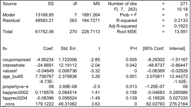
Table 7: Multifamily
For borrower: dependent variable – LTV ratio
(using predicted spread from Table 4 as independent variable) – for Equation (6)
Source SS df MS Number of obs = 271
F( 5, 265) = 14.96
Model 13595.66 5 2719.131 Prob > F = 0
Residual 48156.4 265 181.7223 R-squared = 0.2202
Adj R-squared = 0.2055
Total 61752.06 270 228.7113 Root MSE = 13.48
ltv Coef. Std. Err. t P>t [95% Conf. Interval]
interestra~1 -33.5486 12.80673 -2.62 0.009 -58.7645 -8.33269 p_spread_f -11.4176 3.235647 -3.53 0 -17.7884 -5.04674 valuesf -0.04751 0.007737 -6.14 0 -0.06275 -0.03228 age_built5 8.202722 2.34916 3.49 0.001 3.577328 12.82812 propertyva~e -8.79E-08 2.76E-08 -3.19 0.002 -1.42E-07 -3.36E-08
_cons 226.1252 53.62557 4.22 0 120.5388 331.7116
Table 8: Multifamily
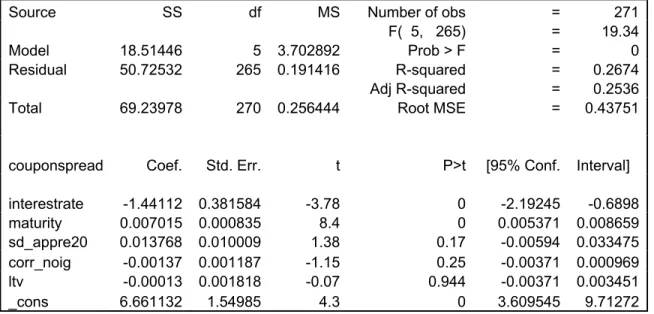
For lender: dependent variable-spread – for equation (1)’ (removing property market growth from independent variables)
Source SS df MS Number of obs = 271
F( 5, 265) = 19.34
Model 18.51446 5 3.702892 Prob > F = 0
Residual 50.72532 265 0.191416 R-squared = 0.2674
Adj R-squared = 0.2536
Total 69.23978 270 0.256444 Root MSE = 0.43751
couponspread Coef. Std. Err. t P>t [95% Conf. Interval]
interestrate -1.44112 0.381584 -3.78 0 -2.19245 -0.6898 maturity 0.007015 0.000835 8.4 0 0.005371 0.008659 sd_appre20 0.013768 0.010009 1.38 0.17 -0.00594 0.033475 corr_noig -0.00137 0.001187 -1.15 0.25 -0.00371 0.000969 ltv -0.00013 0.001818 -0.07 0.944 -0.00371 0.003451 _cons 6.661132 1.54985 4.3 0 3.609545 9.71272