HAL Id: hal-01406731
https://hal-univ-paris.archives-ouvertes.fr/hal-01406731
Submitted on 1 Dec 2016
HAL is a multi-disciplinary open access
archive for the deposit and dissemination of
sci-entific research documents, whether they are
pub-lished or not. The documents may come from
teaching and research institutions in France or
abroad, or from public or private research centers.
L’archive ouverte pluridisciplinaire HAL, est
destinée au dépôt et à la diffusion de documents
scientifiques de niveau recherche, publiés ou non,
émanant des établissements d’enseignement et de
recherche français ou étrangers, des laboratoires
publics ou privés.
and dilatancy
Christophe Coste
To cite this version:
Christophe Coste. Shearing of a confined granular layer: Tangential stress and dilatancy. Physical
Review E : Statistical, Nonlinear, and Soft Matter Physics, American Physical Society, 2004, 70,
�10.1103/PhysRevE.70.051302�. �hal-01406731�
Shearing of a confined granular layer: Tangential stress and dilatancy
C. CosteGroupe de Physique des Solides, Campus Boucicaut 140 rue de Lourmel, 75015 Paris, France
(Received 11 June 2004; published 5 November 2004)
We study the behavior of a confined granular layer under shearing, in an annular cell, at low velocity. We give evidence that the response of the granular layer under shearing is described by characteristic length scales. The tangential stress reaches its steady state on the same length scale as the dilatancy. Stop-and-go experiments performed at several driving velocities show a logarithmic increase of the static friction coefficient with waiting time, followed by rejuvenation on a characteristic length of the order of the magnitude of a Hertz contact between adjacent grains. The dilatancy does not evolve during the stop, neither during the elastic reloading when the driving is resumed. There is a small variation when sliding sets anew, which corresponds to the rejuvenation of the layer, and this variation is independent of the waiting time. We argue that aging is due to the behavior of individual contacts between grains, not global evolution of the piling. Under an instanta-neous increase of the velocity, the tangential stress reaches a new steady state, exhibiting velocity strengthening behavior. An increase of dilatancy is also observed. It is much larger than fluctuations in the steady state, variations in a stop and-go-experiment, but much less than for shearing of freshly poured grains. The dilatancy variation during a velocity jump is not due to structural rearrangements of the piling. The evolutions of tangential stress and dilatancy are logarithmic in the ratio of upper and lower velocities.
DOI: 10.1103/PhysRevE.70.051302 PACS number(s): 45.70.Mg
I. INTRODUCTION
The behavior of a sheared granular medium is important for the design of silos and hoppers used to handle and store many industrial materials[1] or for the understanding of the frictional behavior of earthquake faults[2,3]. This is also a fundamental question of granular mechanics. In this paper, we are concerned with low shear rates[see below, Eq. (1)]. Problems of interest in this regime include stick-slip insta-bilities [4,5], coupling between friction and dilatancy
[4,6–8], behavior of the granular layer at large shearing
dis-tances [9,10], shear banding and strain localization
[3,6,10–13], aging [5,12,14,15], and response to an
instanta-neous velocity jump[3,7,16]. In what follows, we will insist on the approach toward a steady state, then discuss aging under constant normal and tangential stress, and last the re-sponse to velocity jumps.
Many laboratory devices may be used to study the re-sponse of a granular layer to shear. The simplest apparatus may be a plate, placed on the top of a granular layer, driven at a controlled velocity [8,14]. The granular matter may be put into two boxes, separated by a small gap, in relative translation and under normal stress: the direct shear box[6]. Geophysicists simulate the granular matter contained in faults by inserting a granular layer(the gouge) between two granite blocks; the relative translation and normal stress are applied to those blocks [7,15]. An inconvenience of those setups is that the displacement is limited to a few centime-ters. One way to avoid this limitation is to use a Couette geometry [10,12,13]. In this geometry, experiments have been done at constant density[12,13] or under constant pres-sure by submitting the granular layer to a radial stress[10]. A third possibility is the use of an annular plane Couette geom-etry[3–5,9,16], in which the grains are contained in an an-nulus, relative motion imposed between this annulus and the cover plate, and constant pressure applied on the cover plate.
If the mean radius of the annulus is large compared to its width, we can neglect the radial velocity gradient and this setup is very similar to the direct shear box. This is the geometry used in the present study.
A peculiarity of our shearing apparatus is that the grains cannot escape from the cell, allowing unambiguous measure-ments of the layer dilatancy. When poured in the experimen-tal cell, the grains are in a dense state. The average volume fraction is 0.61% ± 1% (see below, Sec. II B), very close to the so called random close packing of 0.637 [17]. In this regime, shearing necessarily implies dilatancy of the granu-lar layer [18]. The coupling between shear stress and dila-tancy is still an open problem in granular media mechanics, about which we provide experimental information.
Our experiments are done at low driving velocity V, typi-cally V苸关3⫻10−3, 1兴 d/s in units of grain diameter d per second. More precisely, we may define a dimensionless shear rate I[19], which compares the relative importance of inertia and confining stresses. With the ⍀ angular velocity, R¯ the mean cell radius, H the cell depth,the grain density, and N the normal stress, we set
I⬅ 共⍀R¯/H兲d
冑
N/ 苸 关2 ⫻ 10−6,2⫻ 10−4兴. 共1兲
We are thus always in a very-low-shear-rate regime. In our experiments, we impose the driving velocity and normal stress to the system and measure global quantities, the average tangential stress, and the average dilatancy of the layer. We carefully compare the dynamics of those two quan-tities. We study the transient to reach a steady shearing, be-ginning with freshly poured grains, under a constant driving velocity. We then discuss stop-and-go experiments and aging and the system response to instantaneous velocity jumps.
In Sec. II, we describe our experimental configuration. Section III is devoted to the presentation and discussion of our experimental results. More specifically, we discuss steady-state shearing of freshly poured grains in Sec. III A, stop-and-go shear experiments in Sec. III B, and velocity jumps in Sec. III C. The conclusions are summarized in Sec. IV.
II. EXPERIMENTAL SETUP A. Description of the apparatus
The experimental setup is an annular cell of inner radius 103 mm, outer radius 117 mm, and depth 20 mm. It is placed on an annular rotation stage (Newport RV240PP), with a stepper motor drive. The cover plate is prevented from following the rotation by using a cantilever spring, of stiff-ness k = 2.25⫻105N / m. In order to shear the bulk of the
granular layer, the cover plate has steel teeth, 5 mm long, every 30°(see Fig. 1). With this setup, shearing occurs in the plane tangent to the teeth extremities.
The cell width 共14 mm兲 is much smaller than its mean radius R¯ 共110 mm兲, so that in the following we consider the shearing velocity V as almost uniform in width, simply re-lated to the angular velocity ⍀ by V=R¯⍀. This has been shown to be basically correct for annular cells much larger in comparison with their mean radius[5]. The angular velocity
⍀ ranges from 50⫻10−6 to 16⫻10−3rad/ s, so that the
ve-locity ranges from 5m / s to 1750m / s, that is, from 3
⫻10−3d / s to 1 d / s in units of a grain diameter d
⬇1.5 mm. The experiments are thus all done in the
low-shear-rate regime IⰆ1 [see Eq. (1)].
The cover plate is free to move vertically, and three posi-tion sensors measure its height. With those three measure-ment points, we get the mean displacemeasure-ment of the cover, hence the dilatancy of the granular layer. The cell and cover are designed in such a way that no grain can escape during
the shearing, despite a gap between the cover and annulus that prevents friction between them.
The deflection of the cantilever spring is measured by another position sensor, in order to know the mean shearing stress applied to the granular layer. Some masses may be added to the cover plate, so that the weight is in the range
关32,110兴N (which corresponds to a normal stress N between
3.30 and 11.34 kPa). The weight of the cover alone is more than 12 times that of the grains themselves.
B. Preparation of a sample
The grains are glass beads, of diameter 1.5% ± 10% mm. Before using them in an experiment, we wash them carefully in distilled water with an ultrasonic cleaner. This manipula-tion spectacularly decreases the wear during the experiments: it allows up to 15 m of cumulated sheared distance without any systematic variation on the effective friction coefficient or dilatancy. It suppresses also stick-slip oscillations during shearing.
In order to improve the reproducibility of our experi-ments, we prepare all samples in the same way. The grains are poured with the help of a hopper, maintaining a constant angular velocity of the empty cell of 20° / s. When the cell is full, the upper surface of the grain is not flat. We thus change the velocity down to 5 ° / s and drop the beads that may be in excess with the help of a rake. At the end of this process, the height of the grains layer is 20 mm± 75m, and its mass is 266± 2 g—, that is, an average volume fraction of 0.61% ± 1%. Granular media dynamics is oversensitive to small variations in density[20], and this uncertainty is most likely responsible for the scatter of the effective dynamical friction coefficient(see below section III A).
The zero of dilatancy is, in all experiments, chosen to be the position of the cell cover when we place it on the freshly poured grains. Ideally, the zero should be fixed once and for all. There are nevertheless two causes of inaccuracy. The first is that we have to remove the sensors to pull up the cell cover and empty the cell, and we cannot be sure to replace them exactly in the same fashion from one experimental run to the other. The second is that despite our care, the upper surface of the grains is not perfectly flat and not at the same mean position after each pouring process. The zero is thus known to a precision of ±75m. This value is used above to estimate the uncertainty on the depth of the granular layer.
III. EXPERIMENTAL RESULTS A. Shearing of freshly poured grains
In Fig. 2, we display the evolution of the tangential stress
T, normalized by the normal stress N(upper plot), and of the
dilatancy as a function of the displacement L (lower plot). The rotation angle is defined as the product of the driving angular velocity by the time since we start the motor. During elastic loading of the cantilever spring,does not represent a shearing angle, but rather the deformation of the spring. In what follows we are interested in much larger rotations. The linear displacement L is defined as L⬅R¯. The experiments shown in Fig. 2 are done for a normal stress of 9.73 kPa and FIG. 1. Sketch of the apparatus. The drawing on the right is an
upper view, showing the cell that contains the beads and the 12 steel teeth of the cover that are buried in them. The large arrow indicates the imposed rotation of the cell; the cover is blocked by a cantilever spring(not shown in the drawing), the deflection of which gives the tangential stress applied on the beads. The drawing on the left is a cutting of the side view. The bottom arrow indicates the imposed motion of the cell, while the top arrow indicates the motion of the cover, moving freely in the vertical direction because of the dila-tancy of the granular layer.
driving velocities respectively equal to 11, 110, and 1100m / s.
Let us first consider the evolution of the tangential stress. The initial response of the granular layer to the driving, along the first 90m, is shown in the inset. We see that the tangential stress evolves linearly with distance. Moreover, this evolution is reversible and no hysteresis is observed when we reverse the direction of rotation. This initial re-sponse is thus elastic, with a effective stiffness of 2.8
⫻105N / m, which does not depend on the velocity. Beyond
typically 150m, the response is plastic and hysteresis be-comes observable. If we continue further the motion of the annular cell, the tangential stress reaches a maximum T =sN, then decreases toward a stationary value T =dN (apart from fluctuations, which are dealt with below). The
maximumsmay be defined as a static friction coefficient.
When it has been reached, the granular layer undergoes slid-ing at a constant velocity V. The coefficientd, defined as
the average of T / N in this steady state, may indeed be iden-tified with a dynamic friction coefficientd⬍s, as for solid
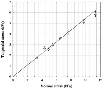
friction. When we plot the tangential stress in the steady state as a function of the normal stress, as in Fig. 3, we indeed obtain a straight line, with a sloped⬇0.54.
In the experiments shown in Fig. 2, an additional mass of 6.33 kg is placed on the cover, which explains why the initial dilatancy is negative. The evolution of dilatancy, shown in the lower curve, is typical of dense granular pilings([1], Sec. 6.5). There is first compaction (about 50m), then dilatancy of the layer up to 450m. The order of magnitude of this effect may be recovered in a very simple fashion. As a very crude approximation, suppose an initial regular HCP lattice. A bead is supported by three others, and its center is at a height R
冑
8 / 3 from the plane defined by the three beadcen-ters. The bead may slide if it increases its height up to R
冑
3, being in contact with only two of the underlying beads. Hence the dilatancy is⌬h⬇NR共冑
3 −冑
8 / 3兲, where N⬇10 is the number of beads between the teeth extremities and the cell bottom. This gives⌬h⬇750m, which is an overesti-mate since the initial experimental packing fraction of 0.61 is less than the HCP one of 0.74.The striking feature of Fig. 2 is that either the tangential stress(upper curves) or the dilatancy (lower curves) evolves in the same fashion with distance, rather independently from the velocity, which varies by two orders of magnitude. Those evolutions are characterized by typical length scales, not by time scales.
This discussion may be made more precise if we define several typical length scales for the system. First we intro-duce L共s兲, which is the distance necessary to reach the maximum of tangential stress, after the elastic loading of the granular layer. Then we may define L共d兲, as the distance necessary to reach the tangential stress steady state. In order to get a result which does not depend too much on fluctua-tions, we plot the tangent to the curve T / N, shortly after the maximum. We then define L共d兲 as the necessary distance to decrease towarddalong this tangent.
Let us now consider the evolution of the dilatancy. We define a length scale L共hmin兲 as the position of the minimum
of dilatancy. Then we introduce L共h⬁兲 as the distance neces-sary to reach the steady-state dilatancy h⬁. We take advan-tage of the fact that two straight lines naturally appear, tan-gent to the experimental curve: one during the almost linear increase of dilatancy that follows the minimum and the other almost parallel to the abcissa axis in the stationary regime. The intersection of those two straight lines provides a good definition of L共h⬁兲, quite insensitive to fluctuations.
The values of those four different length scales are listed in Table I, which shows that indeed they do not depend on FIG. 2. Plot of T / N(upper curves) and the dilatancy (inm,
lower curves) as a function of displacement (in cm), for the same normal stress共9.73 kPa兲 and several driving velocities: 11m/s 共䊊兲, 110m/s 共䊐兲, and 1100 m/s 共ⴱ兲. In the upper curve, the inset shows the very begining of the motion, when elastic response of the layer occurs. The data correspond to three different initial states of freshly poured grains. The spatial resolution(1 point per micrometer) is the same for all data, but for clarity the symbols are shown each 1000 points only. The properties of the curves are sum-marized in Table I.
FIG. 3. Plot of the tangential stress(in kPa) as a function of the normal stress (in kPa). The tangential stress is measured in the steady state, for a driving velocity of 11m/s. The error bars cor-respond to the 7% fluctuations level observed in the steady state. The slope of the straight line, which is constrained to go through the origin, is the average of all values ofd,具d典=0.54.
the driving velocity. This result is quite obvious for L共s兲. It only evidences that there is indeed a static friction coeffi-cient, which implies a sufficient deformation of the cantile-ver spring in order for sliding to begin. This length scale thus appears because of the measuring process. This explanation is not relevant for the other length scales. Their very exis-tence is strong evidence that the collective behavior of the layer is characterized by length scales, not time scales.
The data collected in Table I show that, at all velocities,
L共h⬁兲⬇L共d兲. The stationary state for the dilatancy
corre-sponds to the one for the tangential stress. Recent theoretical approaches [21,22] insist on the coupling between shear stress and dilatancy (or free volume). Our data show that indeed the respective evolutions of the dilatancy and tangen-tial stress occur on the same length scales. The order of magnitude of this length scale is 7 bead diameters in our experiment. In the experiment of Chambon et al.[10], for a Couette geometry, the typical displacement to reach the steady state is of the order of 10 grain diameters(for a ve-locity of 83m / s, a radial stress of 500 kPa, and a gap between cylinders of 100 grain diameters). In the experi-ments of Shibuya et al. [6], two boxes of depth 750 grain diameters slide one on the other (for a velocity of 4m / s and a normal stress of 50 kPa). If we consider Fig. 12 of their paper, we see that the displacement is sufficient to reach the steady state and evaluate L共h⬁兲⬇L共d兲⬇4 mm—that is, 25 grain diameters. Those values are in reasonable agree-ment and show that L共h⬁兲 and L共d兲 scale with the grain diameter, not the depth of the layer.
In the experiment of Géminard et al. [8], the grains are immersed in water and the normal stress very small共20 Pa兲, so it is difficult to make a direct comparison. Nevertheless, their observations are quite the same as ours. They do ob-serve that the steady state is reached for both tangential stress and dilatancy after a displacement of typically 5 grain diam-eters, for a depth of 30 particles(see their Fig. 2).
In granular media, the deformation is localized in shear bands, first observed in triaxial experiments [23,24], typi-cally extending to 10 grain diameters. Shear bands have been observed in the experiments of Chambon et al.[10], with a 7 grain width, and in the experiments of Shibuya et al. [6], with a 20 grain width. In our experiment, the deformation presumably extends from the extremities of the steel teeth toward the bottom of the cell—that is, 10 grains. Thus, in each case, the length scale necessary to reach the steady state is the same as the width of the shear band. This is confirmed
by direct observation of the spatial distribution of stresses, using photoelastic grains in a two dimensional(2D) Couette geometry[9]. In the steady state the orientation of the force chains in the shear band is indeed roughly 45° to the direc-tion of shear. Our experiment shows that the stadirec-tionary dila-tancy is reached on a length scale of the same order of mag-nitude. It means that, in order to build a shear band, shearing must be performed along a distance equal to its width.
Let us add two remarks. The first one is that it is some-what excessive to speak of shear bands in our setup, because there are typically ten glass beads between the cell bottom and the steel teeth, and thus the deformation presumably ex-tends in the entire space between the teeth extremities and the bottom. The second is that this characteristic size of shear bands is strongly related to the fact that, in all the experi-ments discussed until now[4–7,9,10,12,13,15,16], the shear-ing takes place at a solid boundary. Recent experiments, us-ing a different setup where shear zones are created far from the sidewalls, show that no characteristic scale is observed for the shear zone[11].
Up to now, the focus has been on the mean values for tangential stress and dilatancy. As seen in Fig. 2, both quan-tities exhibit fluctuations, which may be characterized by the standard deviation of the data, in the steady state. Those of dilatancy are very small, less than ±5m or 1%. It means that in steady-state sliding, rearrangements of the grains are made at almost constant density. The fluctuations of tangen-tial stress are much greater, their amplitude ⌬共T/N兲 being typically 0.035—that is, 7% ofd.
If we Fourier transform the tangential stress as a function of distance, in the steady state, the Fourier spectrum exhibits a peak at a small wave vector, as shown by the inset of Fig. 4. Taking the inverse of this wave vector, we may define a length scale Lfluc, characteristic of the fluctuations. We now want to see if this length scale depends on the driving veloc-ity.
For the sake of comparison, the data were taken on a unique sample—that is, a unique initial density. We sheared this sample at several velocities, along a distance sufficient to collect enough data in the steady state. In practice, a 6-cm displacement was done at each velocity, and we used the last 3 cm of the registered data for each run. With this method, the driving velocity is the only parameter that varies from one experimental point to the other.
In Fig. 4 we plot the amplitude of the tangential stress fluctuations, together with their characteristic length Lfluc, as
TABLE I. Measurements corresponding to Fig. 2. V is the driving velocity,sthe static friction coeffi-cient, L共s兲 the length at which it is attained,dthe steady-state friction coefficient, and h⬁the steady-state dilatancy. The lengths L共d兲 and L共h⬁兲 are the distances of shearing necessary to reach those steady states
(see text for their precise definition), and finally L共hmin兲 is the position of the dilatancy minimum. V共m/s兲 s L共s兲 共mm兲 d L共d兲 共mm兲 h⬁共m兲 L共h⬁兲共mm兲 L共hmin兲共mm兲 11 0.65 2.2 0.52± 0.03 8 453± 5 11 0.6 110 0.75 2.5 0.59± 0.03 9.5 488± 4 9 0.5 440 0.75 3 0.60± 0.04 8.5 413± 4 10 0.8 1100 0.6 2.5 0.53± 0.03 10 520± 5 9 0.5 1760 0.77 2.2 0.67± 0.04 7.5 440± 6 10.5 0.5
a function of the shearing velocity. Clearly, both quantities are basically independent of the velocity. The tangential stress fluctuations are thus characterized by a typical length
scale Lfluc, with an order of magnitude of 5 mm. Since the
shearing extends on typically ten layers, it means that fluc-tuations between adjacent layers are of the order of ±500m. A displacement of this size, not very different from a grain radius, is sufficient for a grain to break a contact and create another one, and such phenomena are presumably responsible for the tangential stress fluctuations.
B. Stop-and-go experiments
In this section, the focus is on the tangential stress and dilatancy response when we stop the external drive and re-start it after some waiting time. The first step is to prepare a sample in a steady state. After pouring the grains in the an-nular cell, we rotate the cell of an interval between two ad-jacent teeth—that is, a 30° rotation or a displacement of 5.76 cm—at a given velocity V. Then we proceed to
stop-and-go experiments, stopping the motor and waiting a given
time twait, from 90 s up to several hours. During the waiting
time, the grains are thus submitted to both normal and tan-gential stress. Then we restart the motor at the same velocity
V which was used to prepare the sample and so on.
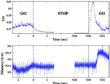
A typical result of such an experiment is given in Fig. 5. Let us first focus on the upper curve, which shows the evo-lution of the(dimensionless) tangential stress. Just after the stop, there is a small decrease in tangential stress and a very slow creep during the waiting time. When restarting the shearing, the interface resists elastically up to a maximum
value of the tangential stress. It means that during the stop under normal and tangential stress there has been an evolu-tion of the effective(static) friction coefficient. The system exhibits aging. If we pursue the displacement of the grains, sliding occurs and the tangential stress recovers its steady-state value, at the same level as before the stop. There is
rejuvenation of the granular layer under shearing.
Let us define⌬ as the difference between the value of
T / N at the peak and its value in the steady state. This
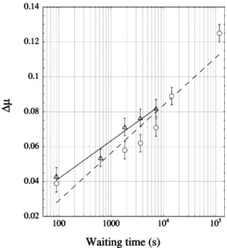
quan-tity is plotted as a function of the waiting time in Fig. 6; to estimate the error made in the measurements, ten identical stop-and-go experiments(same sample, same waiting time of 30 mn) have been done. The standard deviation of the mea-surements for the ⌬ peak and the relaxation time (see below) give the error bars in Figs. 6 and 7. The quantity⌬ increases roughly as the logarithm of the waiting time, and in all experiments the slope ranges in the interval关0.01,0.02兴 per unit logarithm. We do not observe any significant evolu-tion of the slope with the imposed driving velocity. This logarithmic increment of the effective static friction coeffi-cient has been observed by de Ryck et al.[5], with a slope of 0.01, for normal stresses of the same order of magnitude as in our experiment. It is also observed for a quartz gouge between granite blocks at high normal stress共25 MPa兲 with a slope 0.005[15,16]. In Fig. 6, we show two sets of data. Open circles correspond to experiments done just after sample preparation (pouring the grains and 30° rotation at FIG. 4. Left ordinate,䉭: characteristic length Lflucof the
fluc-tuations of normalized tangential stress(in cm), in the steady state, as a function of the driving velocity(inm/s). Right ordinate, 䊊: amplitude⌬共T/N兲 of those fluctuations as a function of the driving velocity. The inset shows the power spectrum of the tangential stress in the steady state(arbitrary units), as a function of the in-verse wavelength 1 /⌳ (in cm−1), and clearly exhibits a rather broad
peak, from which we calculate Lfluc⬃⌳⬇5 mm. For all data, the
normal stress is the same, N⬇9.73 kPa; the power spectrum is obtained for a driving velocity of 880m/s.
FIG. 5. Evolution of the normalized shear variation (upper curve) and dilatancy variation (lower curve, inm) with time, in a stop-and-go experiment. The resolution is 400 point/ s or 9 point/m. The sample is prepared under a normal stress of 9.73 kPa and a driving velocity of 44m/s. The dotted lines indi-cate the stop time共t⬅0 s兲 and the restart time 共t=7230 s兲. Here 3 s are shown just after the stop, and 2 s just before the restart, during the creep. In the upper curve, we show an exponential fit of the evolution of the tangential stress from its maximum value toward the steady state. The small “spikes” in the tangential stress data may be due to the motor. Their typical frequency is roughly 2 times the number of steps per seconds, and they disappear when the motor is stopped. The high-frequency oscillations, in the dilatancy data, are instrumental noise. They are related to the electronics, not to the motor, since they persist during the stop.
constant driving velocity). The logarithmic fit is not good at small waiting time. A curve of the same shape has already been observed by Losert et al.[14] (see their Fig. 5), for a stop-and-go experiment in a linear geometry, at comparable
driving velocity(28.7m or 0.25 d / s in units of their grain diameter) and waiting times, but a very small normal stress of 20 Pa.
This phenomenology is also observed in solid friction ex-periments [25,26]. In this context, the contact of the two rough solids occurs between microasperities, and aging is interpreted as a yielding of those microasperities under stress. This leads to an increase of the actual contact area between the two solids during the waiting time, hence an increase in the friction coefficient. Resuming the shear, slid-ing begins and the microcontacts are progressively destroyed and replaced by new contacts between fresh asperities. Slid-ing implies rejuvenation of the frictional interface. The phe-nomenological rate and state model of Dieterich, Rice, and Ruina [27,28] (DRR) has been introduced to describe the dependence of the friction coefficienton sliding velocity x˙ and on an internal variabledescribing the age of contacts. In this model, =0+ a ln x˙ V0 + b lnV0 Dc , 共2兲 d dt = 1 − x˙ Dc , 共3兲
where0 is the steady-state friction coefficient at constant sliding velocity V0, Dcis a characteristic length, and a and b
two material-dependent constants. Those equations must be completed by one describing the dynamics. Neglecting the inertia, this last equation may be written
K共V − x˙兲 = Wd
dt, 共4兲
where K is the spring stiffness and W is the weight supported by the grains.
FIG. 6. Plot of the friction coefficient peak ⌬ at restarting (linear scale), as a function of the waiting time (logarithmic scale). The two different symbols correspond to the same stop-and-go ex-periment, done on the same sample, just after sample preparation 共䊊兲 and after the first experiment 共䉭兲. The slope of the fit, which corresponds to the coefficient b of Eq.(2), is 0.010 in the first case and 0.012 in the second case. The velocity for sample preparation and restart was 22m/s, and normal stress was 10.78 kPa.
FIG. 7. (a) Plot of the characteristic time as a function of the waiting time, for stop-and-go experiments made at several different driving velocities V(䉮, 5.5m/s; 䊊, 11 m/s; 〫, 22 m/s; 쎲, 44 m/s; 䉭, 88 m/s). (b) Plot of the product ⫻V, as a function of the waiting time, for the same experiments(same symbols). It is clear that the data collapse around a mean value of 10m.
The state variable is basically the age of the contact. Without sliding—that, is x˙ = 0—= t and the model includes the logarithmic increase of the static coefficient of friction with contact time. Formally, there is a divergence in Eq.(2) at x˙ = 0 but any measurement of the friction coefficient im-plies that the surface undergoes slip at some scale[2]. Under constant driving velocity V, the steady-state solution of Eqs.
(2)–(4) is
x˙ = V, *= Dc/V, d=0+共a − b兲ln共V/V0兲. 共5兲
When sliding sets in, the structural age decreases from its initial value, after a waiting time twait, toward the smaller
value*reached in steady motion: the DRR model includes rejuvenation of the interface as well.
The sliding velocity is equal to the driving velocity V in the steady state. It is also the case just at the peak value[26]. Indeed, K共V−x˙兲=Wd/ dt = 0 just at the peak. Hence a rough estimate of the relaxation of is obtained if we assume x˙ = const= V. A small perturbation=*+␦evolves follow-ing d␦ dt = − V Dc ␦, 共6兲
which corresponds to an exponential relaxation with the characteristic time ⬅Dc/ V. Since ␦ is a small perturba-tion,is linear in␦and its relaxation toward steady state occurs with the same time scale . The length Dc is thus identified as the characteristic length necessary for contact rejuvenation to occur. In what follows, we will use those results obtained in a linear geometry, because as we said before the radius of the annular cell is much greater than its width and curvature effects may be neglected[5].
Let us focus now on the relaxation toward the steady state for the tangential stress in our granular system. As shown in Fig. 5, it is quite well described by an exponential fit. In the case of the figure, the characteristic time is 0.27 s. We made a systematic study of similar stop-and-go experiments, vary-ing only the drivvary-ing velocities. The results are displayed in Fig. 7. From Fig. 7(a), we see that this relaxation time is independent of the waiting time, but depends on the shearing velocity V. When we plot the product V, all the data col-lapse on a single curve as shown in Fig. 7(b). This means that the relaxation is described by a characteristic length, the value of which is about 10m. Another way to see this is to plot, averaged on all waiting times at a given angular ve-locity⍀, as a function of 1/⍀. This is done in Fig. 8.
The order of magnitude for Dcis microscopic, but much
larger than in the context of solid friction, where Dc ⬇0.5m, an order of magnitude roughly comparable with that of a microcontact between asperities[25]. A length scale much smaller than the bead radius and much greater than the typical size of asperities, which appears naturally in a granu-lar piling, is the size of the contacts between the grains. This latter may be roughly estimated if we consider that the nor-mal stress is borne by “columns” of grains. Let S be the area of the cell and d the mean grain diameter. There are roughly
S / d2 columns of grains that bear the normal force NS, for a normal stress N. The force on each column is thus Nd2.
Us-ing Hertz theory of the contact between spheres([29], Sec. 9), we get for the contact diameter a a value ranging between 8 and 12m, for normal stresses ranging between 3.3 and 11.3 kPa. This order of magnitude compares very well with that of Dc. We think that this comparison is relevant, because a column of grains behaves like a chain of frictional contacts, which before sliding behaves like a chain of springs resisting tangential stress. Sliding will occur at the weaker contact, relaxing the stress in the rest of the chain: the typical length necessary to relax the stress in the chain is thus the size of this weaker contact. This picture is of course oversimplified, because we consider only one column and sliding occurs on all the annulus surface. Nevertheless, we think that it is rea-sonable to consider that initially the sliding is concentrated on a single contact, rather than being shared among all con-tacts. We tried to exhibit a variation of Dcwith the normal
stress. It is not completely convincing, because of the rather large scatter in the data[see Fig. 7(b)] : we measure 9±3m for 3.3 kPa and 14± 3m for 11.3 kPa. The only thing that can be said with confidence is that it does not contradict our interpretation of Dc.
Let us finally discuss the evolution of the dilatancy, shown in the lower curve of Fig. 5. If we consider what happens when we restart the driving, it is perfectly clear, and observed in every such experiment, that the dilatancy does not evolve during the elastic reloading of the granular layer. It means that configurational rearrangements of the grains do not occur in the granular layer at a significant level until the beginning of sliding. The dilatancy evolution at the resuming of sliding is very small, even smaller than typical fluctua-tions in the steady state. Moreover, it does not depend on the waiting time, as shown in Fig. 9. This is another piece of FIG. 8. Plot of the characteristic time taken by the tangential stress to evolve toward its stationary value, averaged over all wait-ing times, as a function of the inverse angular drivwait-ing velocity 1 /⍀. The error bars are the standard deviation around the mean value.
evidence that, during the stop, basically no structural rear-rangement occurs in the granular layer.
This is consistent with our previous picture of “columns” of grains, in which contacts are established between grains in such a way that they support the weight of the cover. They age during the waiting time, and when we resume the shear they respond elastically, up to a maximum stress. Then slid-ing occurs, and the dilatancy evolves. This picture is sup-ported by the results of Utter and Behringer et al.[12]. In a 2D Couette experiment at constant volume, with photoelastic grains, they visualize the stress distribution at the grain scale during a stop-and-go experiment. This distribution is not ho-mogeneous, but rather concentrated along stress chains. Those stress chains, established in the steady state, are al-most not perturbed during the wait, neither by restarting the shear in the same direction as before the stop. The lack of large grain rearrangements in their observations is consistent with the lack of dilatancy variations during the stop which is seen in our experiments. Aging, as evidenced by the peak in tangential stress at restarting shown in Fig. 5, is thus not explained by structural rearrangements of the piling, but rather by the behavior of contacts between grains.
When the contacts are between plastic materials, such as contacts between microasperities of PMMA blocks[25], or between quartz grains at very high normal stress[3,7], aging may be interpreted as due to yielding at contacts, which in-creases the actual contact area, hence the strength of the contact. This is difficult to invoke for brittle material such as glass. Aging at the contacts may be due to some contami-nants or to condensation of water vapor.
C. Velocity jumps
In the Dieterich-Rice-Ruina model(2), the friction coef-ficient depends on the sliding velocity. A velocity jump from
V−to V+should lead to a variation of the steady state friction
coefficient:
⌬stat=共a − b兲ln
V+ V−
. 共7兲
A sudden change of velocity is not necessary to observe this effect, which expresses the fact that the steady-state friction coefficient depends on the sliding velocity. We may use the data already used for Fig. 4, since they were obtained for several sliding velocities, but only one initial density. In Fig. 11(a), below, we plot the effective friction coefficient, aver-aged on a large sliding distance(typically 3 cm), as a func-tion of the sliding velocity. The data are consistent with the DDR model, but the error bars, which are given by the am-plitude of fluctuations displayed in Fig. 4, are quite large. In this respect, velocity jump experiments give better results.
If the velocity jump is instantaneous, there is another ef-fect: The value of just after the jump is unchanged, = Dc/ V−, and there is an instantaneous increment in the
fric-tion coefficient
⌬inst= a ln
V+
V−
. 共8兲
The relaxation from the peak⌬insttoward the steady state at
velocity V+,⌬stat, takes places on a characteristic distance
equal to Dc[2].
We thus perform (quasi-)instantaneous velocity jumps, from V−to V+⬎V−. The sample is prepared by initial shear-ing at uniform drivshear-ing velocity V− during a 30° rotation.
Then, we perform series of jumps with the same V−, and
several values of V+, in increasing and then decreasing order
(typically from 0.2 up to 1.8 mm/s). We make sure that the
large velocity displacement is sufficient to reach a steady state.
A typical experimental result is given in Fig. 10, showing the(dimensionless) tangential stress in the upper curve, the dilatancy in the lower. We do observe the variation⌬statof
the stationary values for the effective friction coefficient. The granular layer is velocity strengthening (i.e., the tangential stress increases with the velocity). Our velocity jumps are performed after large cumulated shear displacements, 6 cm or 40 bead diameter for each data point, and we always do observe velocity strengthening of the granular layer. This was not the case in the experiments of Mair and Marone[7], who observed a transition from a first velocity strengthening regime toward a velocity weakening one, for a displacement of 100 grain diameters. But in the case of their experiments, they begin the velocity jumps before reaching the steady state. Their velocity strengthening regime is a transient, dif-ferent in nature from the one that we observe.
In Fig. 11(b), we plot the evolution of the variation of friction coefficient with the higher velocity V+, for several lower velocities V−. The data follow a logarithmic evolution,
and when plotted as a function of the ratio V+/ V− they
col-lapse onto a single curve, in agreement with the DRR model FIG. 9. Plot of the dilatancy variation after restarting as a
func-tion of waiting time, in logarithmic scale. The data correspond to the same experiments as in Fig. 6, and the symbols have the same significance. The variation of dilatancy is always very small (com-pared either to a mean level of 350m or to fluctuations about ±5m; see Fig. 2) and independent of the waiting time.
(7) [see Fig. 11(c)]. The data are consistent with those of Fig.
11(a), which are obtained in a completely different way. The slope, equal to a − b in the model, is 0.036 and ranges in the interval [0.03 0.05] in all experiments. With our previous measurement of b, this means that a ranges in the interval
[0.04 0.07].
We may compare our results to those of the geophysicists
[2,3,7], and those of Géminard et al. [8]. Those experiments
are quite similar, except for the normal stress which is very low in[8], typically 20 Pa, and very high in [2,3,7], typically 25 MPa, to be compared to the order of magnitude of the normal stress in our experiments, 30 kPa. Those stresses may be compared directly because the Young’s moduli Y of the grains, either glass bead as in the present work ([8], Y
= 60 GPa) or granite ([2,3,7], Y苸关50,70兴 GPa), are very similar.
No evolution of the friction coefficient is observed in[8], with a velocity varying over four orders of magnitude, from 0.1 up to 1000m / s, or 10−3 up to 10 bead diameters per
second. Under high stresses, both instantaneous increment
⌬inst and steady-state increment ⌬stat are observed in
[2,3,7]. We do not see the instantaneous increment⌬instin
our experiment, in contrast with the DRR model, Eq.(8). The instantaneous increment⌬inst is linked to the state variablethat describes aging in Eqs.(2) and (3). Since we do observe aging in our system, it is quite puzzling not to see any instantaneous increment. We will thus discuss at length the possible explanations for our result.
The space resolution of the data is at least 0.11m be-tween two points, at velocity V+. This is much less than the
value of Dc⬇10m, so that a lack of resolution is not a relevant explanation.
The variations of friction coefficient are rather small com-pared to the fluctuations in the steady state, and we must make large changes in velocity(by a factor of 20, typically). It is thus not obvious that the velocity change is actually instantaneous. The rotation is ensured by a stepping motor, and the maximum angular acceleration is 0 to 0 – 40° / s in 250 ms, hence V˙max= 0.3 m / s2. In all cases, the low velocity
is negligible. For a high velocity ranging from 0.2 up to 1.8 mm/ s, the duration of the accelerated motion ranges be-tween 0.36 and 5.7 ms, corresponding to a distance bebe-tween 0.02 and 5.1m. Even in the worst case, this distance is less than Dc(for the case of Fig. 10, the motion is accelerated for
the first 1.25m, much less than Dc). Hence it does not seem that an insufficient acceleration should be the explana-tion.
Assuming that the instantaneous change of driving veloc-ity creates a sudden jump in friction, this implies further deformation of the cantilever spring, hence the motion of the cover plate. The typical time scale for cover motion is
冑
m /共2k兲, where the factor of 2 comes from the moment ofFIG. 10. Example of velocity jump; the upper curve shows the tangential stress, the lower curve the dilatancy, inm, as functions of time, in s. The low velocity is V−= 11m/s 共t⬍0兲, the high velocity is V+= 880m/s 共t⬎0兲. The normal stress is 9.73 kPa.
The time origin is taken at the jump V−→V+. The amplitude of
dilatancy variation should be compared to the dilatancy fluctuations in steady state, typically ±5m (see Table I), and to the dilatancy variation in a stop-and-go experiment(see Fig. 9).
FIG. 11. (a) Value of the effective friction coefficient 具典 (averaged over a large distance, typically 3 cm), in the steady state, as a function of the velocity V in a logarithmic scale. Data are the same as those used in Fig. 4. Note that error bars(typically ±0.05) are much lager than in the case of(b) (typically ±0.02), due to the measuring process. (b) Value of the increment of effective friction coefficient⌬stat
for a velocity jump V−→V+, in the steady state, as a funtion of V+. The abcissa is given in a logarithmic scale, for several values of V−:
V−= 5.5m/s (solid triangles), V−= 11m/s (soild circles), and V−= 22m/s (solid squares). (c) Same data, with the same symbols, but
plotted as functions of the ratio V+/ V−, in logarithmic scale. All data collapse on a single curve. The normal stress is 9.73 kPa. The error bars are estimated from the fluctuations of T / N. For(a), those fluctuations are displayed in Fig. 4. For (b) and (c) they are much less since they are calculated on a much shorter distance.
inertia of a plain disk of mass m. In the case of Fig. 10, m = 9.6 kg and this time scale is only 2.5 times less than Dc/ V;
it is not obvious to consider the cover motion as instanta-neous, so that we cannot exclude completely inertial effects. The physical reason for the instantaneous jump⌬inst, in
the context of solid friction, is that the system has to slide on a distance Dcfor the complete renewal of asperities[27]. In
experiments on granular gouge[2,3,7], the thinest granular particles created by wear of the rocks surface and comminu-tion of the initial grain layer should play the role of the asperities. Such phenomena are not relevant for our experi-ments, which are done at much smaller normal stresses. An-other point is that, in order to see aging in our system, we have to wait typically hundreds of seconds: no effect is seen for a waiting time of 1 or 10 s. The steady state value*, for a sliding at the lowest velocity of 5m / s, is 2 s, which is probably not enough to see any effect.
A careful measurement of the coefficient a of Eq.(2) has been made by de Ryck et al.[5], and they found good agree-ment between the model and their data. They used an annular shearing box, normal loads comparable to ours, and siliga gel grains of typical size 0.1 mm. But they measured a during the creep in a stop-and-go experiment, not by imposing ve-locity jumps on the grains. In the creep phase, the response of the granular layer is mainly due to the behavior of the frictional contacts, without significant rearrangements of grains, which is definitely not the case for a velocity jump.
As shown by Fig. 10, an increment of dilatancy follows a driving velocity jump. Such a dilatancy increment has been observed by Mair and Marone[7], but not by Géminard et al.
[8]. It is very difficult to compare those results, because of
the very different orders of magnitude for the normal stresses. In the experiments of Mair and Marone [7], the grains are progressively broken and the granularity is not constant during the shearing, which is not the case in our experiment. They nevertheless measure a dilatancy incre-ment of typically 2% of the mean grain diameter, for
V+/ V−= 10 and a layer of 40 grains. This is roughly the same
in our experiments(see Fig. 12; the increment is 10m for
V+/ V−= 20 and a layer of 15 grains). The lack of dilatancy
increment when varying the driving velocity, evidenced in the experiments of Géminard et al.[8], is probably due to the very low normal stress in their experiments. In fact, they always observe a smaller dilatancy than we do. When they shear freshly poured grains at constant driving velocity, the dilatancy increment is 5m or d / 20, for a layer of depth 30d, in units of the beads diameter d. In the same kind of experiment, we obtain a dilatancy of d / 3 for a layer of 15d. The dilatancy increment depends on the amplitude of the driving velocity jump. The evolution of the dilatancy is shown in Fig. 12, as a function of V+/ V−. It evolves
logarith-mically, with slope 13m per unit of the quantity ln共V+/ V−兲.
The dilatancy variation (typically 50m) is significantly greater than the dilatancy fluctuations in steady state
共±5m兲. However, this variation is quite small when com-pared to the dilatancy of freshly poured grains (typically 500m). For V+/ V−⬇100, the dilatancy increment is about
50m. Dividing by the number 共⬇10兲 of granular layers below the teeth extremities, we get 5m, which is compa-rable to the roughness of the beads. Thus the mecanism of
the dilatancy variation during a velocity jump may be related to the behavior of individual frictional contacts, whereas the shearing of freshly poured grains necessarily involves struc-tural rearangements of the grains.
IV. CONCLUSION
We have studied the low-velocity shearing of a confined granular layer. The dimensionless shear rate varies between 10−6and 10−4[Eq. (1)].
A first result is the evidence that the response of the granular layer under shearing is described by characteristic
length scales, not time scales. Those length scales describe
the evolution of the layer toward a steady state and the stress fluctuations when this steady state is reached. Importantly, the steady state for tangential stress is reached on the same length scale as that for dilatancy. It shows that there is an intricate coupling between the tangential stress variations and those of dilatancy, or free volume.
When the driving is stopped and the grains are kept under normal and tangential stress, the system ages, showing a logarithmic increase of static friction coefficient with waiting time. There is no evolution of the dilatancy during either the stop or elastic reloading of the granular layer at the begining of restart. Aging is thus not due to structural rearrangements of the granular layer, which would imply changes in density. The contacts between the grains, established at the stop and supporting the stress during the waiting time, are responsible for aging.
Resuming the shearing, there is rejuvenation of the sys-tem. Several experiments, done at different driving veloci-ties, provide evidence that this rejuvenation occurs with a FIG. 12. Plot of the increment of dilatancy, inm, for a velocity jump V−→V+, as a function of the ratio V+/ V−in logarithmic scale.
characteristic length that may be identified with the
param-eter Dc of the Dieterich-Rice-Ruina model. We find Dc
⬇10m, which is the order of magnitude of a Hertz contact between adjacent grains. The cover plate, during the waiting time, is held by several chains of contacting grains. Each contact resists to shear up to a maximum value, and the chains are broken when the weakest contact breaks. A length scale of the order of the lateral size of a Hertz contact is thus sufficient for this process to take place everywhere in the cell, such that sliding occurs and rejuvenates the granular layer.
When driving velocity jumps are imposed on the grains, the system exhibits velocity strengthening behavior. The variation of friction coefficient, in the steady state, is a loga-rithmic function of the upper velocity V+. Data obtained for
several lower-velocity V−collapse onto a single curve when
plotted as a function of ln共V+/ V−兲. No instantaneous increase
is observed for the friction coefficient. This cannot be related to a poor resolution, neither to insufficient acceleration.
When the higher velocity is kept constant on a sufficient distance, a steady state is reached for the dilatancy, and the dilatancy increase is a logarithmic function of V+/ V−. The
order of magnitude of this effect indicates that the response of the layer probably does not involve structural rearrange-ments of the grains.
With our experimental protocol, the stop-and-go and ve-locity jump experiments are done when the shear band is fully established. In this regime, our measurements are well described by the Dieterich-Rice-Ruina model[21,22], which does not include the dilatancy, which thus appears as a slaved variable. On the contrary, the dynamics of shear band building, just after filling the cell, exhibits a strong coupling between tangential stress and dilatancy.
ACKNOWLEDGMENTS
I thank A. de Ryck and A. Lemaître for useful discussions. I am indebted to T. Baumberger and C. Caroli for a critical reading of the manuscript and many useful remarks.
[1] R. M. Nedderman, Statics and Kinematics of Granular
Mate-rials (Cambridge University Press, Cambridge, England,
1992).
[2] C. Marone, Annu. Rev. Earth Planet Sci. 26, 643 (1998). [3] N. M. Beeler, T. E. Tullis, M. L. Blanpied, and J. D. Weeks, J.
Geophys. Res. 101, 8697(1996).
[4] M. Lubert and A. de Ryck, Phys. Rev. E 63, 021502 (2001). [5] A. de Ryck, R. Condotta, and M. Lubert, Eur. Phys. J. E 11,
159(2003).
[6] S. Shibuya, T. Mitachi, and S. Tamate, Geotechnique 47, 769 (1997).
[7] K. Mair and C. Marone, J. Geophys. Res. 104, 28899 (1999). [8] J.-C. Géminard, W. Losert, and J. P. Gollub, Phys. Rev. E 59,
5881(1999).
[9] J.-C. Tsai, G. A. Voth, and J. P. Gollub, Phys. Rev. Lett. 91, 064301(2003).
[10] G. Chambon, J. Schmittbuhl, A. Corfdir, J. P. Vilotte, and S. Roux, Phys. Rev. E 68, 011304(2003).
[11] D. Fenistein and M. Van Hecke, Nature (London) 425, 256 (2003).
[12] B. Utter and R. P. Behringer, Eur. Phys. J. E 14, 373 (2004). [13] R. R. Hartley and R. P. Behringer, Nature (London) 421, 928
(2003).
[14] W. Losert, J.-C. Géminard, S. Nasuno, and J. P. Gollub, Phys. Rev. E 61, 4060(2000).
[15] S. L. Karner and C. Marone, Geophys. Res. Lett. 25, 4561 (1998).
[16] N. M. Beeler and T. E. Tullis, J. Geophys. Res. 102, 22595 (1997).
[17] S. Torquato, T. M. Truskett, and P. G. Debenedetti, Phys. Rev. Lett. 84, 2064(2000).
[18] J. Duran, Sables, Poudres et Grains (Eyrolles, Paris, 1997). [19] GDR MiDi Collaboration, Eur. Phys. J. E 14, 341 (2004). [20] S. Douady and A. Daerr, in Physics of Dry Granular Media,
edited by H. J. Herrmann, J.-P. Hovi, and S. Luding(Kluwer, Dordrecht, 1998).
[21] A. Lemaître, Phys. Rev. Lett. 89, 064303 (2002). [22] A. Lemaître, Phys. Rev. Lett. 89, 195503 (2002).
[23] J. Desrues, R. Chambon, M. Mokni, and F. Mazerolle, Geo-technique 46, 529(1996).
[24] M. Oda and H. Kazama, Geotechnique 48, 465 (1998). [25] T. Baumberger, P. Berthoud, and C. Caroli, Phys. Rev. B 60,
3928(1999).
[26] L. Bureau, T. Baumberger, and C. Caroli, Eur. Phys. J. E 8, 331(2002).
[27] J. Dieterich, J. Geophys. Res. 84, 2161 (1979).
[28] J. R. Rice and A. L. Ruina, J. Appl. Mech. 50, 343 (1983). [29] L. D. Landau and E. M. Lifshitz, Theory of Elasticity