HAL Id: hal-00945036
https://hal.archives-ouvertes.fr/hal-00945036
Submitted on 11 Feb 2014
HAL is a multi-disciplinary open access
archive for the deposit and dissemination of sci-entific research documents, whether they are pub-lished or not. The documents may come from
L’archive ouverte pluridisciplinaire HAL, est destinée au dépôt et à la diffusion de documents scientifiques de niveau recherche, publiés ou non, émanant des établissements d’enseignement et de
To cite this version:
Nicolas Canry, Julien Fouquau, Sebastien Lechevalier. Sectoral Price Dynamics in Japan: A Threshold Approach. Economics Bulletin, Economics Bulletin, 2011, 31 (2), pp.1322-1335. �hal-00945036�
Volume 31, Issue 2
Sectoral Price Dynamics in Japan: A Threshold Approach
Nicolas Canry Paris 1 University Julien Fouquau
Rouen Business School and CGEMP-LEDa
Sébastien Lechevalier
EHESS
Abstract
This paper focuses on the real – as opposed to the monetary – side of the economy to explain price dynamics in Japan between 1981 and 2001. We use a panel industry dataset to examine the impact of institutional and structural factors on the heterogeneous price dynamics in 10 manufacturing sectors. Although the evolution of unit labor costs may seem to be the driving force of these price dynamics, our analysis underlines the importance of the increasingly competitive environment, as captured by rising import penetration. Along with the decline of bargaining power of the workforce, this is a key factor underlying the deflationary pressures that characterized Japanese manufacturing industries in the 1990s.
1
IntroductionDeflation in Japan has attracted the attention of many researchers. Beyond the debate on economic policies, contributions have investigated various di-mensions such as monetary aspects, the impact of the banking crisis, and the microfoundations of price dynamics (for a survey see Smith, 2006). How-ever, to our knowledge, very few studies have examined the price dynamics at the sectoral level and its determinants, even though it has been recog-nized that deflationary pressures have been stronger and started earlier in the manufacturing than in the non-manufacturing sector (Baig, 2003).
The aim of this paper is to provide an analysis of the price dynamics at the sectoral level by focusing on manufacturing industries and analyzing their institutional determinants. In this approach, which focuses on the real – as opposed to the monetary – side of the economy to explain deflation, we disentangle what is related to the goods market and labor market dynamics, respectively, instead of using, as Saxonhouse (2005), for example, does, the concepts of demand-led versus supply-led deflation. In doing so, we aim at adopting a critical view on previous simple statistical decompositions of price dynamics that seemed to indicate that the evolution of unit labor costs was the driving force of the price dynamics in the Japanese manufacturing industries (see for example Canry et al., 2007). Investigating price dynamics at the sectoral level involves a triple challenge which may explain why there are few studies that have done so.
Specifically, doing so requires simultaneously taking into account the het-erogeneity of this dynamics among sectors, the temporal instability of the relationship, and more generally its potential non-linearity. There are vari-ous solutions to these issues in a panel framework. The solution we propose here is to adopt a non-dynamic panel transition regression model with fixed individual effects, namely the framework introduced by Hansen (1999). To our knowledge, this paper is the first attempt to apply this framework to the analysis of price dynamics at the sectoral level. Besides the methodological dimension, a second contribution of our paper appears in the results: we shed light on the existence of threshold effects for some institutional deter-minants of price dynamics in Japan, especially the international openness of the economy.
The paper is organized as follows. The following section presents the institutional determinants of price dynamics that we examine in this paper and introduces the threshold approach as an extension of a simple linear approach. The results are then presented in Section 3, while Section 4 con-cludes.
2
Institutional determinants of price dynamics at the sectoral level: from a linear to a threshold approachOver the last decades, the literature on the impact of institutional factors on both goods and labor markets has grown rapidly. Based on this litera-ture (e.g., Nickell, 1999; Oliveira-Martins et al., 1996; Boulhol et al., 2006, Abraham et al., 2009), we select a number of variables that characterize the structure of the labor and goods markets and – through their effect on markups and the bargaining power of the workforce – potentially affect price dynamics at the sectoral level1. To characterize the structure of the goods
market, we use two variables. First, we use an index of regulation, regi,t, by
sector taken from the Japan Industry Productivity database (RIETI). This index, which has been widely used in studies investigating issues related to goods market regulation, takes a value from 0 to 1 (from least regulated to most regulated) and we expect prices to be positively correlated with it as regulation negatively affects market entry and therefore creates oligopolistic rents. The second variable related to the goods market is the degree of im-port penetration, impi,t. Taken from the OECD’s STAN database, this aims
at capturing the degree of market openness in a particular industry2. The
impact of this variable on prices is straightforward: the more open a market is, the lower should the markup rates and therefore prices be.
As for the the labor market structure, the bargaining power of unions is captured through the number of labor disputes, dispi,t, variable provided
by the Ministry of Health, Labour, and Welfare (MHLW). Another variable, taken from the same source, is the job vacancy rate, vac rati,t, (the ratio of
the number of vacant positions to the number of persons looking for a job). It is available at the sectoral level and is expected to affect positively the bargaining power of the workforce and therefore prices. Its usefulness as an advanced indicator of the bargaining power of the workforce has been shown by Minami (1994). A third variable, provided by the MHLW, is the share of part-time workers in the sectoral workforce, ptimei,t. An increase in this
share should negatively affect the bargaining power of unions.
Finally, we introduce two control variables: productivity, prodtyi,t, and
the money supply, M2t. We have an annual balanced panel of 10 sectors
for the period 1981-2001. This allows us to compare the 1990s, a period
1We initially included other variables, such as the number of firms, the average size of
firms, and the unionization rate, which, however, were not significant and are therefore not included here.
2Import penetration is widely considered as a good proxy of the degree of market
when the majority of sectors experienced falling prices (see Table 1), with the 1980s. Table 2 provides summary statistics of the variables.
Using these variables, we employ the following linear specification, ex-pressed in log-form:
Pi,t= µi + α1prodtyi,t+ α2regi,t+ α3impi,t+ α4vac rati,t (1)
+ α5dispi,t+ α6ptimei,t+ α7M2t+ ǫi,t
where Pi,t is the price in sector i and period t, µi the individual effect and
ǫit is a stochastic error term. Let us highlight a potential problem in this
model. Obviously, there are unobservable factors affecting prices that are not taken into account in this model.This may lead to an endogeneity problem if omitted variables (e.g., sectors unobservable characteristics) create correla-tion between one or more of the regressors and the error term. The inclusion of a variable to capture sector fixed effects, µi should resolve this issue.
Moreover, the model described in (1) has two major drawbacks: 1) it assumes that the impact of structural variables on prices is constant during the 21-year period; and 2) it assumes that all sectors are characterized by the same dynamics. To relax these highly improbable assumptions, we follow Hansen’s (1999) procedure. More precisely, we use a non-dynamic Panel Threshold Regression model (PTR), which can be considered as an extension of the linear specification:
priceit = µi+ β1XitI (qit ≤γ) + β2Xit I (qit > γ) + ǫit, (2)
where qitis the threshold variable,3 γa threshold parameter, Xit the vector of
explanatory variables described in the previous section and I(.) an indicator function which takes a value of 1 when the threshold condition in the brackets is satisfied and 0 otherwise. Then, the observations are divided into two regimes depending on whether the threshold variable qit is smaller or larger
than the threshold parameter γ. The regimes are distinguished by different regression slopes, β1 and β2. Moreover, there is no reason to limit our analysis
to only two regimes. The estimation approach proposed by Hansen allows a more general specification with r thresholds (i.e., r + 1 regimes).
A first advantage of this model is that, conditional on the number of regimes, it allows parameters to vary across individuals (heterogeneity issue) and also over time (stability issue). For our specific purpose, the PTR model
3No constraints are imposed on the choice of the threshold variable except that it
cannot be a contemporaneous endogenous variable and it cannot be time constant. The choice of this threshold variable is discussed further below.
has a second great advantage: it allows us to identify potential threshold effects in price dynamics. More precisely, we test whether an exogenous variable has contributed to a significant change in the price dynamics in the 1990s. This issue exactly corresponds to what the PTR model has been designed for.
The estimation procedure is as follows. First, estimation of the model pa-rameters requires eliminating the individual effects µiby removing
individual-specific means and then applying the least squares sequential procedure (see Hansen, 1999, or Fouquau, 2008, for more details). For a given value of the threshold parameter γ, the slope coefficients β1 and β2 in (2) can be
esti-mated by OLS. The resolution of the sum of squared residuals minimization problem can be reduced to a search over the values of γ equal to the distinct values of qit in the sample.4
The next step is to determine whether the threshold effect is statistically significant relative to a linear specification. The null hypothesis in this case describes the simple linear specification and can be expressed as H0 : β1 = β2.
In a standard framework, this hypothesis could be tested by a standard likelihood ratio test,
F1 =
S0 −S1(ˆc)
ˆ
σ2 , (3)
where S0 is the sum of the squared residuals of the linear model, S1 the sum
of the squared residuals of the one-threshold model, and ˆσ2 = S1(ˆc)
n(T −1).
Unfor-tunately, the distribution of this test is non-standard since the PTR model contains unidentified nuisance parameters γ under H0. A possible solution
is to simulate by bootstrap the asymptotic distribution of the statistic F1.
If the threshold effect is proven, the same procedure can be applied in order to determine the number of thresholds required to capture the whole non-linearity. The new null hypothesis consists of testing a specification with r regimes versus a specification with r + 1 regimes. The procedure starts by testing one threshold versus two, then two versus three, and so on. The procedure stops when the null hypothesis is not rejected.
3
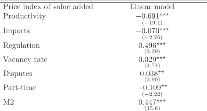
ResultsWe first report in Table 3 the estimation of the linear regression (equation 1), which serves as a benchmark. All the variables are significant and have the
4It is undesirable to select a threshold c which leads to too few observations in a
particular regime. Therefore, we impose at least T /2 observations in a given regime. This ensures that the influence of a given sector in the search for c is not neglected.
expected sign. However, for the reasons previously mentioned, it is necessary to extend this linear estimation in adopting the threshold approach.
A key issue in estimating the PTR model is identifying the appropriate threshold variables to capture the model’s non-linearity. Potentially, all the explanatory variables of the price dynamics we consider in this paper are can-didates to be the threshold variable, which may explain the regime changes. However, we do not consider here M2, which is a control variable and which does not have any individual dimension. Similarly, ex ante, we exclude the regulation index as a potential candidate for the threshold variable because of the following empirical features: 1) some sectors exhibit only zeros; 2) the variable is characterized by a high stability over time5. Therefore, it cannot
explain regime change, which is the main concern of this paper.
Then, there are theoretical and empirical criteria that justify our final choice of the threshold variables among all the remaining candidates. On the theoretical side, previous studies have especially emphasized the role of three variables to explain structural changes that characterized the Japanese economy in the last decades: productivity (Yoshikawa, 2002), vacancy rate (Minami, 1994) and import penetration (Boyer & Yamada, 2000). We will nonetheless consider all the remaining candidates and adopt statistical cri-teria to select the threshold variable.
More precisely, on the empirical side, we apply two complementary cri-teria to determine the optimal threshold variable: we select the threshold variable which minimizes the sum of squared residuals (see Hansen, 1999) and which leads to the strongest rejection of the linearity hypothesis (see Gonzalez et al., 2005). Based on these two criteria, the best models are, in order, the ones with productivity and import as the threshold variable (Table 4)6.
Finally, a third criterion should be taken into account: the choice of the threshold ultimately depends on how much it allows us to take into account not only the individual (sectoral) heterogeneity but also the regime changes. When productivity is the threshold variable, we can capture the heterogeneity across sector but not well the evolution over time and the regime changes7.
5These empirical features are not reproduced here because of space constraints but are
available from the authors upon requests.
6At the same time, it is worth noticing that in all cases, the linearity tests (F1) clearly
lead to the rejection of the null hypothesis of linearity of price dynamics with a bootstrap p-value smaller than 0.01. This result confirms the nonlinearity of sectoral price dynamics in Japan, which by and of itself justifies the adoption of the PTR model.
7One additional reason is the following: what has been observed in Japan since the
early 1990s is a productivity slowdown, which may hardly explain deflationary pressures (Yoshikawa, 2002).
By comparison, when import penetration is the threshold variable, we can capture much better the regime changes, while we also take into account the individual heterogeneity, as it can be seen in the Figure 18. This is the
final reason why import penetration is the optimal threshold variable for our purpose.
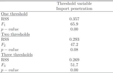
Once the threshold variable has been selected, the next step is to deter-mine the optimal number of regimes. In table 5, the likelihood ratio tests F2 and F3 are also significant at a level of 10% for the two variables. Thus, there are at least four regimes9.
The estimates of the parameters of the PTR model and the threshold values are reported in Table 6. These parameters show when the transition between two regimes occurred. For instance, if the logarithm of the import penetration is more than 1.27, the sector concerned switches to the second regime. According to these values, we can deduce the distribution of the sectors among the different regimes (Figure 1).
Before going into the details of the results, the following preliminary comment is in order. First, one observes that, in all sectors, the import penetration variable is higher in 2001 than in 1981, indicating an increase in the openness of Japanese manufacturing industries. Therefore, this variable allows us to capture the evolution of the whole structure over time. Second, our framework also allows us to capture the cross-sectional heterogeneity in that it clusters all the sectors with the same import penetration (Figure 1). All the seven variables we analyze are significant in at least one regime and the bulk of them have the expected sign when they are significant, but their significance varies depending on the regime (Table 5). In all four regimes, the impact of labour productivity and the money supply (M2) on prices is highly significant (at the 1 % level). As for import penetration, it becomes significant (with the expected negative sign) in the third and fourth regimes. This can be interpreted as follows: an increase in import penetration has no effect on prices when the degree of openness of a sector remains low (an im-port penetration ratio of less than 6.2 % according to the value of the second threshold). The number of disputes and the share of part-time workers both have the correct sign when they are significant, which confirms the results obtained with the linear specification, but also shows that these results are
8The results with productivity as the threshold variable are available from the authors
upon reques
9According to Hansen’s procedure, it would be necessary to estimate and test four
thresholds, five thresholds and so on, until the corresponding F-test is statistically in-significant. However, we limit our analysis to a model with at most four regimes. This choice can be justified by the fact that it does not affect (or only slightly affects) the estimates of the other threshold parameters.
conditional on the level of import penetration. We do not discuss this point further since it would require more research along the lines of Dobbeleare (2004), who examined the complementarity between labor market and goods market variables.
Finally, two coefficients, which are significant, have the wrong sign: the vacancy rate has a negative and significant impact in the first and the fourth regime, while the regulation index has a negative and significant impact in the fourth regime, contrary to our expectations and the results in the linear estimation. As for the regulation index, a possible explanation is that its impact is very strong and significant in the first regime (0.98), but then declines (while still being significant) in the second and third regimes (approximately 0.3). This result is consistent with what we expected: in the first regime, which basically corresponds to the initial situation with a low import penetration, the regulated structure of the goods market leads to high prices. This impact decreases as import penetration increases. In the fourth regime, the impact of regulation is still significant but becomes negative, possibly because this fourth regime includes two sectors for which the regulation index is always zero.10 As for the vacancy rate, this is the only
variable for which we have been unable to find a satisfying explanation for the result at this stage.
Overall, our analysis shows the importance of the increasingly competi-tive environment in the goods market. More precisely, we demonstrated that import penetration significantly affected price dynamics. Differences in reg-ulation across sectors are another factor that explains the heterogeneity in price dynamics. However, the level of regulation has not changed over time when considering the manufacturing sector as a whole see (see Table 2).
4
ConclusionThis article proposed an empirical framework to analyze sectoral price dy-namics in Japan. More precisely, we estimated the impact of institutional and structural factors in the labor and goods markets on price dynamics. Moreover, by using - for the first time for this specific issue, to our knowl-edge - a threshold approach in a panel framework, we were able to detect regime changes and to provide a richer economic interpretation than in a linear framework.
Overall, our results can be summarized as follows. Although simple
sta-10It is possible to plot the transition between regimes with respect to time and sector.
These plots, which make the interpretation of the results clearer, are not reproduced here because of space constraints but are available from the authors upon request.
tistical decompositions of price dynamics seem to indicate that the evolution of unit labor costs was apparently the driving force of the price dynamics in Japanese manufacturing industries (see Canry, Fouquau and Lechevalier, 2007), our analysis shows the importance of the increasingly competitive en-vironment in the goods market. More precisely, we demonstrated that import penetration significantly affected price dynamics by showing that the import penetration variable affects the price variable both directly and indirectly as a threshold variable at the origin of regime changes in these price dynam-ics. Differences in regulation across sectors are another factor that explains the heterogeneity in price dynamics. However, our simple statistical analysis presented in Table 2 showed that the level of regulation has not changed over time when considering the manufacturing sector as a whole. That is why it is possible to conclude that, along with the decline in the bargaining power of the workforce (as captured by the decreases in the vacancy rate, the number of disputes, and the share of regular employees), the increasing openness of the Japanese economy is a key factor underlying the deflationary pressures in manufacturing industries which characterized the Lost Decade. On the whole, our analysis shows that, in general, economists need to take into account the role of the labor market and the goods market when con-sidering price dynamics in Japan. Adopting a PTR model provides part of the solution.
5
References• Abraham, F., J. Konings and S. Vanormelingen (2009) “The Effect of Globalization on Union Bargaining and Price-Cost Margins of Firms,” Review of World Economics 145(1), 13-36.
• Baig, T. (2003) “Understanding the Costs of Deflation in the Japanese Context,” IMF Working Paper 03-215.
• Boulhol, H., S. Dobbelaere and S. Maioli (2006) “Imports as Product and Labor Market Discipline,” IZA Discussion Papers 2178.
• Boyer, R., and T. Yamada (2000) Japanese Capitalism in Crisis: A Regulationist Interpretation, London and New York: Routledge. • Canry, N., J. Fouquau and S. Lechevalier (2007) “Price Dynamics in
Japan (1981-2001): A Structural Analysis of Mechanisms in the Goods and Labor Markets,” IER Discussion Paper Series A 493, Hitotsubashi University.
• Dobbelaere, S. (2004) “Estimation of Price-Cost Margins and Union Bargaining Power for Belgian Manufacturing,” International Journal of Industrial Organization 22(10), 1381-1398.
• Fouquau, J. (2008) “Threshold Effects in Okun’s Law: A Panel Data Analysis,” Economics Bulletin 5(33), 1-14.
• Hansen, B. E. (1999) “Threshold Effects in Non-Dynamic Panels: Es-timation Testing and Inference,” Journal of Econometrics 93, 345-368. • Minami, R. (1994) The Economic Development of Japan: A
Quantita-tive Study, Basingstoke: Macmillan.
• Nickell, S. (1999) “Product Markets and Labour Markets,” Labour Eco-nomics 6(1), 1-20.
• Oliveira-Martins, J., D. Pilat and S. Scarpetta (1996) “Mark-Up Ra-tios in Manufacturing Industries: Estimates for 14 OECD Countries,” OECD Economics Department Working Papers 162.
• Saxonhouse, G. (2005) “Good Deflation/Bad Deflation and Japanese Economic Recovery,” International Economics and Economic Policy 2(2), 201-218.
• Smith, G. W. (2006) “The Spectre of Deflation: A Review of Empirical Evidence,” Canadian Journal of Economics 39(4), 1041-1072.
• Yoshikawa H. (2002) ”Japan’s Lost Decade”, LTCB International Li-brary/International House of Japan.
Tables and Figures
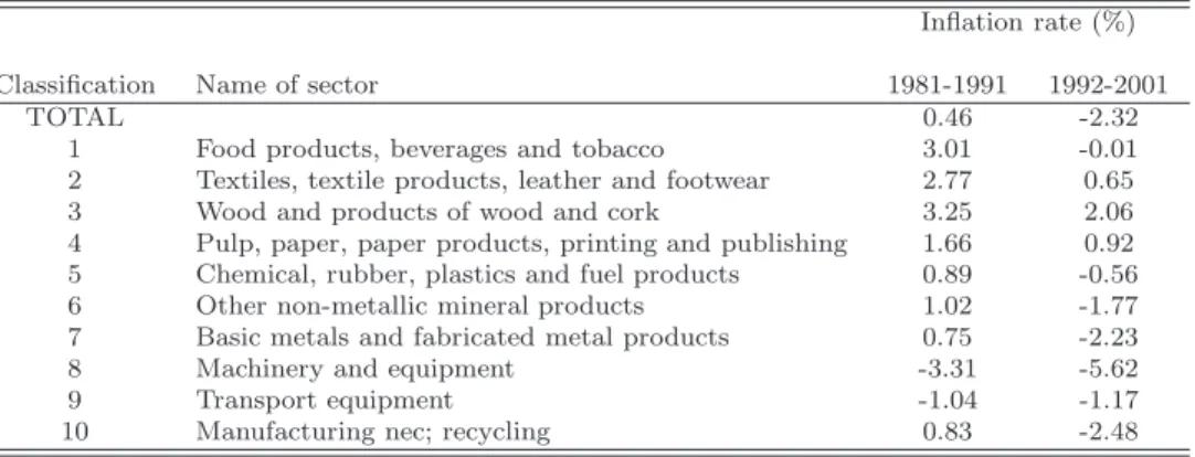
Table 1: Inflation rates in 10 manufacturing sectors (1981-2001)
Inflation rate (%) Classification Name of sector 1981-1991 1992-2001
TOTAL 0.46 -2.32
1 Food products, beverages and tobacco 3.01 -0.01 2 Textiles, textile products, leather and footwear 2.77 0.65 3 Wood and products of wood and cork 3.25 2.06 4 Pulp, paper, paper products, printing and publishing 1.66 0.92 5 Chemical, rubber, plastics and fuel products 0.89 -0.56 6 Other non-metallic mineral products 1.02 -1.77 7 Basic metals and fabricated metal products 0.75 -2.23
8 Machinery and equipment -3.31 -5.62
9 Transport equipment -1.04 -1.17
10 Manufacturing nec; recycling 0.83 -2.48
Table 2: Descriptive statistics of the explanatory variables
Productivity
growth (%) Index of regulation ofthe market
Import penetration rate (%) Sector 1981-1991 1992-2001 1981-1991 1992-2001 1981-1991 1992-2001 TOTAL 4.00 3.18 0.22 0.22 6.14 10.07 1 -0.62 -0.25 0.93 0.90 7.64 10.26 2 1.96 -0.7 0.01 0.00 10.6 24.79 3 2.68 -2.32 0.00 0.00 12.1 21.26 4 3.04 0.44 0.00 0.00 2.51 2.67 5 3.45 2.65 0.58 0.64 9.27 9.30 6 3.44 1.60 0.05 0.07 1.81 3.40 7 3.28 0.91 0.07 0.07 4.80 5.03 8 8.71 6.29 0.30 0.24 4.61 11.32 9 4.39 2.64 0.14 0.13 3.36 5.19 10 3.53 1.60 0.11 0.17 4.72 7.52
Vacancy rate (%) Disputes by establishment (%) Share of part-time workers (%) Sector 1981-1991 1992-2001 1981-1991 1992-2001 1981-1991 1992-2001 TOTAL 3.28 1.66 0.94 0.51 15.6 18.60 1 3.01 1.88 0.08 0.03 29.73 37.84 2 5.29 2.85 0.14 0.20 22.66 26.58 3 3.39 2.32 0.04 0.05 13.52 14.29 4 2.64 1.64 0.33 0.24 13.96 16.3 5 2.24 1.18 0.25 0.07 10.95 14.73 6 2.98 1.22 0.17 0.07 10.60 12.32 7 4.00 1.89 0.10 0.04 10.08 11.99 8 3.42 1.41 0.22 0.08 14.05 14.36 9 2.47 1.00 0.26 0.11 8.48 11.63 10 3.37 1.23 0.06 0.03 22.33 24.40
Table 3: Results of the linear estimation
Price index of value added Linear model Productivity −0.691⋆⋆⋆ (−19.1) Imports −0.070⋆⋆⋆ (−2.76) Regulation 0.496⋆⋆⋆ (3.39) Vacancy rate 0.029⋆⋆⋆ (4.71) Disputes 0.038⋆⋆ (2.90) Part-time −0.109⋆⋆ (−2.22) M2 0.447⋆⋆⋆ (15.6)
Notes: Following the results of the Hausman test, this specification is estimated with random individual effects. t-statistics are in parenthe-ses. ***: significant at the 1% level; **: significant at the 5% level; *: significant at the 10% level.
Table 4: Tests of linearity
Threshold variable Productivity Import Part-Time Disputes Vacancy Rate Linearity test 86.17 65.93 56.5 54.61 25.8 p − value 0.00 0.00 0.00 0.00 0.00 RSS 0.331 0.356 0.370 0.372 0.42
Notes: RSS denotes Sum of Squared Residuals, the p − value of the linearity test is obtained with 300 bootstrap simulations.
Table 5: Tests of linearity and determination of the number of regimes when import penetration is the threshold variable
Threshold variable Import penetration One threshold RSS 0.357 F1 65.9 p − value 0.00 Two thresholds RSS 0.293 F2 47.2 p − value 0.08 Three thresholds RSS 0.269 F3 51.7 p − value 0.00
Note: p-values are obtained with 300 bootstrap simulations.
Table 6: Four regimes panel model: Estimated parameters
Dependent variable: Price Transition: Import penetration regime Low Middle low Middle high High Productivity −0.601⋆⋆⋆ (−16.5) −0.652⋆⋆⋆ (−20.3) −0.608⋆⋆⋆ (−16.8) −0.745⋆⋆⋆ (−10.3) Regulation 0.980⋆⋆⋆ (4.52) 0.319 ⋆⋆⋆ (2.50) 0.291 ⋆⋆⋆ (2.41) −2.18⋆⋆⋆ (−3.7355) Import penetration 0.031 (1.26) −0.046(−1.35) −0.158 ⋆⋆⋆ (−3.29) −0.103 ⋆⋆⋆ (−2.40) Vacancy rate −0.016⋆⋆⋆ (−2.84) 0.045 ⋆⋆⋆ (6.10) 0.001(0.12) −0.0160 ⋆⋆ (−2.04) Disputes −0.004 (−0.36) 0.016(1.06) 0.012(0.91) 0.197 ⋆⋆⋆ (3.69) Part-time −0.139⋆⋆⋆ (−2.51) 0.035(0.60) −0.040(−0.67) −0.840 ⋆⋆⋆ (−8.40) M2 0.3535⋆⋆⋆ (12.2) 0.322 ⋆⋆⋆ (11.05) 0.366 ⋆⋆⋆ (11.3) 0.562 ⋆⋆⋆ (15.8) Threshold 1.27 1.82 2.43
Notes: t − statistics are in parentheses. ***: significant at the 1% level; **: significant at the 5% level;*: significant at the 10% level.
Figure 1: Representation of transition when import penetration is the threshold variable
0 5 10 15 20 25 1.4 1.6 1.8 2 2.2 2.4 2.6 2.8 Sector 1 0 5 10 15 20 25 1 1.5 2 2.5 3 3.5 4 Sector 2 0 5 10 15 20 25 1 1.5 2 2.5 3 3.5 Sector 3 0 5 10 15 20 25 0.8 1 1.2 1.4 1.6 1.8 2 2.2 2.4 2.6 Sector 4 0 5 10 15 20 25 1.4 1.6 1.8 2 2.2 2.4 2.6 2.8 Sector 5 0 5 10 15 20 25 −0.5 0 0.5 1 1.5 2 2.5 Sector 6 0 5 10 15 20 25 1.4 1.6 1.8 2 2.2 2.4 2.6 2.8 Sector 7 0 5 10 15 20 25 1.4 1.6 1.8 2 2.2 2.4 2.6 2.8 3 Sector 8 0 5 10 15 20 25 0.8 1 1.2 1.4 1.6 1.8 2 2.2 2.4 2.6 Sector 9 0 5 10 15 20 25 1.4 1.6 1.8 2 2.2 2.4 2.6 2.8 Sector 10
Notes: We plot the transition variable (import penetration) with respect to time and sector. The horizontal lines represent the threshold values.