HAL Id: hal-02944443
https://hal.archives-ouvertes.fr/hal-02944443
Submitted on 21 Sep 2020
HAL is a multi-disciplinary open access
archive for the deposit and dissemination of
sci-entific research documents, whether they are
pub-lished or not. The documents may come from
teaching and research institutions in France or
abroad, or from public or private research centers.
L’archive ouverte pluridisciplinaire HAL, est
destinée au dépôt et à la diffusion de documents
scientifiques de niveau recherche, publiés ou non,
émanant des établissements d’enseignement et de
recherche français ou étrangers, des laboratoires
publics ou privés.
atmospheric general circulation model on the simulation
of CO2 transport
Marine Remaud, Frederic Chevallier, Anne Cozic, Xin Lin, Philippe Bousquet
To cite this version:
Marine Remaud, Frederic Chevallier, Anne Cozic, Xin Lin, Philippe Bousquet. On the impact of
recent developments of the LMDz atmospheric general circulation model on the simulation of CO2
transport. Geoscientific Model Development, European Geosciences Union, 2018, 11 (11),
pp.4489-4513. �10.5194/gmd-11-4489-2018�. �hal-02944443�
https://doi.org/10.5194/gmd-11-4489-2018 © Author(s) 2018. This work is distributed under the Creative Commons Attribution 4.0 License.
On the impact of recent developments of the LMDz atmospheric
general circulation model on the simulation of CO
2
transport
Marine Remaud, Frédéric Chevallier, Anne Cozic, Xin Lin, and Philippe Bousquet
Laboratoire des Sciences du Climat et de l’Environnement, Orme des Merisiers, 91190 Saint-Aubin, France Correspondence: Marine Remaud (mremaud@lsce.ipsl.fr)
Received: 4 July 2018 – Discussion started: 5 July 2018
Revised: 8 October 2018 – Accepted: 16 October 2018 – Published: 9 November 2018
Abstract. The quality of the representation of greenhouse gas (GHG) transport in atmospheric general circulation mod-els (GCMs) drives the potential of inverse systems to retrieve GHG surface fluxes to a large extent. In this work, the trans-port of CO2is evaluated in the latest version of the
Labora-toire de Météorologie Dynamique (LMDz) GCM, developed for the Climate Model Intercomparison Project 6 (CMIP6) relative to the LMDz version developed for CMIP5. Several key changes have been implemented between the two ver-sions, which include a more elaborate radiative scheme, new subgrid-scale parameterizations of convective and boundary layer processes and a refined vertical resolution. We per-formed a set of simulations of LMDz with different phys-ical parameterizations, two different horizontal resolutions and different land surface schemes, in order to test the impact of those different configurations on the overall transport sim-ulation. By modulating the intensity of vertical mixing, the physical parameterizations control the interhemispheric gra-dient and the amplitude of the seasonal cycle in the Northern Hemisphere, as emphasized by the comparison with observa-tions at surface sites. However, the effect of the new param-eterizations depends on the region considered, with a strong impact over South America (Brazil, Amazonian forest) but a smaller impact over Europe, East Asia and North America. A finer horizontal resolution reduces the representation er-rors at observation sites near emission hotspots or along the coastlines. In comparison, the sensitivities to the land surface model and to the increased vertical resolution are marginal.
1 Introduction
The accumulation of carbon dioxide (CO2) in the atmosphere
due to anthropogenic activity is one of the primary drivers of climate change (Ciais et al., 2014a). This trace gas there-fore receives particular attention and benefits from various observation networks and systems at the surface, in the atmo-sphere and from space (e.g. Ciais et al., 2014b). These data streams can be used to locate and quantify the sources and sinks of CO2through the inversion of atmospheric transport
in a Bayesian framework. However, despite the large moni-toring effort, such estimations still suffer from large uncer-tainties (Peylin et al., 2013). For instance, atmospheric in-verse systems used in the last Global Carbon Budget of the Global Carbon Project (Le Quéré et al., 2018) disagree on the amount of the decadal land sink integrated over the northern extratropical latitudes by about 1 GtC year−1. Several factors could explain such an inconsistency, but uncertainties in the modelling of atmospheric transport have long been identi-fied as a key driver of the spread among global atmospheric inverse modelling results (Gurney et al., 2002, 2003; Basu et al., 2018).
In 1993, the Atmospheric Tracer Transport Model Inter-Comparison (TransCom) Project was created to assess the influence of different transport algorithms on the CO2
in-version problem (Law et al., 1996; Denning et al., 1999). It is still active today and has even been extended to the methane inversion problem (Patra et al., 2011). The series of TransCom and related experiments have highlighted the importance of vertical transport in this domain, with con-sequences for the strength of the seasonal rectifier of Den-ning et al. (1995), for the estimated location of the CO2sink
(Stephens et al., 2007) or for the interhemispheric exchange times (Patra et al., 2011). For instance, models simulating larger vertical gradients tend to show larger interhemispheric gradients in the lower troposphere (Krol et al., 2018; Saito et al., 2013). Actually, the quality of the simulated verti-cal transport itself is driven by various factors: horizontal and vertical resolutions, numerical diffusion, meteorological data from numerical weather prediction (NWP) centres and subgrid-scale parameterizations. Numerical diffusion arises from the grid discretization and increases with coarser res-olutions (Prather et al., 2008). Regarding horizontal resolu-tion, model intercomparison experiments showed the benefit of a refined horizontal resolution to simulate the short-term variability at continental and coastal sites (Geels et al., 2007; Law et al., 2008; Patra et al., 2008; Saeki et al., 2013; Wang et al., 2016) due to the finer description of orography and of the emission fluxes (Patra et al., 2008). However, uncer-tainties both in meteorological data and in the location of the emission hotspots limit our capacity to use higher resolution models for inversion (Lin, 2016). Even more critical are the subgrid-scale parameterizations that directly affect the simu-lated vertical gradient (Locatelli et al., 2015b).
The characteristics of global transport models for CO2
and related tracers vary widely in the atmospheric inversion community, but the models are all driven by external me-teorological data, an economy of computation which is im-portant for the simulation of the advection of a long-lived tracer like CO2, and for the computation of the associated
derivatives used in the inversion systems. The meteorolog-ical variables for these “offline” models are either directly obtained from a (higher resolution) NWP reanalysis (Olivié et al., 2004) with an appropriate interpolation procedure, or diagnosed from an NWP re-analysis (Dentener et al., 1999) or obtained from a full general circulation model (GCM) nudged to an NWP re-analysis (Hauglustaine et al., 2004). This list is ordered by increasing degrees of freedom on the model for the inverse modellers, but all three cases can provide a realistic representation of the synoptic patterns in the tracer fields. Here, we take the GCM of the Labora-toire de Météorologie Dynamique (LMDz; Hourdin et al., 2006a) that, together with its offline version, correspond to the third case, to assess the impact of the various model com-ponents on the quality of the simulation of CO2, of sulfur
hexafluoride (SF6) and of the most stable of the radon
iso-topes,222Rn. LMDz represents the atmosphere in the Earth system model of the Institute Pierre Simon Laplace (IPSL-CM, Dufresne et al., 2013) and as such has been contributing to the recent versions of the Climate Model Intercompari-son Project (CMIP) established by the World Climate Re-search Program (https://cmip.llnl.gov/, last access: 30 Octo-ber 2018). Of direct relevance for this study here is the fact that the offline version of LMDz (Hourdin et al., 2006b) as well as an associated adjoint code are used in the atmospheric inversion system of Chevallier et al. (2005), which is the cur-rent basis for the CO2inversion products of the Copernicus
Atmosphere Monitoring Service of the European Commis-sion (http://atmosphere.copernicus.eu/, last access: 30 Octo-ber 2018). At present, the offline model requires 44 times less CPU time than the corresponding full LMDz version.
The version of LMDz for the current CAMS inversion sys-tem was evaluated for the transport of tracers by Locatelli et al. (2015a) under the name LMDz5A. Compared to its previous offline version, it benefited from an increased num-ber of vertical layers from 19 to 39 and from the convective scheme of Emanuel (1991) in replacement of Tiedtke (1989). The finer vertical resolution improved the stratosphere– troposphere exchanges (STEs) that were too fast (Patra et al., 2011). The change of convective scheme increased the inter-hemispheric (IH) gradient for SF6simulations, even though
this gradient remained too weak compared to observations. As a consequence, the IH gradient in methane emissions es-timated through inverse modelling is smaller compared to the inversion based on the Tiedtke (1989) convective scheme (Locatelli et al., 2015b).
Since Locatelli et al. (2015a), new versions of the full LMDz GCM have been developed, e.g. for the ongoing CMIP6. The latter benefits from a resolution increased to 79 vertical layers and more elaborate subgrid-scale parameteri-zations in terms of convection and boundary layer processes. This version has been primarily developed for climate mod-elling and has not been tested yet for the transport of tracers such as CO2. In this context, the objectives of this paper are
twofold:
- Evaluate the effect of these new developments on the simulated values of CO2mixing ratios and, to a smaller
extent, SF6and222Rn mixing ratios, and anticipate their
benefit for inverse modelling.
- Benchmark the sensitivity of tracer transport to model set-ups. Different from a multi-model intercomparison experiment, this study provides an opportunity to focus on some model components separately.
In Sect. 2, we describe the various LMDz configurations, the observations and the analysis methods used in this study. In Sect. 3, we focus on the general behaviour of the simula-tions, considering zonal mean features and the total column of CO2. In Sect. 4, we compare the simulations with surface
and aircraft CO2measurements. Section 5 is the conclusion.
2 Data and methods 2.1 Model description
We focus here on two reference versions of LMDz that were prepared for past (fifth) and ongoing (sixth) versions of the CMIP program. In addition to different spatial resolutions, these two versions use different subgrid-scale parameteriza-tions or physics called 5A and 6A.
In the LMDz5A version (Hourdin et al., 2006a), turbu-lent transport by eddies in the boundary layer is repre-sented by a vertical diffusion scheme, in which the turbu-lent diffusion coefficient depends on the Richardson Number (Louis, 1979). A counter-gradient term on potential temper-ature (Deardorff, 1972) was added to handle dry convection cases in the boundary layer. Deep convection is parameter-ized by the episodic mixing and buoyancy sorted scheme of Emanuel (1991) in which both triggering and closure of the updraft depend on the potential convective energy available over the column (CAPE). These assumptions are based on the quasi-equilibrium (QE) hypothesis that stipulates that all convective instability available in the column is consumed instantly by deep convection that, in return, brings it back to neutral stability. The known weaknesses of this physics include the underestimation of shallow convection (Zhang et al., 2005), resulting in insufficient venting of the bound-ary layer tracers by cumulus (Locatelli et al., 2015a), the unrealistic phasing of the diurnal cycle of convection over continents, the precipitation peak being generally simulated too early in the day (Guichard et al., 2004) and the lack of tropical variability (Lin et al., 2006).
In order to address these deficiencies, a new version of the LMDz GCM, called LMDz5B, has been developed for CMIP5 (Hourdin et al., 2013). The new physics treats low and deep convection separately. On the one hand, shal-low convection is represented in a unified way by combining the diffusive approach of Mellor and Yamada (1974) for the small-scale turbulence and a mass flux scheme, the thermal plume model (Rio and Hourdin, 2008), which represents both dry and cloudy thermals in the convective boundary layer. On the other hand, deep convection and downdrafts are rep-resented by the Emanuel (1991) scheme coupled with a pa-rameterization of cold pools (Grandpeix et al., 2009). Deep convection triggering and closure are not CAPE functions anymore. They depend on sub-cloud processes. The convec-tive onset is now controlled by the thermal plume variables, and the maintenance of deep convection after its onset is op-erated by the cold pools. In better agreement with observa-tions, the main results are a delay of the convective initia-tion, a self-sustainment of convection through the afternoon (Rio and Hourdin, 2008; Rio et al., 2009) and a drastic in-crease of the tropical variability of precipitation (Hourdin et al., 2013). This version has not been implemented in the above-mentioned inversion system for CO2because
prelimi-nary CO2transport simulations showed unrealistically large
seasonal cycles at some southern stations like Palmer Station (PSA) in Antarctica (unpublished results). However, it was successfully used for aerosol data assimilation around north-ern Africa by Escribano et al. (2016) and showed promis-ing improvements for the representation of the magnitude of diurnal variations of surface concentrations (Locatelli et al., 2015a).
For CMIP6, configuration 5B of LMDz has further evolved from Hourdin et al. (2013): it has a different
formu-lation of the triggering assumptions and a different radiative transfer code, and it accounts for the thermodynamical effect of ice. The convective triggering is now based on evolving statistic properties on the thermal plumes by considering a thermal size distribution instead of a bulk thermal (Rochetin et al., 2013). The motivation behind this change was to de-part from the QE hypothesis and to allow a more gradual transition between shallow and deep convection through a three-step process (appearance of clouds, crossing of the in-hibition layer and deep convection triggering). In the short-wave, the code is an extension to 6 bands of the initial 2-band code that is used in LMDz5A (Fouquart and Bonnel, 1980), as implemented in a previous version of the European Cen-tre for Medium-Range Weather Forecasts (ECMWF) numer-ical weather prediction model. In the longwave, LMDz uses the Rapid Radiation Transfer Model (RRTM) (Mlawer et al., 1997). This version is now called 6A.
For the energy and water flux between land surface and at-mosphere, LMDz can be coupled with the ORCHIDEE (OR-ganizing Carbon and Hydrology In Dynamic Ecosystems, version 9) (Krinner et al., 2005) terrestrial model or with a simple bulk parameterization of the surface water budget.
The reference configuration of LMDz5A used in CMIP5 had 39 eta-pressure layers and 96 × 96 grid points, i.e. a hor-izontal resolution of 1.89◦in latitude and 3.75◦in longitude. Current reference simulations of IPSL-CM for CMIP6 use the new configuration of LMDz6A, with a refined grid of 144 grid points both in latitude and longitude directions and a ver-tical resolution extended to 79 layers. The number of layers under 1 km has increased from 5 to 16 layers. The remaining additional layers are mostly located in the stratosphere so that in the lower stratosphere (between 100 and 10 hPa), the ver-tical spacing 1z is approximately 1 km in this model set-up. For the inverse system, LMDz is currently run in an offline version of configuration 5A with 39 eta-pressure layers and 96 × 96 grid-points, i.e. a horizontal resolution of 1.89◦in latitude and 3.75◦in longitude.
2.2 Description of the simulations
We have run the two versions of the physics described above, 5A and 6A, at several resolutions for the years from 1988 to 2014. A summary of the simulations used is given on Table 1. The identification number of the LMDz code used here (that contains both physics versions) is 2791. We discard the first 10 years (1988–1998) to allow enough spin-up for the tracer simulations, considering the interhemispheric exchange time of about 1 year for passive tracers (Law et al., 2003). The dy-namics is nudged towards the 6-hourly horizontal winds from the ECMWF reanalysis (Dee et al., 2011) with a relaxation time of 3 h (Hourdin and Issartel, 2000). CO2, SF6and222Rn
initial values are set uniformly for all model grid boxes at a value of, respectively, 350 µmol mol−1(abbreviated as ppm), 1.95 pmol mol−1(abbreviated as ppt) and 0 Bq m−3on 1 Jan-uary 1988; 350 ppm is the global mean given for that date
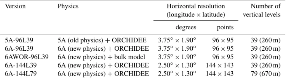
Table 1. Description of the simulations. The vertical spacing averaged over the tropics (between the surface and 10 km) is indicated in brackets.
Version Physics Horizontal resolution Number of
(longitude × latitude) vertical levels
degrees points
5A-96L39 5A (old physics) + ORCHIDEE 3.75◦×1.90◦ 96 × 95 39 (260 m)
6A-96L39 6A (new physics) + ORCHIDEE 3.75◦×1.90◦ 96 × 95 39 (260 m)
6AWOR-96L39 6A (new physics) + bulk model 3.75◦×1.90◦ 96 × 95 39 (260 m)
6A-144L39 6A (new physics) + ORCHIDEE 2.50◦×1.30◦ 144 × 143 39 (260 m)
6A-144L79 6A (new physics) + ORCHIDEE 2.50◦×1.30◦ 144 × 143 79 (670 m)
by the forward simulation associated with the CAMS CO2
inversion used here (see Sect. 2.3) and 1.95 ppt is the ini-tial value used for SF6in the TransCom protocol of Denning
et al. (1999). The initial value of222Rn does not matter given the short lifetime of this radionuclide. The time step of model output is hourly.
Numerical approximations in the advection scheme and in the subgrid parameterizations prevent LMDz from strictly conserving mass. For CO2, for instance, the model loses
about 1 GtC integrated over 10 years in the reference version and twice as much in the new version. We have therefore ap-plied a global mass correction both on the CO2and the SF6
3-D mole fraction fields every hour. The correction method consists in a diagnostic of the loss at each timestep which is then added back, evenly distributed through space.
2.3 Prescribed tracer fluxes at the surface
CO2 surface fluxes are prescribed every 3 h from version
15r4 of the CO2atmospheric inversion product of the CAMS.
The 3-hourly resolution is allowed by prior information to the inversion system, while surface air sample measurements constrained the fluxes at weekly or coarser resolution (they also correct a mean day–night difference every day but this is marginal). The inversion system assimilated the surface measurements for the period 1979–2015 in an offline ver-sion of LMDz5A at a horizontal resolution of 3.75◦×1.90◦ (longitude × latitude). Of interest here is the use of fossil fuel emissions from the Emission Database for Global At-mospheric Research version 4.2 (EDGAR, http://edgar.jrc. ec.europa.eu/, last access: 30 October 2018) scaled to the an-nual global values of the Global Carbon Project (Le Quéré et al., 2015). Details of the prescribed fluxes are given in Chevallier (2017). As a consequence, the surface fluxes carry some imprint of a version of LMDz close, but not identical, to 5A-96L39. Fluxes from another atmospheric inversion could have been used instead, but recall that the most robust atmo-spheric inversions share the same surface measurements to a large extent, so that the question of the lack of independence of our CO2simulations to the surface measurements would
remain anyway. In the Supplement, we show the robustness of our conclusions with respect to a change of the CO2
sur-face fluxes from CAMS to CarbonTracker (https://www.esrl. noaa.gov/gmd/ccgg/carbontracker/, last access: 30 October 2018).
For use at a resolution of 2.50◦×1.30◦, the natural com-ponent of the optimized fluxes has been interpolated from its native 3.75◦×1.90◦ resolution, and has been completed by a fossil fuel component directly interpolated from the EDGAR native 0.1◦×0.1◦ resolution in order to avoid ar-tificial smoothing. All grid changes here conserve mass.
Monthly averages of SF6 emission fluxes at 1◦×1◦ are
taken from the EDGAR 4.0 inventory for the period 1988– 2008 as corrected by Levin et al. (2010). The global emis-sions steadily increased from 934 mmol s−1 in 1988 to 1599 mmol s−1in 2010. Since these sources are mostly in the Northern Hemisphere and since there are no sinks, SF6has
been largely used to gain further insight into IH transport and STEs. We additionally prescribe222Rn surface fluxes accord-ing to Patra et al. (2011). With its short lifetime (3.8 days),
222Rn is used here to gain some insight into the vertical
mix-ing within the column.
2.4 Observations and data sampling 2.4.1 Model sampling strategy
For each species, the simulated concentration fields were sampled at the 3-D grid boxes nearest to the observation lo-cation. They were also sampled to the nearest hours from the time when the observations were taken. Observations are all dry air mole fraction measurements calibrated relative to the CO2World Meteorological Organization (WMO) mole
frac-tion scale. For comparison, the corresponding dry air vari-ables in the model simulations are used. In Sect. 3, even though the model simulations are not compared to measure-ments, the model sampling still refers to some observation selection (in the afternoon for the zonal mean profiles, or fol-lowing a satellite retrieval pattern for the total column), as indicated in the corresponding text.
Figure 1. CO2 sampling locations. Red dots denote the subset of the assimilated site locations that are used here. Yellow dots denote
unassimilated site locations. Blue dots denote independent aircraft measurement locations in North and South America (other aircraft sites for the rest of the world are shown in Fig. 2). Specific areas for our study are shown in red: Europe (EUR: 40–70◦N, 10◦W–50◦E), greater northern India (IND: 20–30◦N, 70–100◦E), East Asia (EAS: 20–50◦N, 100–150◦E) and northern Southeast Asia (NSA: 10–20◦N, 90– 160◦E). Stations RPB and ASC, in black even though they have been assimilated, are the NOAA tropical Atlantic sites used to define the background concentrations of CO2and SF6coming into the Amazon basin.
2.4.2 Point samples from surface sites
The surface measurements of SF6 are taken at background
stations SPO, PSA, CGO, SMO, RPB, MLO, MHD, BRW, SUM and ALT from the NOAA/ESRL network (http://www. esrl.noaa.gov/gmd, NOAA ESRL GMD, 2015).
The simulated mole fractions of CO2were compared with
some of the atmospheric surface measurements that were assimilated when optimizing the surface CO2 fluxes
pre-scribed here. The location of these assimilated surface sta-tions is shown in Fig. 1. As in the CAMS inverse modelling framework, we only retain early afternoon data (12:00– 15:00 LST) for continuous stations under 1000 m a.s.l. and night-time data (00:00–3:00 LST) for continuous station above 1000 m a.s.l. All measurements from flasks below 1000 m a.s.l. have been kept. The reasons behind this hour selection are the failure of transport models in general to ac-curately represent the accumulation of tracers near the sur-face at night and the advection of air masses during the day by upslope winds over sunlit slopes in the afternoon (Geels et al., 2007). A description of the surface observations used for the inversion can be found in Chevallier (2017), but only a subset is used here. This subset comes from the obspack_co2_1_GLOBALVIEWplus_v3.2_2017-11-02 archive (Cooperative Global Atmospheric Data Integration Project, 2017), from the World Data Center for Green-house Gases archive (https://ds.data.jma.go.jp/gmd/wdcgg/, last access: 30 October 2018) and from the Réseau Atmo-sphérique de Mesure des Composés à Effet de Serre monitor-ing network (https://www.lsce.ipsl.fr/, last access: 30 Octo-ber 2018). We have selected the sites with more than 3 years
Figure 2. Number of CONTRAIL measurements used here at 5.5 km above sea level, within the model grid boxes (3.75◦×1.90◦). The specific areas of Fig. 1 are also shown. Prior to the calculation of this number, the measurements were averaged hourly in each grid box.
of record and with enough data density in time to compute the statistics.
In addition, we use some unassimilated surface observa-tions in the tropics (bkt, cri, hkg, hko, lln and hat – note the lower case used here to denote sites unassimilated in the Chevallier, 2017 inversion) to better evaluate the quality of the inversion over the tropics which are not well constrained. We sampled the model output at the elevation (above sea level) corresponding to the actual elevation of each site. The hkg and hko observations only provide the daily mean mole fraction of CO2.
2.4.3 Vertical profile samples from aircraft measurements
We have compared the simulated CO2mole fractions against
observations of CO2 vertical profiles from three sampling
programs: Comprehensive Observation Network for TRace gases by AIrLiner (CONTRAIL), the NOAA/ESRL Global Greenhouse Gas Reference Network Aircraft Program and the lower tropospheric greenhouse gases sampling program over the Amazon described in Gatti et al. (2014). Aircraft measurements have not been assimilated in the CAMS in-version product and are therefore called independent in the following.
CONTRAIL (Machida et al., 2008, http://www.cger. nies.go.jp/contrail/index.html) provides high-frequency CO2
measurements over 43 airports worldwide and during com-mercial air flights between Japan and other countries. The calibration of the data is assured within 0.2 ppm (Machida et al., 2008). We selected from the CONTRAIL dataset all the CO2vertical profiles during the ascending and
descend-ing flights for the period 2006–2011 over the regions por-trayed in Fig. 1. The regions are similar to Niwa et al. (2011) and have been chosen according to the number and location of the vertical profile samples. The number of hourly mean measurements at 5.5 km a.s.l. per model grid box are shown in Fig. 2 considering a model resolution of 3.75◦×1.90◦. There are 862 hourly mean vertical profiles over EUR, 4124 over EAS, 265 over NSA and 153 over IND.
The NOAA/ESRL Global Greenhouse Gas Reference Net-work Aircraft Program consists here of measurements of air samples collected every few days or months at 22 aircraft profiling sites over continental North America (shown in blue in Fig. 1) between altitudes of 300 and 8000 m a.s.l. In the lowest altitudes, compared to the CONTRAIL measurements that have been sampled at nearby commercial airports, these measurements are not affected by local emissions. We per-formed statistics on 974 available vertical profiles.
The lower tropospheric greenhouse base sampling pro-gram over the Amazon provides biweekly air sample profiles from above the forest canopy (300 m) to 4.4 km above sea level at four sites (san, tab, alf and rba) in 2010. The loca-tions of the airborne platforms are shown in blue in Fig. 1. During their descending flights, small aircrafts filled flasks between 12:00 and 13:00 LST when the boundary layer is fully developed. Most of the samples are representative of air masses that have been blown away by the dominant east-erly flow from the tropical Atlantic Ocean across the Ama-zonian basin. Air masses at sites tab and rba are mainly re-lated to transport of source and sinks from a large fraction of the Amazonian forest. Air masses at Alta Floresta (alf) and Santarem (san) are related to transport of sources and sinks of savanna and agricultural lands within their footprint areas. These aircraft data are fully described in Gatti et al. (2014) and are available at ftp://ftppub.ipen.br/nature-gatti-etal/.
2.5 Post-processing of the CO2simulations and
measurements
In Sect. 4, the features of interest (annual mean, monthly smooth seasonal cycle, synoptic variations) are derived from the surface data using the CCGVU curve fitting procedure developed by Thoning et al. (1989) (Carbon Cycle Group Earth System Research Laboratory (CCG/ESRL), NOAA, USA) and following the set-up of Lin et al. (2017). The CCGVU procedure is fully described and freely available at http://www.esrl.noaa.gov/gmd/ccgg/mbl/crvfit/crvfit.html. The procedure estimates a smooth function by fitting the CO2
time series to a first-order polynomial equation for the growth rate combined with a two-harmonic function for the annual cycle. The seasonal cycle and annual gradient are extracted from the smooth function while the synoptic variability is de-fined from a residual time series between the smooth function and the raw time series. In addition, outliers are discarded if their values exceed 3 times the standard deviation of the residual time series.
For each station, the annual gradient to MLO is calcu-lated by subtracting the annual mean of the CO2mole
frac-tion at MLO (Mauna Loa, 19◦520N 155◦580W) from the annual mean from the smooth curve of the station of inter-est. Regarding the seasonal cycle, the amplitude is calcu-lated from the smooth curve as an absolute peak-to-peak dif-ference within a year at each site. Then, we average these yearly amplitudes over the period 1998–2014. The seasonal phase is evaluated using the Pearson coefficient between ob-served and simulated smooth curves. The synoptic curve is extracted at each site from the residual between the raw time series and the smooth curve. In order to plot the sea-sonal latitudinal gradient of CO2, we choose marine
bound-ary layer sites: ZEP (Zeppelin, Ny-Ålesund, Svalbard, Nor-way and Sweden), ICE (Storhofdi, Vestmannaeyjar, Iceland), SHM (Shemya Island, Alaska, USA), AZR (Terceira Island, Azores, Portugal), MID (Sand Island, Midway, USA), MNM (Minamitorishima, Japan), KUM (Cape Kumukahi, Hawaii, USA), GMI (Mariana Islands, Guam), CHR (Christmas Is-land, Republic of Kiribati), SMO (Tutuila, American Samoa) and CGO (Cape Grim, Tasmania, Australia).
The synoptic variability is evaluated using two quanti-ties: the Pearson correlation coefficient and the model-to-observations ratio of the standard deviation (normalized stan-dard deviation, NSD) between the observed and simulated residual time series. For each site, the diurnal amplitude is calculated from a residual time series between the raw time series of the CO2mole fraction and its daily mean.
For the airborne measurements from the NOAA/ESRL Global Greenhouse Gas Reference Network and from CON-TRAIL, only the CO2 samples taken in the afternoon
(be-tween 11:00 and 20:00 LST) have been retained. The result-ing samples have been averaged into vertical bins of 1 km for each hour, before being averaged spatially for a given region of Fig. 1 and monthly. For each subregion and each 1 km
al-titude bin, a detrended signal at 3.5 km has been subtracted from the time series. Over the Amazon, a background time series has been subtracted from the simulated and observed vertical profiles using the same method described in Gatti et al. (2014).
3 General behaviour 3.1 Zonal mean structures
We first study the zonal mean structure of the 222Rn, SF6
and CO2simulations. We focus on the boreal summer (JJA)
as the convection is more active over Northern Hemisphere continents during this season and the spread among the ver-sions is the largest. Figure 3a shows the vertical structure of the zonal mean mole fraction of 222Rn from 5A. 222Rn is a short-lived radioactive tracer naturally emitted by con-tinental surfaces that decays radioactively with a half time of 3.8 days. Its lifetime is comparable to that of mesoscale convective systems over the tropics (10 h on average but it can reach 2–3 days; Houze, 2003). For this reason,222Rn has been largely used by modellers to evaluate vertical transport operated by subgrid-scale processes in the planetary bound-ary layer (PBL) and lower troposphere (Genthon and Ar-mengaud, 1995; Belikov et al., 2013). The vertical profile, with a maximum at ground level and a decrease with in-creasing height, mainly reflects the transport by convective processes between 10 and 70◦N from the boundary layer to the tropopause.
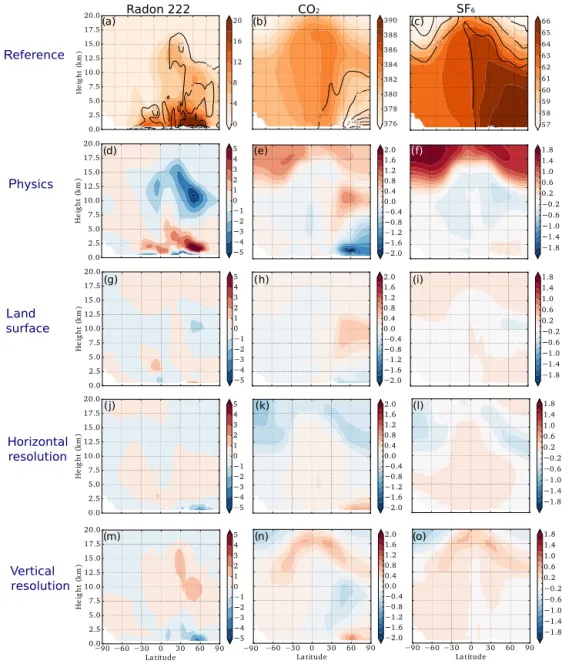
Figure 3d shows that the effect of the modified physics is a radon depletion with respect to 5A over the entire mid-troposphere above 7.5 km, between 30◦S and 80◦N. The largest relative depletion, of about half of the 222Rn con-centrations in 5A, occurs in the northern mid-latitude tro-posphere around 10 km. The lower concentrations of 222Rn suggests that there is, on average, less convection penetrating into the upper troposphere in the new physics. However, the increase of 222Rn at 2.5 km and the decrease at the surface manifests from the thermal activity that transports tracers from the surface to the top of the boundary layer. The mean reduction in active convection over the continents shown by the222Rn mole fraction suggests that an effect of the stochas-tic triggering based on thermal activities is to prevent the trig-gering of spurious deep convection. This observation is con-sistent with previous findings that thermal activities reduce the strength of the deep convection (Rio et al., 2009; Locatelli et al., 2015a). The land surface model (Fig. 3g), the horizon-tal resolution (Fig. 3j) and the vertical resolution (Fig. 3m) have a modest effect on the vertical structure of222Rn com-pared to the physics. They enhance (land–surface) or atten-uate (vertical resolution) the changes induced by the new physics in the northern mid-latitudes. For instance, Fig. 3m shows a slight increase around 10 km (10 % of the total
con-centration), meaning that more deep convection penetrates within the upper troposphere with a finer vertical resolution. SF6 is a quasi-inert gas released into the atmosphere by
electrical and metal industries (Maiss et al., 1996). Because of its quasi-inert nature (lifetime around 1000 years; Ravis-hankara et al., 1993; Morris et al., 1995; Kovács et al., 2017; Ray et al., 2017) and its weak seasonality, we use SF6 to
gain insight into the large-scale transport in our simulations. Figure 3f, i, l and o highlight the effects of the model set-ups described earlier on the zonal mean distribution of SF6.
The modified subgrid-scale parameterization has much more impact on the zonal mean of SF6 in the stratosphere than
in the troposphere. The stratosphere is not as mixed as the troposphere, resulting in a longer exchange timescale and in an integration of the differences over time. The higher mole fraction of SF6means the air is younger, suggesting an
accel-erated Brewer–Dobson circulation. The effect of the physical parameterizations on the STE fluxes has also been noticed by Hsu and Prather (2014), using two cycle versions (with two physics) of the ECMWF fields as an input to their offline transport model. The cause of this modified stratospheric dy-namics is unclear and requires further investigation. Out of the stratosphere, differences between simulations are, on the whole, small. By comparison, they are within the compatibil-ity range of 0.02 ppt recommended by the WMO for the sur-face measurements from different laboratories (Global At-mosphere Watch, 2015). The negative anomaly at 10 km is an exception. It reaches −0.06 ppt in Fig. 3f in the northern mid-latitudes, consistent with a less efficient vertical mixing induced by the new physics. In the Northern Hemisphere, the positive anomaly of 0.02 ppt in the boundary layer reveals an increase both of the surface latitudinal gradient and of IH ex-changes. The strength of the latitudinal gradient of SF6is a
good indicator of IH exchange as emissions are mainly lo-cated in the Northern Hemisphere. The increase of the latitu-dinal gradient along with a weaker vertical mixing are consis-tent with Krol et al. (2018), who showed that the IH transport timescale is negatively correlated with the efficiency of ver-tical mixing and, hence, to the parameterization of subgrid-scale processes.
Contrary to SF6, the zonal mean distribution of CO2
ex-hibits a strong seasonality in the northern mid-latitudes. In boreal winter, the prevalence of the fossil fuel emissions along with stable boundary layer conditions contribute to an increase in CO2 in the boundary layer. In boreal summer,
the CO2sink by photosynthesis outweighs fossil fuel
emis-sions and terrestrial sources (respiration, land use), leading to a net drawdown of CO2 mole fraction at the surface as
seen in Fig. 3b beyond 50◦N. As a result, the effect of the physics has an opposite sign on the CO2distribution
com-pared to SF6: a negative anomaly greater than 1.5 ppm in the
PBL and a positive anomaly of 0.5 ppm around 10 km. The new physics amplifies the trapping of negative anomalies of CO2 near the surface, consistent with a less efficient
Figure 3. Zonal mean mole fraction of (a)222Rn in 1021mol mol−1, (b) CO2in ppm and (c) SF6in 0.1 ppt from 5A-96L39. The standard
deviation is superimposed with contour lines. (d–f) Zonal mean mole fraction difference between 6A-96L39 and 5A-96L39 (effect of the new physics). (g–i) As (d–f) but between 6A-96L39 and 6AWOR-96L39 (effect of the land surface model ORCHIDEE). (j–f) As (d–f) but between 6A-144L39 and 6A-96L39 (effect of the horizontal resolution). (g–i) As (d–f) but between 6A-144L79 and 6A-144L39 (effect of the vertical resolution). The zonal mean is calculated for afternoon hours from 2005 to 2010 in summer (JJA).
Brewer–Dobson circulation induced by the new physics re-sults in an increase of 1 ppm, which represents about one-quarter of the seasonal variability of CO2 between 16 and
17 km (Diallo et al., 2017). The land surface and resolution have a modest impact on the vertical distribution of CO2.
3.2 Simulated xCO2convolved with the OCO-2
space–time coverage
In a similar way to the zonal mean distribution, we analyse the seasonal climatology of the column-average dry air mole
fraction of CO2, denoted xCO2, convolved with the space–
time coverage of NASA’s retrievals from the Second Orbit-ing Carbon Observatory (OCO-2; ElderOrbit-ing et al., 2017). We used all retrievals for the year 2017 from version 8r that are flagged as “good” by this algorithm (O’Dell et al., 2012). Figure 4 shows that the physics has the strongest impact on the annual and seasonal climatology of xCO2 fields. In
bo-real winter, the differences between the two physics exceed 0.5 ppm over tropical South America and tropical southern Africa. In boreal summer, the differences are negative and exceed 0.3 ppm in terms of absolute value beyond 50◦N.
(a) (d) (b) (d) (e) (g) (f) (h)
Figure 4. Map of the differences in xCO2 (ppm) between 6A-96L39 and 5A-96L39 (a, b, effect of the new physics), 6A-96-L39 and
6AWOR-96L39 (c, d, effect of the land surface), 6A-144L39 and 6A-96L39 (e, f, effect of the horizontal resolution) and 6A-144L79 and 6A-144L39 (g, h, effect of the vertical resolution). The left column shows the average over the 2005–2010 boreal winters (December– February), and the right column shows the average over 2005–2010 boreal summers (June–August). The simulated xCO2values have been
temporally convolved with the sampling of the OCO-2 satellite retrievals for the year 2017.
This is due to the weaker vertical mixing of the new physics which limits IH exchanges: the negative anomalies of xCO2
are more trapped in the Northern Hemisphere. Compared to the physics, the land surface scheme and the horizontal and vertical resolutions have a modest effect on xCO2, with
most differences less than 0.3 ppm. The values of 0.3 and 0.5 ppm mentioned here refer to, respectively, the thresh-old and breakthrough requirements for systematic errors in satellite retrievals as defined in the User Requirement Doc-ument of ESA’s Greenhouse Gas Climate Change Initiative project (GHG-CCI, 2016). Comparing model performance to retrieval requirements is motivated by the same role that
model errors and retrieval errors play in atmospheric inver-sions. In our case, 6 % of the winter land grid points and 5 % of the summer land grid points exceed the 0.5 ppm min-imum requirement in terms of the differences between the two physics.
If the horizontal resolution has a modest effect on the xCO2values at a large scale, its impact can be much larger
at a local scale and exceed 0.5 ppm in individual grid points. The impact of the horizontal resolution is particularly notice-able over northern India. In comparison, the effect of the land surface scheme and of the vertical resolution are modest.
o o o o o o o o o o
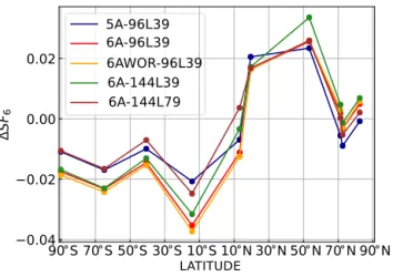
Figure 5. Latitudinal distribution of the SF6bias (modelled –
ob-served) at the surface background stations during years 2005–2009. The stations used are: SPO, PSA, CGO, SMO, RPB, MLO, MHD, BRW, SUM, ALT.
4 Comparison with observations 4.1 Interhemispheric gradient with SF6
A classical approach to evaluate the intensity of the IH ex-changes is to plot the latitudinal distribution of the SF6mole
fraction at the surface (Denning et al., 1999). The 5-year mean of the model-minus-observation mole fraction differ-ence at the 11 background surface stations, in Fig. 5, sug-gests that the IH exchanges are not sufficient in all ver-sions as the gradient is systematically overestimated. The model spread has a value of 0.01 ppt for all latitudes, re-maining smaller than the ensemble absolute bias of about 0.02 ppt. Both the ensemble spread and the ensemble bias usually remain smaller, by comparison, to the measurement calibration uncertainty of 0.03 ppt (96 % confidence interval; NOAA ESRL GMD, 2015). The consistent negative differ-ence of 0.01 ppt in the Southern Hemisphere induced by the new physics increases the surface latitudinal gradient and re-lates to the weaker vertical mixing. The vertical resolution cancels the effect of the physics by decreasing the latitudinal gradient and even improves it slightly.
4.2 Impact of the model set-ups on the CO2-simulated
concentrations at the surface and in the mid-troposphere
We now quantify the sensitivity of the simulated surface val-ues of CO2to the model set-ups at annual, seasonal, synoptic
and diurnal scales. From this perspective, we quantify the model spread of the simulated mole fraction for each surface site (total of 65 sites) that have been used for optimizing the prescribed fluxes during the years 1998–2014. Since the CO2
fluxes have been estimated from a model version close to 5A-96L39, the best match between model and observations
Table 2. Simulated mean gradients of CO2mixing ratios between MLO and other stations located in the Northern Hemisphere (lat-itudes > 30◦N), the tropics (30◦S ≤ latitudes ≤ 30◦N) and the Southern Hemisphere (latitudes < 30◦S). For each one of the three domains, the corresponding sites are weighted by the inverse of their standard deviation. The value inside the brackets defines the associ-ated mean weighted standard deviation.
Version Northern Tropics Southern
Hemisphere Hemisphere 5A-96L39 1.7 (0.1) −0.4 (0.1) −3.0 (0.1) 6A-96L39 1.7 (0.1) −0.4 (0.1) −2.8 (0.1) 6AWOR-96-L39 1.5 (0.1) −0.2 (0.1) −3.0 (0.1) 6A-144L39 1.4 (0.1) −0.3 (0.1) −3.0 (0.1) 6A-144L79 1.6 (0.1) −0.4 (0.1) −2.8 (0.1)
is expected to be obtained with this version. This is not nec-essarily true for the synoptic and diurnal scales, which have not been constrained by inverse modelling. The location of the sites is depicted in Fig. 1.
We also assess the ability of the different versions to repre-sent unassimilated observations at surface sites located over the tropics. In the prescribed surface fluxes, the tropics repre-sent 1.6 ± 0.9 Pg C year−1of the 4.3 Pg C year−1global total flux averaged for the years 2004–2011. Despite its impor-tance, this part of the globe is not well constrained by inverse modelling systems (Peylin et al., 2013).
Last, we briefly look at the quality of the model simula-tions between 5 and 6 km above sea level by comparison to aircraft measurements. Aircraft measurements will be more extensively used in Sect. 4.3 in terms of profiles.
4.2.1 Annual surface gradient to MLO
The annual gradient between stations reflects both large-scale transport and integrated fluxes over large areas. Table 2 shows the mean and standard deviation of the annual gradient of the stations in the Northern Hemisphere, in the tropics and in the Southern Hemisphere, to MLO. On average over these latitudinal bands, the differences among simulations do not exceed 0.3 ppm and remain in the range of the measurement calibration objective defined by the WMO. A total of 10 con-tinental or coastal stations out of 65 assimilated surface sites (BRW, SHM, KAS, HUN, UTA, AMY, PAL, WLG, LEF, MHD) show differences larger than 0.3 ppm.
We performed the same analysis with a regional grouping of the stations, using the tiling of the globe in 22 regions de-fined by the TransCom 3 protocol (Gurney et al., 2002). The largest systematic difference among the simulations is found for the boreal North America region (0.4 ppm), where the standard mean deviation around the annual mean is roughly 0.3 ppm for each simulation. In this case, boreal North Amer-ica is only represented by the inland site BRW, which may not be representative of the whole region.
Figure 6. (a) Correlations between the observed and simulated CO2mean seasonal cycles from 6A-96L39 (x axis) and 5A-96L39 (y axis) for all available stations. (b–d) Same as (a) but from versions 6AWOR-96L39, 6A-144L39, 6A-144L79. (e) Ratio of the simulated to observed CO2seasonal amplitude from 6A-96L39 (x axis) and 5A-96L39 (y axis) for all available stations. (f) Same as (a) but from 6A-96L39 (x axis)
and 6AWOR-96L39 (y axis). (g) Same as (f) but from 6A-96L39 (x axis) and 6A-144L39 (y axis). (h) Same as (f) but from 6A-144L39 (y axis) and 6A-144L79 (x axis). The stations are numbered by increasing latitude (with the identifier correspondence given in the bottom of the panel) and are coloured according to their category. Blue: maritime stations, black: mountainous stations, yellow: coastal station, brown: continental station. Stations written in lowercase (uppercase) refer to unassimilated (assimilated) stations.
4.2.2 Seasonal variability
The impact of the model set-ups on the seasonal cycle at each station is documented considering two characteristics: the phase and the amplitude. The ratio of simulated to ob-served amplitude of the seasonal cycle is depicted for each station in Fig. 6e–h, while the phase is displayed in Fig. 6a–d. For comparison purposes, the amplitude and phase are plot-ted separately for two versions simultaneously.
Regarding the phase (panels a–d), most station points are located close to the bisector. This means that the phase is well captured (correlation above 0.9) and is not affected much by the model set-ups for most of the assimilated stations, includ-ing for station PSA (ratio of 1.1 and correlation of 0.99 with 6A-96L39) that was not well simulated by the previous in-termediate version, 6A (see Sect. 2.1). However, the seasonal features of the unassimilated stations (lln, hat, dmv, hkg, hko, cri) appear to be much more sensitive to the model set-ups,
especially to the resolution. Station dmv is not depicted here since the correlation coefficient is less than 0.3 and the ampli-tude ranges between 0.3 and 0.6 depending on the model set-up. The poor representation of the seasonal cycle of dmv has already been noticed by Lin et al. (2017). They attributed this deficiency to inaccurate prior net ecosystem exchange (NEE) and/or fire emissions in the prescribed surface fluxes as the CH4 seasonal cycle was in better agreement with
observa-tions compared to the CO2-simulated values in their model.
This explanation is likely, given that the region is poorly con-strained by observations. Because of their strong sensitivity to the model set-ups, these stations should be associated with a strong error if they are assimilated in the inverse system, which explains why they have been discarded so far from the inversion system. The new physics increases the seasonal amplitude at (assimilated) mid-latitude sites over land: 9 sta-tions out of 26 have an amplitude shift larger than or equal to
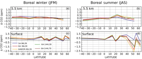
Figure 7. Latitudinal mean distribution of the CO2 bias (modelled – observed) between 5 and 6 km above sea level in the free tropo-sphere (a, b) and at the marine boundary layer (MBL) sites (c, d) for January–February–March (JFM) (a, c) and July–August–September (JAS) (b, d) during the period 2007–2010. The MBL sites are ZEP, ICE, SHM, AZR, MID, MNM, KUM, GMI, SMO, CGO. The 5–6 km measurements come from the CONTRAIL database.
0.2 ppm as a result of the convective inhibition. The horizon-tal resolution has an impact limited to only three assimilated stations, that show an amplitude shift larger than or equal to 0.2 ppm. This is due to a change of topography and land frac-tion map. The amplitude at most mountain stafrac-tions (seven) is underestimated by more than 0.1 ppm in all versions even though they have been assimilated.
Figure 7 depicts the seasonal mean latitudinal structure of the CO2bias (modelled minus observed) at marine surface
sites and at 5.5 km in boreal winter (JFM) and in boreal sum-mer (JAS). In winter, the model spread reaches a value larger than 0.5 ppm both at the surface and at 5.5 km. In summer, the model spread reaches a value of 1.5 ppm near the surface beyond 40◦N, mainly due to the physics. Consistent with a less efficient mixing inferred in the zonal mean structure (Fig. 3), the new physics decreases (increases) the latitudi-nal gradient in boreal mid-latitudes in summer at the surface (at 5.5 km) as the negative anomalies are more trapped in the boundary layer. For all simulations, the latitudinal gradient at 5.5 km between 50◦N and 40◦S is well reproduced as the bias does not exceed 0.5 ppm.
4.2.3 Synoptic variability at the surface
The synoptic variability characteristics, normalized standard deviation (NSD) and correlations with observations, are de-picted for each station in Taylor diagrams in Fig. 8. NSD refers to the ratio of the simulated to observed standard devi-ation. Consistent with the design of Taylor diagrams, the dis-tance between an actual model result and the reference (the star) is equal to the relative root mean square error. Unsur-prisingly, the model-minus-observation mismatch is not as good as for the seasonal variability. Indeed, the synoptic scale has not been constrained by the inverse modelling system. In the reference version, most stations (58 out of 72) have
cor-relations around 0.8 and an NSD around 0.7. The lack of syn-optic variability in 5A-96L39 has been reported over Europe (Locatelli et al., 2013) and over Asia (Lin et al., 2017). All versions of the model have difficulties in accurately repro-ducing the synoptic variability at the mountain stations. The new physics enhances the standard deviation at some sites lo-cated in the northern mid-latitudes. The horizontal resolution has a mixed impact: it slightly increases the amplitude but in-creases or dein-creases the correlation coefficient depending on the sites. This can be attributed to the coarse resolution of the prescribed fluxes or to NWP forcing uncertainties. The syn-optic variability is not affected by the land surface scheme nor by the vertical resolution. As for the seasonal variability, the improved horizontal resolution has a limited impact on the simulated synoptic variability to only three assimilated sites (KZM: 45, CHL: 64, HUN: 52) in terms of amplitude and correlations with observations. All versions poorly sim-ulate synoptic variability at site hko since the site is located in an urban area and is affected by local emissions not well described in the prescribed surface fluxes.
4.2.4 Diurnal cycle at the surface
The simulated CO2 diurnal variation reflects the day–night
contrast in both the prescribed fluxes and the PBL (plane-tary boundary layer) vertical mixing. Since the fossil fuel emission inventory is constant here within a month, most of the diurnal variability comes from the prior biospheric fluxes, with marginal corrections having been brought by the inverse modelling system. Another part of the diurnal vari-ability is induced by boundary layer processes: during night-time, CO2accumulates near the surface within the shallower
stable boundary layer, whereas during daytime, the low CO2
concentration caused by the photosynthesis uptake is dis-tributed over a deeper convective PBL. The daily mean CO2
Figure 8. Taylor diagrams showing correlations and normalized standard deviations (NSDs: the ratio of the simulated to observed standard deviation) between the simulated and observed CO2synoptic variability for all surface stations. The stations are numbered and coloured as
in Fig. 6.
mole fraction would be positive, even when the integrated flux over the day is zero (Denning et al., 1995). This diurnal rectification highlights the importance of diurnal cycle repre-sentation, since its lack of realism might have repercussions on longer timescales.
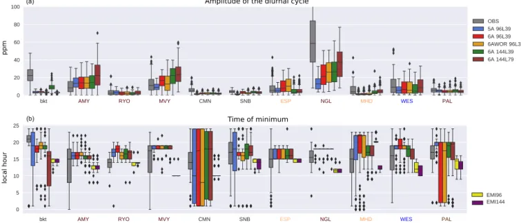
Figure 9a shows the peak-to-peak amplitude of the CO2
mole fractions for eight sites with an amplitude greater than 1.5 ppm for the boreal summer months (JJA). Although sim-ilar conclusions can be drawn in boreal winter, we only de-pict diurnal cycle characteristics for the summer when the diurnal amplitude is the strongest. We can see that for most sites, version 5A underestimates the diurnal amplitude with the exception of AMY, in agreement with previous studies (Geels et al., 2007; Locatelli et al., 2015a). The new physics increases the diurnal amplitude at continental sites AMY, MVY and NGL, especially regarding the extremes. Locatelli et al. (2015a) in their supplement showed that the Mellor and Yamada (1974) scheme strongly increases 222Rn overnight compared to the Louis (1979) scheme used in the 5A
ver-sion. Similar experiments with222Rn lead to the same con-clusion (not shown). The strongest increase of amplitude (up to 10 ppm) is seen with a finer vertical resolution for the con-tinental stations NGL and AMY. A possible explanation is that the CO2 input from the surface is distributed within a
thinner layer. Figure 9b shows box plots of a measure of the phase of the diurnal cycle at the same sites in boreal summer for the CO2-simulated mole fraction and the CO2-prescribed
fluxes. The measure of the phase is defined as the local time at the minimum CO2mole fraction. It typically happens in
the afternoon after the convection has ventilated the PBL and the photosynthesis activity has drained the CO2at the
sur-face. In the GCM, the minimum value of the fluxes to the at-mosphere seems to propagate to the sampling level within a few hours at each site. The new physics affects the amplitude without noticeably ameliorating the timing of the diurnal cy-cle. The timing at mountain site SNB is improved, whereas it is deteriorated at site PAL (516 m). The other sites are not affected by the change of physics. In contrast, the horizontal
Figure 9. (a) Box plots of the peak-to-peak amplitude (maximum concentration minus minimum concentration) of the mean diurnal cycle for July–September for observed (grey) and modelled (colours) CO2for each model simulation during the years 2011–2012. The diurnal
amplitude is calculated from the residual between the raw data and the daily mean. The sites are listed on the abscissa. (b) Box plots of time of minimum crossing for each model. The times for the prescribed CO2are displayed for both horizontal resolutions in yellow (96 × 95) and
purple (144 × 143). Here only the sites with a diurnal amplitude greater than 1 ppm are depicted. The code colour for stations is the same as previously.
resolution seems to have a positive effect both on the timing and the amplitude at coastal site MHD. All versions seem to underestimate the mean amplitude and shift the daytime min-imum earlier at the mountain sites CMN and bkt compared to lower latitude sites. Nonetheless, the amplitude is largely dependent on the sampling location and model level. Mod-els typically show high amplitudes at model levMod-els close to the surface and smaller amplitudes aloft (Law et al., 2008). In order to improve the representation of the diurnal cycle, it might be preferable to choose the level which better fits the observations.
4.3 Validation against independent measurements of vertical profiles of CO2
Errors on CO2 flux estimates by inverse modelling are
thought to be proportional to the vertical mixing efficiency within a column (Stephens et al., 2007; Saito et al., 2013). If a model transports too much tracer from the boundary layer to the free atmosphere, the inverse system will compensate the induced tracer deficit at the surface by modulating the CO2
fluxes. A means of validating the flux estimates is to com-pare the simulated vertical profiles with independent (unas-similated) observations of vertical profiles (Pickett-Heaps et al., 2011). Since only surface measurements have been as-similated, the vertical gradient mainly reflects intrinsic mix-ing efficiency within the column. In this section, we evalu-ate the simulevalu-ated vertical profile against independent aircraft measurements over several regions: Europe, North America,
Brazil, East Asia, greater northern India, northern Southeast Asia at the annual and seasonal scales. The benefit of using the newly developed version is also assessed over these re-gions.
4.3.1 North America and Europe
Over North America, the surface flux pattern has a strong seasonality. In winter, positive fluxes to the atmosphere driven by fossil fuel emissions are mainly located along the east coast whereas in summer, the strongest sink is located over the Midwest states. Because of a large net ecosystem production of organic carbon during the crop plant growth, the Midwest states can contribute to half of the summer uptake in North America (Crevoisier et al., 2010; Sweeney et al., 2015). CO2fluxes over North America are relatively
well constrained by surface observations as seen in Fig. 1. Figure 10 shows the seasonal and annual climatologies of the CO2mole fraction bias (model–observations) on average
over all the North American airborne platforms depicted in Fig. 1. On the whole, the simulated value in the lowest level is overestimated by about 0.5 ppm on an annual basis and by about 1 ppm in winter. This behaviour is seen both for profile sites close to assimilated stations (ESP, LEF, THD, SGP) and for profile sites further away (not shown). The pro-file above 2 km is well simulated except in summer when the bias is about 0.5 ppm. This leads to an overestimated verti-cal gradient between 1 and 3 km in winter. In the inversion system, the overestimated winter gradient would artificially
Figure 10. Bias (model–observations, thick lines) and associated standard deviation (shaded areas) for the monthly CO2vertical profile
differences over North America during the period 2008–2014. The data have first been averaged in 1 km altitude bins per hour and per site, before being averaged among the 12 North American sites of Fig. 1 per month. The statistics are drawn from that ensemble of monthly and spatially averaged values. They are shown for each season (January–March, JFM; April–June, AMJ; July–September, JAS; October– December, OND) and for the whole year. In order to highlight the differences in profile shape, the annual mean of the bias at 3.5 km has been removed for each simulated vertical profile (5A-96L39: −2.0 ppm, 6A-96L39: −2.0 ppm, 6AWOR-96L39: −2.0 ppm, 6A-144L39 and 6A-144L79: 1.3 ppm).
Figure 11. Same as for Fig. 10 but over Europe from the CONTRAIL dataset during the period 2006–2011. The domain is portrayed in Fig. 2.
decrease the estimated fluxes to the atmosphere. The model spread does not exceed 0.5 ppm throughout the year except in summer when it reaches a value of 1.5 ppm at 1.5 km and 1 ppm at ground level. It only explains a small share of the variability (standard deviation) of the differences (about 1– 1.5 ppm). This variability of the differences is comparable among the model versions. The difference between the two physics is responsible for a large portion of the model spread. This can be explained, in part, by the fact that the air mass composition is more influenced by local processes during the summer than at any time of the year. At each site, westerly wind flow prevails throughout the year in the entire free tro-posphere. As the air masses move across the continent, they progressively mix with air coming from the biosphere and from fossil emissions. In summer, the decrease of the wind speed over the middle of the continent and over the east coast results in less homogeneous vertical profiles in the free tropo-sphere (Sweeney et al., 2015). Combined with enhanced con-vection, this effect might emphasize the divergence between
the two physics. The convective inhibition (Fig. 3) as a result of the new physics translates into a lower concentration of 1 ppm at 1.5 km and a higher CO2concentration of 0.6 ppm
in the mid-troposphere as the trapping of negative anomalies of the CO2 mole fraction within the PBL is enhanced. The
CO2 depletion around 1.5 km induced by the new physics
may be due to the vertical transport of negative anomalies by the thermal activity. Combined with the new physics, the land surface scheme also has a strong impact on the summer ver-tical profile as the amount of water vapour and temperature directly influence the vertical mixing through surface buoy-ancy. By inhibiting deep convection, it increases the upper troposphere concentration by 0.5 ppm and decreases the sur-face concentration by 0.5 ppm. The effect of the resolution is modest here.
The figure for Europe (EUR; Fig. 11) shows similar features as for North America, but with smaller model– measurement differences (absolute biases, standard
devia-Figure 12. Same as for Fig. 11 over East Asia (EAS), northern Southeast Asia (NSA) and greater northern India (IND).
tions, model spread), except for the standard deviations in the lower atmosphere that are about 50 % larger.
4.3.2 Indo-Pacific region
Figure 12 presents the profile of the model–observations dif-ference statistics for the CONTRAIL CO2 data over East
Asia, northern Southeast Asia, and greater northern India. They mostly have the same shape: a negative bias close to the surface (up to −8 ppm for greater northern India in OND) and a null one above. The decreasing standard deviations of the differences with height and the small model spread under 1 ppm are similar to EUR, except for greater northern India in the lower atmosphere, where the model spread reaches 2 ppm (up to 4 ppm) at the seasonal scale, in particular at the end of the monsoon season (OND).
In NSA and IND, the negative bias at the annual scale within the boundary layer is likely related to urban sources, close to the airports for these commercial flights. The nega-tive bias was also noticed in NSA and in IND for OND in the study of Lin et al. (2017). We also note that the prescribed surface fluxes have not been well constrained for IND and NSA. For NSA, only station GMI has been assimilated over the period 2006–2011. IND is directly constrained by HLE only, a site that is located in a mountain area at the north-ern edge of the domain: backward trajectories showed that the site HLE samples air masses moving through the Ara-bian desert and northern Africa in winter and those coming from Southeast Asia in summer (Suresh Babu et al., 2011; Lin et al., 2015). The impact of the model set-ups reaches 3 ppm in this region and during AMJ and OND, two inter-mediary seasons. Special care should be taken when assim-ilating new stations in this area. Further to this lack of
mea-0 2 4 6 Rn222 1e 14 0 1 2 3 4 5 6 7 8 9 10 Height (km) WET 0 2 4 6 Rn222 1e 14 DRY
Figure 13. (a) Mean difference between CO2profiles measured and simulated in 2010 at the four Amazonian aircraft sampling sites and an
oceanic CO2background (i.e. 1 CO2) during the dry (left of each panel) and wet (right of each panel) seasons, respectively (solid lines) and
the standard deviation divided by the square root of number of profiles (dashed lines and error bars). The background is estimated from in situ measurements at monitoring stations ASC and RPB, as described in the main text. (b) Same as the top but for the222Rn (ppm). The dry season (red lines) is affected by fires at most sites and is defined here as the period July–October for illustrative purposes only; it does not correspond to all months within the fire season.
surement constraints, the prescribed flux variability in NSA and IND mainly reflects the prior flux variability, while in EAS, fluxes are more robust (Thompson et al., 2016) and the model–observations differences appear comparable to EUR there.
4.3.3 Amazon basin
The CO2surface fluxes over the Amazon basin have not been
directly constrained by observations. The two closest assim-ilated stations are located along the Atlantic coast (Fig. 1). They are representative of the air masses coming off the trop-ical Atlantic Ocean through the troptrop-ical easterly winds (Gatti et al., 2014). Moreover, the assimilation of additional surface and airborne observations has not enabled the variability of the CO2fluxes to be improved so far, at least with this
inver-sion system (Molina et al., 2015). Molina et al. (2015) con-cluded, through several experiments with both global and re-gional models, that this limitation mainly stems from model transport errors and uncertainties on biospheric and fire burn-ing emissions. In this context, we evaluate the sensitivity of the simulated CO2 concentrations to model set-ups at the
four airborne stations featured in Fig. 1: tab, rba, alf, san. The simulated and observed CO2 vertical profiles averaged for
the wet period (January–June) and dry period (July–October) in 2010 are depicted in Fig. 13. All versions poorly represent the shape of the mean observed CO2vertical profiles in the
lower troposphere. The mismatch is particularly amplified
during the dry season. The vertical gradients of the reference 5A-96L39 and of the observations between 1 and 3 km have opposite signs, suggesting issues in the prior fluxes (NEE or/and fire emissions).
The simulated profile is also very sensitive to the subgrid-scale parameterizations for each site, and, to a lesser extent, to the land surface model. At the surface, the difference be-tween the two physics ranges from 2 ppm at san in the dry season to 6 ppm at tab during the wet period. The other set-ups have a modest impact compared to the physics.
The CO2vertical profiles suggest a more mixed lower and
mid-troposphere with the new physics. In order to visualize the behaviour of the two physics, we additionally calculate the corresponding simulated 222Rn profiles with the same sampling strategy, even though we do not have any observa-tions to compare them with. The lower row of Fig. 13 shows that less radon is transported above 5 km in the new physics, suggesting a less dominant role of deep convection. This is confirmed while comparing the simulated mean precipita-tion during the wet and dry period with reference data from NASA’s Global Precipitation Climatology Project (Fig. 14). In the tropics, precipitation is an indicator of the convective activity and we see here that the new physics decreases the mean precipitation (mainly convective) during both periods without showing better agreement with the reference data. The modelling of the precipitation in this region has been shown to be particularly challenging (Lintner et al., 2017).
Figure 14. Observed and simulated mean precipitation (mm day−1) during the wet and dry seasons over each Amazonian sampling site (tab, rba, san, alf). The black dots depict monthly mean precipitations derived from NASA’s Global Precipitation Climatology Project.
The simulated radon profiles suggest that more radon is de-trained above the boundary layers by the thermals in the new physics, especially during the dry season. The strengthening of the thermals when the deep convective scheme is inhibited is a known behaviour of the new physics (Rio and Hourdin, 2008). As a result, the boundary layer of the new physics is more mixed and goes higher.
The lack of realism of the simulated local transport does not impact the CO2fluxes estimated by inverse modelling in
this region, as they have mostly relied on the prior fluxes and long-range transport up to now. However, it limits the poten-tial benefit of assimilating new surface observations there, in line with Molina et al. (2015).
5 Conclusions
We have compared two reference versions of a GCM, LMDz, that have been prepared for, respectively, CMIP5 and CMIP6, from the point of view of the transport of tracers. The more recent version benefits from a more elaborated radiative scheme and subgrid-scale parameterizations, in addition to a refined vertical resolution. The main changes in the physi-cal parameterizations concern boundary layer mixing due to vertical diffusion (Mellor and Yamada, 1974), shallow con-vection (Rio and Hourdin, 2008; Rio et al., 2009), thermo-dynamic effects of ice, cool pools (Grandpeix et al., 2009) and convective triggering and closure assumptions (Rochetin et al., 2013). These main changes have been accompanied over the years by other evolutions of the model physics, by continuous tuning (Hourdin et al., 2017), and by continuous technical changes (including bug introduction and bug fixes) that have diverse impacts. Within this flow of modifications from a large developer group, our evaluation of the two ver-sions is based on a snapshot of the LMDz code in its release 2791, a few months before the start of the CMIP6 simula-tions.
We performed a set of CO2, SF6and222Rn simulations
us-ing those two versions of LMDz at two horizontal resolutions and guided by the ECMWF wind reanalysis for nearly two
decades (1998–2014). In addition, we compared two simu-lations with two different land surface schemes, one using the ORCHIDEE terrestrial surface model and the second us-ing a simplified bulk scheme. In this case, the land surface scheme only controls the heat and latent fluxes at the land– atmosphere interface. The SF6 and 222Rn emissions were
prescribed following the TransCom 3 protocol. The CO2
sur-face fluxes have been optimized beforehand by the assimi-lation of surface observations in a version of LMDz close to the older model version studied here. We have compared the resulting ensemble of simulations with both assimilated and unassimilated CO2observations from a large dataset in
different parts of the globe. This study enabled us to bench-mark the effects of the resolution, land surface scheme and subgrid-scale parameterizations on CO2-simulated values,
which is a fundamental step before implementing the recent developments in our inverse modelling system.
At the surface, the comparison with the assimilated CO2
measurements showed that the land–surface scheme and the vertical resolution have a limited impact compared to the hor-izontal resolution and subgrid-scale parameterizations. The new physics tends to weaken the vertical mixing within the column over continental areas. The annual mean mole fraction values are little modified but the variability at sea-sonal, synoptic and diurnal scales is enhanced at continental and coastal sites. The higher seasonal cycle in the Northern Hemisphere, as a result of a less efficient vertical mixing, af-fects the latitudinal CO2gradient in boreal summer by about
1 ppm, a value that should impact the geographical distri-bution of the CO2surface fluxes estimated by inverse
mod-elling. At the synoptic scale, the higher model variance does not lead to an improved correlation with the measurements: the change of physics increases the amplitude of the synop-tic variability without affecting the phasing. As for the diur-nal cycle, even though the amplitude shows better agreement with the observations, the phasing is not improved by the model set-ups at most CO2monitoring stations, but it heavily
relies on the prior fluxes used in the inversion system. Even though the improved amplitude is promising for assimilating