Development and Analysis of High Order
Neutron Transport–Depletion Coupling
Algorithms
byColin Josey
B.S., University of New Mexico (2013) S.M., Massachusetts Institute of Technology (2015)
Submitted to the Department of Nuclear Science and Engineering in partial fulfillment of the requirements for the degree of Doctor of Philosophy in Nuclear Science and Engineering
at the
MASSACHUSETTS INSTITUTE OF TECHNOLOGY September 2017
c
○ Massachusetts Institute of Technology 2017. All rights reserved. Author . . . .
Department of Nuclear Science and Engineering September 1, 2017 Certified by . . . . Benoit Forget Associate Professor of Nuclear Science and Engineering Thesis Supervisor Certified by . . . . Kord Smith KEPCO Professor of the Practice of Nuclear Science and Engineering Thesis Reader Accepted by . . . .
Ju Li Battelle Energy Alliance Professor of Nuclear Science and Engineering Chairman, Department Committee on Graduate Theses
Development and Analysis of High Order Neutron
Transport–Depletion Coupling Algorithms
by
Colin Josey
Submitted to the Department of Nuclear Science and Engineering on September 1, 2017, in partial fulfillment of the
requirements for the degree of
Doctor of Philosophy in Nuclear Science and Engineering
Abstract
The coupling of depletion and neutron transport together creates a particularly challenging mathematical problem. Due to the stiffness of the ODE, special algorithms needed to be developed to minimize the number of transport simu-lations required. In addition, for stochastic transport, both the time step and the number of particles per time step need to be considered. In recent years, many new coupling algorithms have been developed. However, relatively little analysis of the numeric and stochastic convergence of these techniques has been performed.
In this document, several new algorithms are introduced. Some are improve-ments of current techniques, some are taken from similar problems in other fields, and some are derived from scratch for this specific problem. These were then tested on several test problems to investigate their convergence. With regard to numerical error, the CF4 algorithm (a commutator-free Lie integra-tor) outperformed all tested algorithms. In number of transport simulations to achieve a 0.1% gadolinium relative error, CF4 requires half the simulations. With regard to stochastic error, it was found that once a time step is sufficiently reduced, errors are mostly a function of the number of particles used during the simulation. The remaining variability is due to how stochastic noise propa-gates through each numerical integrator. Using this information, a technique is developed to minimize the cost of running a depletion simulation.
Thesis Supervisor: Benoit Forget
Acknowledgments
I would like to thank all of those who have taught me so much over the course of this project. Specifically, I would like to thank my advisers, Ben Forget and Kord Smith. Without them to bounce ideas off of, many aspects of this project would not exist. In addition, I would like to thank my family for helping me through this project.
This research was funded in part by the Consortium for Advanced Sim-ulation of Light Water Reactors (CASL) under U.S. Department of Energy Contract No. DE-AC05-00OR22725; DOE’s Center for Exascale Simulation of Advanced Reactors (CESAR) under U.S. Department of Energy Contract No. DE-AC02-06CH11357; and by a Department of Energy Nuclear Energy Univer-sity Programs Graduate Fellowship. This research made use of the resources of the High Performance Computing Center at Idaho National Laboratory, which is supported by the Office of Nuclear Energy of the U.S. Department of Energy under Contract No. DE-AC07-05ID14517.
Contents
1 Introduction 17 1.1 Fundamental Equation . . . 18 1.1.1 Computing Coefficients . . . 20 1.1.2 𝐴- and 𝐿-Stability . . . 21 1.1.3 Xenon Instabilities . . . 22 1.2 Implementation Issues . . . 24 1.2.1 Calculating Power . . . 241.2.2 Isomeric Branching Ratios . . . 26
1.2.3 Memory Concerns . . . 26
1.3 Goals . . . 27
2 Current Numerical Methods 29 2.1 Current Depletion Algorithms . . . 29
2.1.1 The Predictor Method . . . 29
2.1.2 Predictor-Corrector . . . 30
2.1.3 Stabilizing 135Xe by Asserting a Solution . . . . 33
2.2 Current Methods from Other Fields . . . 34
2.2.1 Integrators for 𝑦′ = 𝐴(𝑡)𝑦 . . . . 35
2.2.2 Runge–Kutta–Munthe-Kaas Integrators . . . 36
2.2.3 Commutator-Free Methods . . . 39
2.3 Matrix Exponents . . . 40
2.3.1 Chebyshev Rational Approximation . . . 40
2.3.2 Scaling and Squaring . . . 41
2.3.3 Krylov Subspace . . . 42
2.3.4 Exponential Testing . . . 42
3 New Methods 45 3.1 Replacing the Subintegrator in CE/LI and LE/QI . . . 45
3.2 Stochastic Implicit CE/LI and LE/QI . . . 47
3.3 Extended Predictor-Corrector . . . 48
3.4 The Exponential-Linear Method . . . 49
3.5 The Relative Variance of Methods . . . 57
3.6 Adaptive Time Stepping . . . 58
3.6.1 Choice of Error . . . 59
3.6.2 Uncertain Error . . . 62
4 Small-Scale Test Problem 67 4.1 The Facsimile Pin Derivation . . . 68
4.2 The Facsimile Pin Convergence Results . . . 70
4.2.1 First Order Methods . . . 72
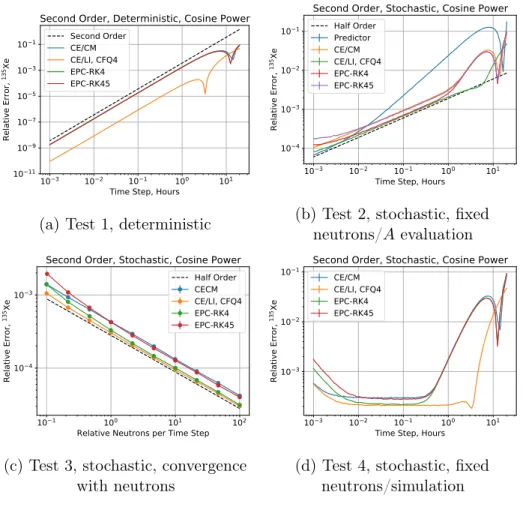
4.2.2 Second Order Methods . . . 75
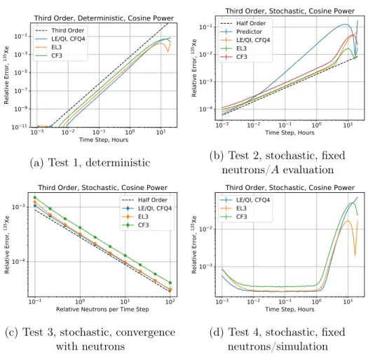
4.2.3 Third Order Methods . . . 77
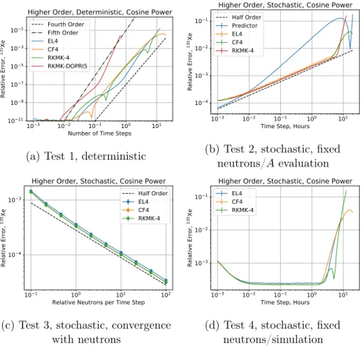
4.2.4 Higher Order Methods . . . 80
4.3 Adaptive Time Stepping on the Facsimile Pin . . . 80
4.3.1 Properties of Distributions During Time Integration . . 80
4.3.2 Hyperparameters of the Multi-Sample Algorithm . . . 85
4.3.3 Comparison of Adaptive Time Stepping Algorithms on the Facsimile Problem . . . 87
4.4 Facsimile Pin Conclusions . . . 89
5 Full Depletion Tests 95 5.1 2D Depletion Test . . . 95
5.1.1 2D Model Reference Solution . . . 97
5.1.2 2D Model Constant Time Step . . . 99
5.1.3 2D Model Adaptive Time Step . . . 105
5.2 3D Depletion Test . . . 112
5.2.1 Reflective Boundary Condition . . . 113
5.2.2 Vacuum Top/Bottom Boundary Conditions . . . 114
5.3 Summary of Full Depletion Tests . . . 114
6 Summary 119 6.1 The Cost of Depletion . . . 120
6.2 Recommendations . . . 123
6.2.1 Recommendations for Deterministic Simulations . . . . 123
6.2.2 Recommendations for Stochastic Simulations . . . 124
6.3 Conclusions . . . 125
A Exponential-Linear Coefficient Tables 127 A.1 EL3 . . . 127
B The Facsimile Pin Equations 131 B.1 Un-Normalized Reaction Rate Reconstruction . . . 131 B.2 Equations . . . 134
List of Figures
1-1 Oscillations in depletion with a short time step . . . 23 1-2 Oscillations in depletion with a long time step . . . 24
2-1 Power as a function of time on the facsimile pin for varying normalization, LE/QI, 4 time steps with one initial CE/CM step of 1 hour . . . 32 2-2 Error between the approximate and reference solution for various
orders of CRAM for time steps from 1 second to109 seconds . 43 2-3 Error between the approximate and reference solution for the
Krylov method with various Arnoldi factorization steps for both inner exponentials . . . 43 2-4 Error between the approximate and reference solution for CRAM
and scaling and squaring from 1 second to 109 seconds . . . . 44
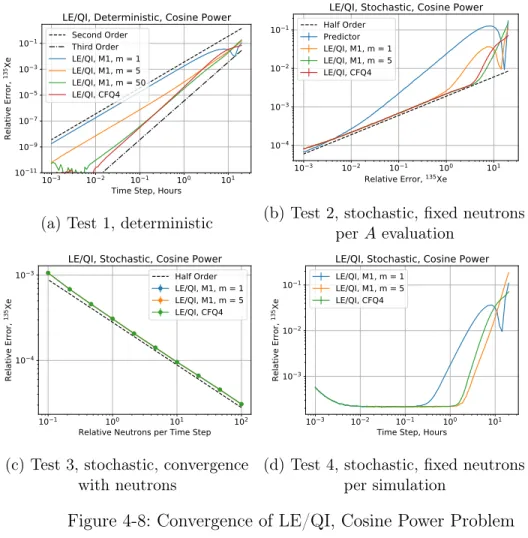
4-1 Decay chain for the facsimile pin problem . . . 68 4-2 The evolution of 135Xe with time in the facsimile pin problem 71 4-3 Convergence of first order methods, cosine power problem . . . 73 4-4 Convergence of first order methods, constant power problem . 74 4-5 Comparison of nuclide and reaction rate relaxation . . . 75 4-6 Convergence of CE/LI, cosine power problem . . . 76 4-7 Convergence of Second Order Methods, Cosine Power Problem 78 4-8 Convergence of LE/QI, Cosine Power Problem . . . 79 4-9 Convergence of third order methods, cosine power problem . . 81 4-10 Convergence of higher order methods, cosine power problem . 82 4-11 Fixed 𝑁 , variable ℎ comparison of error between second and
third order estimates, EL3, constant power . . . 83 4-12 Fixed ℎ, variable 𝑁 comparison of error between second and
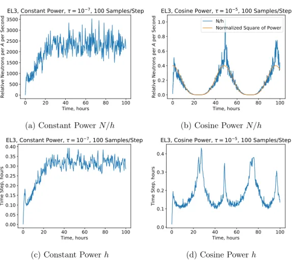
third order estimates, EL3, constant power . . . 84 4-13 The evolution of the optimal 𝑁/ℎ and ℎ for fixed and cosine
power distributions . . . 85 4-14 Contour plots of the log10 figure of merit for a variety of
4-16 Mode 1 ATS scheme results . . . 89 4-17 Mode 2 ATS scheme results . . . 90 4-18 Mode 3 ATS scheme results . . . 91 4-19 Cost as a function of accuracy, facsimile pin, cosine power . . 92 5-1 The 2D depletion geometry . . . 96 5-2 Global error comparison with time, reference comparison . . . 98 5-3 Nuclide error comparison with time, reference comparison . . . 98 5-4 Global error comparison at 𝑡 = 150 days, 4 million neutrons . 101 5-5 Global error comparison at 𝑡 = 150 days, 6-day time step . . . 101 5-6 Nuclide error comparison at 𝑡 = 150 days, 4 million neutrons . 102 5-7 Nuclide error comparison at 𝑡 = 150 days, 6-day time step . . 102 5-8 Global error comparison at 𝑡 = 150 days, 4 million neutrons,
subintegrators . . . 106 5-9 Global error comparison at𝑡 = 150 days, 6-day time step,
subin-tegrators . . . 106 5-10 Nuclide error comparison at 𝑡 = 150 days, 4 million neutrons,
subintegrators . . . 107 5-11 Nuclide error comparison at 𝑡 = 150 days, 6-day time step,
subintegrators . . . 107 5-12 Global error comparison at 𝑡 = 150 days, 4 million neutrons,
stochastic implicit . . . 108 5-13 Nuclide error comparison at 𝑡 = 150 days, 4 million neutrons,
stochastic implicit . . . 108 5-14 Adaptive time stepping results for the nuclide based error
esti-mate . . . 110 5-15 Adaptive time stepping results for the reaction rate based error
estimate . . . 111 5-16 135Xe mean relative error vs. the mean active neutrons per time
step for the reaction rate based error . . . 112 5-17 Mean coefficient of variation of 135Xe for the fully reflected 3D
pin problem, explicit comparison . . . 116 5-18 Mean coefficient of variation of 135Xe for the fully reflected 3D
pin problem, CE/LI and LE/QI subintegrator comparison . . 116 5-19 Mean coefficient of variation of 135Xe for the fully reflected 3D
pin problem, stochastic implicit . . . 116 5-20 Mean coefficient of variation of135Xe for the vacuum top/bottom
3D pin problem, explicit comparison . . . 117 5-21 Mean coefficient of variation of135Xe for the vacuum top/bottom
5-22 Mean coefficient of variation of135Xe for the vacuum top/bottom 3D pin problem, stochastic implicit . . . 117
List of Tables
1.1 Oscillation demonstration simulation parameters . . . 23 1.2 235U MT = 458 data from ENDF-B/VII.1 . . . . 25 1.3 Memory utilization for nuclides and reaction rates for two
dif-ferent reactor models . . . 27
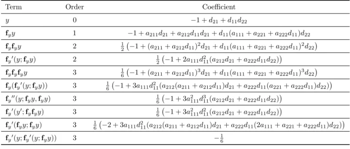
3.1 Formal series coefficients for𝑦− 𝑦approx for a 2-stage exponential linear method to third order . . . 54
4.1 Facsimile Pin Fuel Materials . . . 69 4.2 Facsimile Pin Nuclide Data . . . 69 4.3 Deterministic performance of the first order set, constant power 74 4.4 Statistical performance of the first order set, constant power . 74 4.5 Deterministic performance of CE/LI, cosine power . . . 76 4.6 Statistical performance of CE/LI, cosine power . . . 76 4.7 Deterministic Performance of the Second Order Set, Cosine Power 78 4.8 Statistical Performance of the Second Order Set, Cosine Power 78 4.9 Deterministic Performance of LE/QI, Cosine Power . . . 79 4.10 Statistical Performance of LE/QI, Cosine Power . . . 79 4.11 Deterministic performance of the third order set, cosine power 81 4.12 Statistical performance of the third order set, cosine power . . 81 4.13 Deterministic performance of the higher order set, cosine power 82 4.14 Statistical performance of the higher order set, cosine power . 82 4.15 ATS hyperparameter parametric analysis . . . 86 4.16 ATS Parameter Set . . . 88
5.1 2D fuel pin array reference solution simulation parameters . . 97 5.2 Estimated errors at a time of 150 days for the reference depletion
problem . . . 99 5.3 Estimated maximum time step (days) to achieve accuracy . . 103 5.4 Estimated minimum total active neutrons to achieve 1% accuracy104 5.5 Parameters for the adaptive time stepping simulation . . . 109 5.6 Oscillation simulation parameters . . . 113
6.2 Estimated minimum number of neutrons necessary to achieve
1% accuracy on average in all cells over 150 days . . . 122
6.3 Estimated minimum number of transport solves required to achieve given error for 150 days . . . 122
A.1 Coefficients for the exponential-linear 3rd order method EL3 . 128 A.2 Additional coefficients for the second order component of the non-FSAL version of EL(3,2). All non-listed coefficients are zero. 128 A.3 Additional coefficients for the second order component of the FSAL version of EL(3,2). All non-listed coefficients are zero. . 129
A.4 Coefficients for the exponential-linear 4th order method EL4 . 129 B.1 Polynomial Coefficients (𝐶𝑅,𝑖) for𝜇 . . . 132
B.2 Polynomial Coefficients (𝐶𝜆,𝑖) for𝜆 in Σ . . . 133
B.3 Polynomial Coefficients (𝐶𝑚,𝑖) for Reconstructing𝑄 in Σ . . . 133
B.4 Facsimile Pin Total Atoms, 100 Hours, Reference Solution . . 135
C.1 Geometry for Fuel . . . 137
C.2 Fuel Composition, Full Depletion Problem . . . 138
C.3 Clad Composition, Full Depletion Problem . . . 139
C.4 Gap Composition, Full Depletion Problem . . . 140
Chapter 1
Introduction
Depletion, the transmutation and decay of nuclides within materials under irradiation in a nuclear reactor, is one of the most challenging problems in the field of nuclear engineering. The ODEs that govern the process present a number of challenges. Primarily, the ODEs are extraordinarily stiff. Secondly, the coefficients of the ODE are computed from a neutron transport simulation. The combination of these two issues mean that very special algorithms are required to perform integration efficiently. Further complications arise if the transport is performed via Monte Carlo, as now the solution to the ODEs have a statistical component.
Unfortunately, relatively little analysis on how these special algorithms work has been performed, especially with regard to uncertain coefficients. The result is that many simulations are performed inefficiently. This takes an already computationally intense problem and increases its cost further. The main goal of this document is to reduce the computational cost of depletion, which is done via a thorough analysis of the algorithms. In addition, several new algorithms are proposed for special use cases. An overview of these goals and the entire project is presented in Section 1.3.
This chapter introduces the governing equations of the depletion process, as well as a brief introduction to why these equations are so challenging to solve. In addition, several implementation challenges are briefly introduced, which will be used to guide the design of new algorithms. In Chapter 2, the current state-of-the-art depletion methods, as well as some advanced techniques from other fields, are reviewed. This is followed by Chapter 3, in which several im-provements are introduced as well as some new techniques such as an adaptive time step scheme. Chapter 4 formulates a simple test problem to rapidly test all of these algorithms. From the results of that chapter, a smaller selection of algorithms are then tested on two real depletion problems in Chapter 5. Finally, Chapter 6 summarizes the results, makes algorithm recommendations, and estimates the costs required for full simulations.
1.1
Fundamental Equation
The equation that governs the transmutation and decay of nuclides inside of an irradiated environment is the Bateman equation [48]. Nuclides can be created and destroyed via either decay or transmutation. When these processes are combined, the result is Equation (1.1).
𝑑𝑁𝑖(r, 𝑡) 𝑑𝑡 = ∑︁ 𝑗 [︂∫︁ 𝑑Ω ∫︁ ∞ 0 𝑑𝐸𝜎𝑗→𝑖(r, Ω, 𝐸, 𝑡)𝜑(r, Ω, 𝐸, 𝑡) + 𝜆𝑗→𝑖 ]︂ 𝑁𝑗(r, 𝑡) −∑︁ 𝑗 [︂∫︁ 𝑑Ω ∫︁ ∞ 0 𝑑𝐸𝜎𝑖→𝑗(r, Ω, 𝐸, 𝑡)𝜑(r, Ω, 𝐸, 𝑡) + 𝜆𝑖→𝑗 ]︂ 𝑁𝑖(r, 𝑡) (1.1) Where:
𝑁𝑖(r, 𝑡) = nuclide 𝑖 density at position r and time 𝑡
𝜎𝑖→𝑗(r, Ω, 𝐸, 𝑡) = microscopic cross section of a reaction where nuclide 𝑖
generates nuclide 𝑗 at position r, angle Ω, energy 𝐸 and time 𝑡 𝜑(r, Ω, 𝐸, 𝑡) = neutron flux at position r, angle Ω, energy 𝐸 and time 𝑡
𝜆𝑖→𝑗 = decay constant of nuclide 𝑖 to nuclide 𝑗
As a matter of convenience, the rest of this document assumes that the reactor is discretized into regions in which the cross sections and nuclide densities are constant. This is not strictly necessary; instead one could approximate spatially varying terms with polynomials and integrate the coefficients [18], but the former is the most common approach. This modification yields Equation (1.2), in which an integral over volume has been performed. 𝑁𝑖(𝑐)(𝑡) stands for the atom density of nuclide𝑖 in cell 𝑐.
𝑑𝑁𝑖(𝑐)(𝑡) 𝑑𝑡 = ∑︁ 𝑗 [︂ 1 𝑉𝑐 ∫︁ cell 𝑑r ∫︁ 𝑑Ω ∫︁ ∞ 0 𝑑𝐸𝜎𝑗→𝑖(r, Ω, 𝐸, 𝑡)𝜑(r, Ω, 𝐸, 𝑡) + 𝜆𝑗→𝑖 ]︂ 𝑁𝑗(𝑐)(𝑡) −∑︁ 𝑗 [︂ 1 𝑉𝑐 ∫︁ cell 𝑑r ∫︁ 𝑑Ω ∫︁ ∞ 0 𝑑𝐸𝜎𝑖→𝑗(r, Ω, 𝐸, 𝑡)𝜑(r, Ω, 𝐸, 𝑡) + 𝜆𝑖→𝑗 ]︂ 𝑁𝑖(𝑐)(𝑡) (1.2)
The next consideration is where to get components of the above equation to solve it. The decay constants are the easiest, as they are available from databases such as ENDF/B-VII.1 [14]. The integrals however, require a space-angle-energy neutron transport solution. When a neutron transport solver is given𝑁𝑖 at time 𝑡, a typical reaction rate tally will yield the quantity ^𝑅 given
1.1. FUNDAMENTAL EQUATION in Equation (1.3) [42]. ^ 𝑅(𝑐)𝑖→𝑗(𝑡) = ∫︁ cell 𝑑r ∫︁ 𝑑Ω ∫︁ ∞ 0 𝑑𝐸𝜎𝑖→𝑗(r, Ω, 𝐸, 𝑡)𝑁𝑖(r, 𝑡) ^𝜑(r, Ω, 𝐸, 𝑡) ^ 𝑅(𝑐)𝑖→𝑗(𝑡) = 𝑁𝑖(𝑐)(𝑡) ∫︁ cell 𝑑r ∫︁ 𝑑Ω ∫︁ ∞ 0 𝑑𝐸𝜎𝑖→𝑗(r, Ω, 𝐸, 𝑡) ^𝜑(r, Ω, 𝐸, 𝑡) (1.3)
This is almost but not quite the integral shown in Equation (1.2), the differ-ence being the ^𝜑, which represents the unnormalized flux and not the true flux. To get the ratio between the true flux and the unnormalized flux, power normalization must be performed. The power given an unnormalized flux is given by Equation (1.4). 𝑃other includes energy deposition from scattering and other similar events, as computed using the unit flux. 𝑄(𝑟) and 𝑄(𝑑) are the recoverable quantities of energy emitted given a reaction or decay respectively.
𝑃unit(𝑡) = ∑︁ 𝑖,𝑗 ∫︁ 𝑑r ∫︁ 𝑑Ω ∫︁ ∞ 0 𝑑𝐸𝜎𝑖→𝑗(r, Ω, 𝐸, 𝑡)𝑁𝑖(r, 𝑡) ^𝜑(r, Ω, 𝐸, 𝑡𝑠)𝑄 (𝑟) 𝑖→𝑗(r, Ω, 𝐸) +∑︁ 𝑐,𝑖,𝑗 𝑉𝑐𝑁𝑖(𝑐)(𝑡)𝜆𝑖→𝑗𝑄(𝑑)𝑖→𝑗 + 𝑃other(𝑡) (1.4)
The average of 𝑄(𝑟) is often used to further simplify this calculation, as then the first integral just becomes the sum of ^𝑅𝑖→𝑗(𝑐) 𝑄(𝑟)𝑖→𝑗 for all 𝑐, 𝑖, and 𝑗. A more thorough discussion of power computation is presented in Section 1.2.1. Once 𝑃unit is known, then 𝑅 is given by Equation (1.5).
𝑅𝑖→𝑗(𝑐) (𝑡) = 𝑃 (𝑡) 𝑃unit(𝑡)
^
𝑅(𝑐)𝑖→𝑗(𝑡) (1.5)
This simplifies Equation (1.2) further to the form given in Equation (1.6).
𝑑𝑁𝑖(𝑐)(𝑡) 𝑑𝑡 = ∑︁ 𝑗 [︃ 𝑅(𝑐)𝑗→𝑖(𝑡) 𝑉𝑐𝑁 (𝑐) 𝑗 (𝑡) + 𝜆𝑗→𝑖 ]︃ 𝑁𝑗(𝑐)(𝑡) −∑︁ 𝑗 [︃ 𝑅(𝑐)𝑖→𝑗(𝑡) 𝑉𝑐𝑁𝑖(𝑐)(𝑡) + 𝜆𝑖→𝑗 ]︃ 𝑁𝑖(𝑐)(𝑡) (1.6)
One might note that 𝑁(𝑐)(𝑡) is in both the denominator and numerator in parts of the equation. While it is tempting to cancel it out, one notes by com-parison to Equation (1.3) that𝑁(𝑐)(𝑡) is already cancelled out in the fraction 𝑅(𝑐)(𝑡)/𝑁(𝑐)(𝑡). Care must be taken to ensure that this value is correctly com-puted even when 𝑁𝑖 = 0, by directly computing the integral in (1.3) or by adding near-infinitely dilute quantities of nuclides. This form can be
trans-formed one final time into the form of Equation (1.7). 𝑦′(𝑐)(𝑡) = 𝐴(𝑐)(𝑦, 𝑡)𝑦(𝑐)(𝑡) (1.7) 𝑦(𝑐)𝑖 (𝑡) = 𝑉𝑐𝑁𝑖(𝑐)(𝑡) 𝐴(𝑐)𝑖,𝑗(𝑦, 𝑡) = 𝑅 (𝑐) 𝑖→𝑗(𝑡) 𝑦𝑖(𝑐)(𝑡) + 𝜆𝑖→𝑗 (1.8)
The formation of 𝐴 is then a simple process, given by Algorithm 1.
Algorithm 1 Forming 𝐴 for a cell at time 𝑡 Run Neutronics simulation using densities𝑁 (𝑡)
^
𝑅(𝑐)𝑖→𝑗 ← the tally of reaction 𝑖 → 𝑗
𝑃unit(𝑡)← the power computed from the neutronics simulation 𝑅(𝑐)𝑖→𝑗 ← Equation (1.5)
𝐴(𝑐)𝑖,𝑗(𝑡)← Equation (1.8)
The general form of this equation, Equation (1.9), is a common one in the field of mathematics. As a consequence, there are dozens of methods developed over the years to solve it. The next several chapters detail some of the many techniques available.
𝑦′(𝑡) = 𝐴(𝑦, 𝑡)𝑦(𝑡) (1.9)
A brief introduction into the impact a transport solver has on this ODE is presented in Section 1.1.1. In addition, this particular ODE has a number of sta-bility issues that must be considered during integration. The most fundamental stability issue posed is that of 𝐴 and 𝐿-stability. These are both introduced in Section 1.1.2. The other stability issue is that of xenon oscillations, which is introduced in Section 1.1.3.
1.1.1
Computing Coefficients
There are a wide number of different ways to compute the reaction rates for neutron transport. The broadest categorization of these methods splits the techniques into the stochastic and the deterministic sets. The choice between these two will have a significant impact on depletion and must be considered first.
Deterministic algorithms are the most straightforward. These algorithms solve the neutron transport equation using a fixed process. An example of this kind of method is the Method of Characteristics (MOC) [3]. The result is that for a fixed set of inputs, the output is also fixed. This is convenient, as most
1.1. FUNDAMENTAL EQUATION
numerical analysis techniques rely on this property. Depending on the level of approximation used, deterministic calculations can be performed in a matter of seconds.
Stochastic methods (for example Monte Carlo [11]) are the opposite. These algorithms use random number sequences to compute the solution to the neutron transport equations by following sampled neutrons. The result is that if one takes the exact same geometry with the exact same initial condition but a different random number sequence, the solutions will be different. One of the main issues with Monte Carlo is its convergence rate. The convergence is often proportional to1/√𝑁 , where 𝑁 is the number of particle samples. This convergence rate can make the simulation of a nuclear reactor core with Monte Carlo take several hundreds or thousands of CPU hours to compute.
As such, a deterministic solve can get a fixed, approximate 𝐴 with no stochastic noise in a relatively short amount of time. Stochastic methods can randomly sample𝐴 slowly. These differences will become relevant when choos-ing a depletion algorithm.
1.1.2
𝐴- and 𝐿-Stability
The concepts of𝐴- and 𝐿-stability are important in the design and discussion of depletion algorithms. Both of these stability criterion are based on the solutions to a simplified initial value problem (IVP) of the form shown in Equation (1.10) [9].
𝑦′(𝑡) = 𝜆𝑦(𝑡), 𝑦(0) = 1, 𝜆∈ C, ℜ𝜆 < 0 (1.10) This IVP has an analytic solution of the form 𝑦(𝑡) = 𝑒𝜆𝑡. Now, obviously, if ℜ𝜆 < 0, the analytic solution converges to zero at 𝑡 → ∞. It would thus be valuable if a numerical method also converged to zero on this same problem.
Let us assume one integrates this IVP and generates two successive esti-mates for 𝑦 at time step 𝑛 and 𝑛 + 1, which are separated by a step size of ℎ. A function 𝑅 can be defined as shown in Equation (1.11).
𝑅(𝑧) = 𝑦𝑛+1 𝑦𝑛
(1.11) 𝑧 = 𝜆ℎ
Option one for ensuring a method converges to zero is to ensure that any given choice in time step yields an estimate to 𝑦 closer to zero than the previous estimate. Then, if one took infinite time steps, one is sure to recover the exact answer at 𝑡 =∞. This leads to the 𝐴-stability criterion, which is given by:
Option two additionally states that if one takes a single infinitely large time step, the exact solution should also appear. This leads to the 𝐿-stability criterion:
lim
|𝑧|→∞𝑅(𝑧) = 0,∀𝑧, ℜ𝑧 < 0.
As an example, 𝑅 for explicit Euler and implicit Euler are shown in Equa-tion (1.12) and EquaEqua-tion (1.13) respectively. One can note that explicit Euler will only converge for|1+𝑧| < 1 and that implicit Euler is both 𝐴- and 𝐿-stable.
𝑅explicit(𝑧) = 1 + 𝑧 (1.12)
𝑅implicit(𝑧) = 1
1− 𝑧 (1.13)
One can then extend these criteria for a system of ODEs defined by 𝑦′ = 𝐴𝑦 by eigendecomposing the matrix 𝐴 and redefining 𝑦. The result is that for a system of ODEs, there are many 𝜆s which are given by the eigenvalues of 𝐴, and the requirements must hold for all of them.
So, why is this important for depletion? The problem with depletion is that the span of eigenvalues can be as large as 𝜆 ∈ [−1021, 0]𝑠−1 [39]. If one used the Euler method, then the method will diverge unless:
|1 + 𝜆ℎ| < 1, ∀𝜆.
The result is that the time step ℎ must be on the order of 10−21
seconds or the solution will diverge. This can be mitigated through the use of an 𝐴-stable method. However, there are no solvers that operate purely with linear combinations of function evaluations that are both explicit and 𝐴-stable [37]. This then leads to a choice between implicit methods (which require multiple function evaluations to converge), or nonlinear methods. The added function cost of implicit methods is usually impractical, so all methods presented in Chapter 2 and Chapter 3 use a nonlinear approach. Some methods are also implicit to solve the xenon instability problem.
1.1.3
Xenon Instabilities
The next form of instability is that of xenon instabilities. Xenon oscillations occur when a slight perturbation in the neutron flux increases the power locally in a region of a reactor. This increases the xenon concentration over several hours. As the xenon builds up, the thermal flux goes down, lowering the power. Without feedback of any form, either through thermal, mechanical, or operator-controlled mechanisms, these oscillations can grow. This effect is most prevalent in large geometries.
dis-1.1. FUNDAMENTAL EQUATION
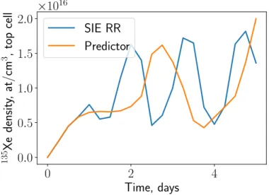
cretized into 8 regions and all boundary conditions are set as reflective. As such, the solution should be uniform. The full model is described in Section 5.2. It is integrated with two different algorithms, the explicit predictor (Section 2.1.1) and the implicit SIE RR (Section 2.1.2.3). SIE is specifically designed to avoid oscillations. As shown, the 135Xe concentration oscillates with a 6-hour time step regardless of algorithm. This process would also likely occur in a real problem if feedback were removed.
0 2 4 Time, days 0.0 0.5 1.0 1.5 2.0 135 Xe densit y, at/cm 3 , top cell ×1016 SIE RR Predictor
Figure 1-1: Oscillations in depletion with a short time step
Predictor SIE RR
Batches Total 5000 5000
Batches Active 2500 2500
Neutrons / Batch 128000 12800 Neutrons Per Time Step 640 million 640 million
Table 1.1: Oscillation demonstration simulation parameters
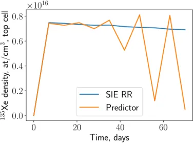
The problem occurs when one wants to take longer steps than the charac-teristic time of the xenon oscillation. When this is done, the oscillation will still attempt to occur as shown in Figure 1-2. With some unstable algorithms, such as predictor, this oscillation will grow until the solution is unusable. With stabilized algorithms, such as SIE RR, this does not.
There is yet no clear mathematical understanding for this particular os-cillation. The few algorithms that solve it do so either by forcing nuclides to take a non-oscillatory solution or by performing an implicit solve. However, the
0 20 40 60 Time, days 0.0 0.2 0.4 0.6 0.8 135 Xe densit y, at/cm 3 , top cell ×1016 SIE RR Predictor
Figure 1-2: Oscillations in depletion with a long time step
particular geometry that generated Figure 1-2 is an extreme case, and many easier geometries can be depleted using normal methods as will be shown in Section 5.1 and Section 5.2.2.
1.2
Implementation Issues
There are three major implementation concerns. The first two, concerning data, do not significantly impact the choice of algorithm, but are mentioned to explain some decisions made in testing later. The two data issues involve the proper computation of power inside of a nuclear reactor (Section 1.2.1) and isomer capture branching ratios (Section 1.2.2). The third issue is that of memory usage. Depletion as a process can take a tremendous amount of memory. Algorithms that require more memory than others can make some geometries impossible to solve with contemporary clusters. The memory issue is briefly discussed in Section 1.2.3.
1.2.1
Calculating Power
The energy released by a single fission is a transient process. There is the prompt energy deposition at the moment of fission and the decay of the daughter nuclei at some time in the future. Ideally, a depletion solver would handle this correctly. The issue is that the total energy deposition is known much more accurately than the prompt energy deposition. For example, the 235U MT = 458 data is given in Table 1.2. Here, the “Total energy less the energy of neutrinos” is
1.2. IMPLEMENTATION ISSUES
known quite accurately, but the sum of the prompt values is not.
Quantity Value (eV) Uncertainty (eV) Kinetic energy of fission products 1.6913× 10⁸ 4.9000× 10⁵
Kinetic energy of prompt fission neutrons 4.8380× 10⁶ 7.0000× 10⁴
Kinetic energy of delayed fission neutrons 7.4000× 10³ 1.1100× 10³
Total energy released by prompt𝛾 6.6000× 10⁶ 5.0000× 10⁵
Total energy released by delayed𝛾 6.3300× 10⁶ 5.0000× 10⁴
Total energy released by delayed𝛽 6.5000× 10⁶ 5.0000× 10⁴
Energy carried away by neutrinos 8.7500× 10⁶ 7.0000× 10⁴
Total energy less the energy of neutrinos 1.9341× 10⁸ 1.5000× 10⁵ Table 1.2: 235U MT = 458 data from ENDF-B/VII.1
This presents a choice on where one wants to approximate, and as such there are a number of options. The first is to simply assume a prompt energy deposition for all recoverable fission energy. Then, to compute the energy from neutron capture one can either track the fission products and capture products separately or compute a time integral approximation for total energy released per capture. The first option requires a more complicated solver and runs into memory issues (see Section 1.2.3). The second option is the one used in CASMO-5 [41], and has the issue that the capture energy deposition is spectrum-dependent.
A second option is to consider prompt and delayed energy separately. This restores temporal accuracy. However, since the total less neutrinos fission value is known quite accurately but the prompt value is not, the uncertainty will be higher. A possible improvement is to compute the total recoverable energy released from the decay of the fission yield spectrum via the decay chain and subtract it from the total less neutrino value to get an effective “prompt” value. Thus, the high accuracy total less neutrino MT = 458 value is conserved and one still gets transient energy deposition.
A third option is to fold an approximate neutron capture value into the prompt fission (for example, by computing approximate energy per capture and captures per fission). The result, usually around 200 MeV for 235U , is extremely easy to implement, but is both spectrum-dependent and temporally inaccurate.
The final option is to take the third option and track decay heat using a decay heat correlation ODE. This technique, presented in [40], restores temporal information to method three. However, these correlations are also spectrum-dependent.
For this document, option three with 200 MeV for all fissionable isotopes will be used unless otherwise noted, as it is simple, easy to implement, and
has little to no bearing on the comparison of the numerical methods. It is recommended to not use this technique in a real depletion solver.
1.2.2
Isomeric Branching Ratios
For certain reactions, the most well-known being 241Am (n,𝛾), several results can occur. For this example, either 242Am or 242mAm can be produced. In general, two approaches have been taken for the computation of the rate of production of each isomer. Option one is to use pre-computed branching ratios in which the branching ratio has been integrated over an approximate energy spectrum of the neutron flux. Option two is to recompute the branching ratio using the actual flux for each function evaluation. The second method typically yields results closer to experiment, but it is still very sensitive to the quality of the underlying library [21].
For the depletion solver used in this paper, constant branching ratios from the Serpent wiki [1] will be used. While these are less accurate than proper energy dependent branching ratios, current versions of OpenMC do not support directly tallying production of isomers.
1.2.3
Memory Concerns
The last major implementation concern is the minimization of memory utiliza-tion. In the ENDF-B/VII.1 library, there are roughly 3800 nuclides with 2000 reaction channels in the set of fission, (n, 𝛾), (n,p), (n,𝛼), and (n, xn). There are a number of ways to simplify this decay chain [20], but this analysis will be performed using these full decay chains.
There are several ways to tally reaction rates. Option one is to simply directly tally each channel, for a total of approximately 2000 values. Option two is to use a coarse group flux, such as 63 groups, and use spectrum-dependent group collapsed cross sections to compute reaction rates [23]. While efficient, this limits the ability to analyze reactors with spectra significantly different from that used to generate the cross section library. Option three is to tally an ultrafine group flux, which can require up to 43000 values [22]. Depending on implementation, the flux-based tallies are much faster than reaction rate tallies. For this research, the first option will be used.
Two reactor models will be discussed. Both of them are based on the specifications of the Seabrook Station reactor listed in Appendix K of [47]. This reactor has 50952 fuel pins, each with an active height of 365.8 cm. The “medium accuracy” model discretizes each pin into 24 axial regions, each with a height of 15.2 cm. The “high accuracy” model discretizes the axial dimension into 366 regions. In addition, each pin is radially discretized into 10 equal volume rings. As such, the medium accuracy model has 1.22 million regions,
1.3. GOALS
Model (GB) Medium High Nuclides 37.2 5700 Reaction Rate Tally 19.6 3000 Coarse Flux 0.6 93 Fine Flux 420.6 64200
Table 1.3: Memory utilization for nuclides and reaction rates for two different reactor models
and the high accuracy model has 186 million regions.
Assuming double precision to store reaction rates and nuclides, each region will require 30.4 kB to store nuclides and 16 kB to store reaction rates. The resulting memory usage for both reactor examples is listed in Table 1.3. Regard-less of what one chooses for the high accuracy model, the memory utilization will be well in excess of contemporary single node computer memory limits. As such, domain decomposition would be essential. Similarly, the fine flux tally may make even the medium model impractically expensive.
Bringing this back to the choice of algorithm, some high order methods require the storage of multiple reaction rates or nuclide quantities. This increase in cost, coupled with the fact that the memory requirements are already very large may make some problems impractical to solve. This increase in memory utilization must be balanced against accuracy and stability requirements.
1.3
Goals
The primary goal of this project is to accelerate depletion simulations to enable full core reactor simulations. However, this is a fairly broad statement, so it is worthwhile to consider how one could go about this. Every algorithm has a number of properties: arithmetic cost, accuracy, stability, and memory requirements. Each of these can be a viable avenue to improve depletion.
The arithmetic cost of an algorithm is the number of raw mathematical operations necessary to complete a time step. For many algorithms, this cost is dominated by the number of matrix exponentials used. For some algorithms, specifically the polynomial algorithms CE/LI (see Section 2.1.2.1) and LE/QI (see Section 2.1.2.2) it is possible to reduce the number of matrix exponentials without compromising accuracy by performing the integration in a different way. This improved algorithm is introduced in Section 3.1.
The accuracy of an algorithm is arguably its most important property, and any improvements would be welcome. Current depletion methods mostly all come from the same family of algorithms, the predictor-corrector family, which
are discussed in Section 2.1.2. Several other families of algorithms were investi-gated. One such family, the commutator-free Lie integrators (see Section 2.2.3), were developed in other fields to solve mathematically similar problems. In addition, two new families of algorithms (extended predictor-corrector, Sec-tion 3.3, and exponential-linear, SecSec-tion 3.4) were derived from scratch in the search for improved accuracy.
As mentioned in Section 2.1.3, the stability of methods is also very important to a depletion algorithm. One tested improvement was to recast the CE/LI and LE/QI methods into an implicit form, which was done in Section 3.2.
Finally, with regard to memory, the memory requirements for all new al-gorithms were computed and compared against current methods. The result is a balancing act between the capability of an algorithm and the memory requirements of said algorithm. This balancing act is sensitive to a user’s needs.
Chapter 2
Current Numerical Methods
In this chapter, current methods for the solution of 𝑦′ = 𝐴(𝑦, 𝑡)𝑦 will be discussed. These are all𝐿-stable methods. Except for stochastic implicit Euler, all methods are also explicit. Section 2.1 presents an overview of the algorithms that are currently used in depletion. This includes the predictor and predictor-corrector families. Section 2.2 then presents some of the techniques commonly used in other fields such as the Runge–Kutta–Munthe-Kaas methods and other Lie algebra based integrators. Finally, since all of these algorithms make heavy use of the matrix exponential, important considerations for matrix exponential algorithms are shown in Section 2.3.
2.1
Current Depletion Algorithms
The majority of current depletion methods reside in the matrix exponential predictor and predictor-corrector families of algorithms. These methods make various approximations to 𝐴 and then leverage the matrix exponential (dis-cussed more thoroughly in Section 2.3) to integrate forwards in an 𝐿-stable manner. While these algorithms are easy to implement and easy to understand, they are more limited in construction when compared to other methods.
2.1.1
The Predictor Method
The easiest way to make an 𝐿-stable method for depletion is to approximate 𝐴 as the constant matrix 𝐴𝑛 over an interval 𝑡 ∈ [𝑡𝑛, 𝑡𝑛+ ℎ]. Under these circumstances, the ODE now has, in principle, an analytic solution, given in Equation (2.1).
𝐴𝑛 = 𝐴(𝑦𝑛, 𝑡𝑛)
The function “expm” is the matrix exponential. This method, while extremely simple, is not without drawbacks. Structurally, the algorithm error converges 𝒪(ℎ). As such, asymptotically, the error is proportional to the step size. Changes in 𝐴 during a time step are completely ignored, resulting in errors resolving rapid changes in reaction rates (for example, irradiation of a burnable poison). As such, predictor is often too inefficient to use.
2.1.2
Predictor-Corrector
The predictor-corrector family is a set of multi-stage improvements over the predictor method. Using values of 𝑦 already known, several values of 𝐴 are computed. Then,𝑦 is integrated using these values to some point in the future (the prediction stage). 𝐴 is evaluated at this predicted 𝑦, and the new value of 𝐴 is then used to re-integrate to 𝑦𝑛+1 (the correction stage). Many such methods are available. Several are listed in [30].
The simplest example would be the CE/CM algorithm used in MCNP6 [19]. The algorithm follows Equation (2.2).
𝑦𝑛+1/2= expm (︂ ℎ 2𝐴(𝑦𝑛, 𝑡𝑛) )︂ 𝑦𝑛 𝑦𝑛+1= expm(︀ℎ𝐴(𝑦𝑛+1/2, 𝑡𝑛+1/2))︀ 𝑦𝑛 (2.2) Here, the value of 𝑦 at the midpoint is estimated using 𝐴 at the beginning of time. Then, 𝐴 is evaluated using this midpoint estimate and integrated to the end of time. This algorithm has a number of advantages, the main one being that the solution converges𝒪(ℎ2). However, it is not the only option available. 2.1.2.1 CE/LI
The CE/LI algorithm, used by default in Serpent [34], takes a slightly different approach. In this algorithm, the initial guess of 𝐴 is integrated to the end of the interval, and an approximate𝐴 that is strictly dependent on time is formed by linear interpolation. The process is shown in Equation (2.3).
𝑦𝑛+1(𝑝) = expm (ℎ𝐴(𝑦𝑛, 𝑡𝑛)) 𝑦𝑛 𝐴𝑙(𝑡) = 𝐴(𝑦𝑛, 𝑡𝑛) (︂ 1− 𝑡− 𝑡𝑛 ℎ )︂ + 𝐴(𝑦𝑛+1(𝑝) , 𝑡𝑛+1) 𝑡− 𝑡𝑛 ℎ ^ 𝑦′(𝑡) = 𝐴𝑙(𝑡)^𝑦(𝑡), 𝑦(𝑡^ 𝑛) = 𝑦𝑛 𝑦𝑛+1 = ^𝑦(𝑡𝑛+ ℎ) (2.3)
There are a number of ways to solve the final, simplified ODE. The CMCDT code uses the VODE algorithm to integrate it directly [10]. Serpent uses a
2.1. CURRENT DEPLETION ALGORITHMS
matrix exponential substepping algorithm. For each substep,𝑠, 𝐴𝑙is integrated. Then, the end result is computed via Equation (2.4). 𝑚 = 5 is often used.
𝐴𝑠=
∫︁ 𝑡𝑛+𝑚𝑠ℎ
𝑡𝑛+𝑠−1𝑚 ℎ
𝐴(𝑠)𝑑𝑠
𝑦(𝑡𝑛+ ℎ) = expm (𝐴𝑚) expm (𝐴𝑚−1) . . . expm (𝐴1) 𝑦(𝑡𝑛) (2.4)
In Section 2.2.1, this will be demonstrated to be a very simple multistep Magnus integrator [5]. There are many other choices of Magnus integrators, and some will be tested as replacements in later chapters. However, whatever choice one makes with the secondary integrator, the overall order of the method will be shown to be limited to 𝒪(ℎ2).
2.1.2.2 LE/QI
Extending the CE/LI idea from the previous method, one could contemplate forming polynomials using information from previous time steps. This is the approach used in the LE/QI method [27], in which a linear polynomial is used to predict, and a quadratic one to correct. The predictor stage is shown in Equation (2.5) and the corrector stage is shown in Equation (2.6). Here, 𝐴last and 𝐴0 are the value of 𝐴 at 𝑡𝑛− ℎ1 and 𝑡𝑛, respectively, and integration is performed to 𝑡𝑛+ ℎ2. 𝐴𝑙(𝑡) =− 𝑡− 𝑡𝑛 ℎ1 𝐴last+ (︂ 1 + 𝑡− 𝑡𝑛 ℎ1 )︂ 𝐴0 ^ 𝑦𝑙′(𝑡) = 𝐴𝑙(𝑡)^𝑦𝑙(𝑡), 𝑦𝑙(𝑡𝑛) = 𝑦𝑛 𝑦𝑙 = ^𝑦𝑙(𝑡𝑛+ ℎ2) (2.5) 𝐴1 = 𝐴(𝑦𝑙, 𝑡𝑛+ ℎ2) 𝐴𝑞(𝑡) = (︂ − ℎ2(𝑡− 𝑡𝑛) ℎ1(ℎ1+ ℎ2) + (𝑡− 𝑡𝑛) 2 ℎ1(ℎ1+ ℎ2) )︂ 𝐴last + (︂ 1− (ℎ1 − ℎ2)(𝑡− 𝑡𝑛) ℎ1ℎ2 − (𝑡− 𝑡𝑛)2 ℎ1ℎ2 )︂ 𝐴0 + (︂ ℎ1(𝑡− 𝑡𝑛) ℎ2(ℎ1+ ℎ2) + (𝑡− 𝑡𝑛) 2 ℎ2(ℎ1+ ℎ2) )︂ 𝐴1 ^ 𝑦𝑞(𝑡) = 𝐴𝑞(𝑡)^𝑦𝑞(𝑡), 𝑦𝑞(𝑡𝑛) = 𝑦𝑛 𝑦𝑛+1= ^𝑦𝑞(𝑡𝑛+ ℎ2) (2.6)
0
20
40
60
80
100
Time, hours
165.65
165.70
165.75
165.80
165.85
165.90
165.95
166.00
Power, W
Facsimile Pin, Constant Power
Correct
Unnormalized
Normalized at Start, 5 substeps
Integral Normalized, 5 substeps
Figure 2-1: Power as a function of time on the facsimile pin for varying nor-malization, LE/QI, 4 time steps with one initial CE/CM step of 1 hour
The asymptotic order of the method can be sensitive to the integrator used to perform the simplified ODEs. In Section 4.2.3, the convergence with several integrators will be analyzed.
For both of the polynomial-based algorithms, it is additionally possible to slightly tweak how integration is performed to improve accuracy [28]. The idea is that while the power is normalized for each function evaluation, the power is not in fact constant over the time step. Additionally, the integral energy deposition over the time step is usually not correct. This discrepancy is shown in Figure 2-1, in which the LE/QI method is used to integrate the facsimile pin problem from Chapter 4. The unnormalized power is off by a maximum of 0.2%. One avenue of improvement is to renormalize the power at each substep using either the beginning of time or midpoint power. Another avenue is to add the following ODE to the matrix exponential:
𝑑𝑞 𝑑𝑡 = ∑︁ 𝑖,𝑗 𝑄(𝑟)𝑖→𝑗Σ𝑖→𝑗𝑦𝑖(𝑡) + ∑︁ 𝑖,𝑗 𝑄(𝑑)𝑖→𝑗𝜆𝑖→𝑗𝑦𝑖(𝑡), 𝑞(𝑡0) = 0
where𝑞 is the energy deposited during a substep. By renormalizing the reaction rates with the result for this ODE, one can achieve more accurate results. The beginning of substep and integral renormalization results are also shown in Figure 2-1, in which both improve results greatly.
The main drawback to these improvements is that the renormalization makes numerical analysis far more difficult. As such, it is difficult to make any guarantees about the performance of these algorithms after renormalization.
2.1. CURRENT DEPLETION ALGORITHMS
Secondarily, the integral method requires multiple matrix exponentials during iteration and the substep renormalization requires substeps. This added cost may make these algorithms impractical for simpler deterministic simulations.
2.1.2.3 Stochastic Implicit Methods
The stochastic implicit Euler (SIE) method was developed in order to solve the xenon oscillation problem [15, 16]. The predictor method is transformed into the implicit form and stochastic gradient descent is used to solve for the nuclide quantity and reaction rate that forms a consistent system. This results in an algorithm that takes the form of Equation (2.7). This specific form is the “relaxation of the neutron flux” version, which, since the computation of reaction rates from the flux is a linear operation, can be recast as a “relaxation of the reaction rate”. An alternative form is to compute the mean of the nuclides instead. 𝑦𝑛+1(0) = expm(ℎ𝐴(𝑦𝑛, 𝑡𝑛))𝑦𝑛 𝐴(𝑖)𝑛+1 = 𝐴(𝑦𝑛+1(𝑖) , 𝑡𝑛+1) ¯ 𝐴(𝑖)𝑛+1 = 1 𝑖 + 1 𝑖 ∑︁ 𝑗=0 𝐴(𝑗)𝑛+1 𝑦𝑛+1(𝑖) = expm(ℎ ¯𝐴(𝑖−1)𝑛+1 )𝑦𝑛 𝑦𝑛+1 = 𝑦𝑛+1(𝑚) (2.7)
Here,𝑚 is the number of substeps, and 𝑖 is the current substep. In the original paper, a value of 𝑚 = 10 was used.
Typically, the flux will tend to counter a xenon oscillation, which will even-tually bring it back to equilibrium. For every substep, the flux is allowed to counter the current xenon oscillation. The averaged reaction rate will then result in a smaller xenon oscillation for the next substep. For a sufficiently large 𝑚, the numerical oscillations will dampen out completely.
While this method can help substantially with xenon oscillations, it is also asymptotically first order. So, while the method is very stable, it is not very accurate. This limits its practical use.
2.1.3
Stabilizing
135Xe by Asserting a Solution
Another way to eliminate xenon oscillations is to simply assert that the solution takes a particular form. There are two methods derived for Monte Carlo to improve 135Xe stability. The first, tested in [29], is to assume that both 135Xe and 135I are in equilibrium. To enforce this, reaction rates are tallied for every batch of a Monte Carlo simulation. Then, using these values, the equilibrium
135Xe and 135I values are solved for and used in the next batch. Depletion is performed normally, but the final 135Xe and 135I values are overwritten by the mean during the active cycles of the simulation. This method acts similar to SIE in allowing the flux to counter the oscillation, but it also eliminates any time evolution of either nuclide from the problem.
The second method, presented in [50] operates much the same, except it is no longer assumed that 135Xe and 135I are in equilibrium. The assumption is instead that the initial concentrations are zero at𝑡 = 0. Each batch is updated by computing the solution to Equation (2.8) with this initial condition. In effect, these two nuclides are handled by a single step of stochastic implicit Euler, while all other nuclides are handled normally.
𝑁𝐼′(𝑡) =∑︁𝛾𝐼Σ𝑓𝜑− 𝜆𝐼𝑁𝐼(𝑡)
𝑁𝑋𝑒′ (𝑡) =∑︁𝛾𝑋𝑒Σ𝑓𝜑 + 𝜆𝐼𝑁𝐼(𝑡)− (𝜎𝑎𝑋𝑒𝜑 + 𝜆𝑋𝑒)𝑁𝑋𝑒(𝑡) (2.8) The result is that the nuclide concentration of 135Xe and 135I can evolve in time using a single step of a first order algorithm. For small 𝑡, the xenon concentration can vary. As 𝑡 increases, the result approaches the equilibrium solution above.
Both algorithms have been shown to successfully stabilize the depletion process. However, since the iodine and xenon concentrations are updated within the transport operator, these approaches are incompatible with a depletion wrapper approach. In addition, overwriting the concentrations at the end of the depletion has an unknown impact on the numerical properties of both algorithms.
2.2
Current Methods from Other Fields
In order to truly improve the state-of-the-art in depletion, it is worthwhile to consider algorithms from other fields. This is the primary motivation behind deriving depletion in the form 𝑦′ = 𝐴(𝑦, 𝑡)𝑦. Integration of stiff equations of this form are a relatively popular topic in the numerical method field, so a huge number of options are available.
First, a brief detour in Section 2.2.1 is made to discuss solutions for the nonautonomous linear ODE𝑦′ = 𝐴(𝑡)𝑦. Then, the Runge–Kutta–Munthe-Kaas family are introduced in Section 2.2.2, followed by the commutator-free Lie integrator family in Section 2.2.3.
2.2. CURRENT METHODS FROM OTHER FIELDS
2.2.1
Integrators for
𝑦
′= 𝐴(𝑡)𝑦
In the earlier predictor-corrector discussion, it was noted that the nonau-tonomous linear ODE appears a number of times as a subproblem that needs to be solved. The Magnus expansion is an infinite series solution to this ODE [5]. The Magnus expansion takes the form of Equation (2.9).
𝑦(𝑡) = exp Ω(𝑡)𝑦(0) Ω(0) = O Ω(𝑡) = ∞ ∑︁ 𝑘=1 Ω𝑘(𝑡) (2.9)
Essentially, the solution to 𝑦(𝑡) is given by a single matrix exponential of the matrix Ω(𝑡). This matrix is formed via an infinite sum of terms, of which the first three are given below. Here, [·, ·] is the matrix commutator, where [𝐴, 𝐵] = 𝐴𝐵− 𝐵𝐴. Ω1(𝑡) = ∫︁ 𝑡 0 𝐴(𝑡1) 𝑑𝑡1 Ω2(𝑡) = 1 2 ∫︁ 𝑡 0 ∫︁ 𝑡1 0 [𝐴(𝑡1), 𝐴(𝑡2)] 𝑑𝑡2𝑑𝑡1 Ω3(𝑡) = 1 6 ∫︁ 𝑡 0 ∫︁ 𝑡1 0 ∫︁ 𝑡2 0 ([𝐴(𝑡1), [𝐴(𝑡2), 𝐴(𝑡3)]] + [𝐴(𝑡3), [𝐴(𝑡2), 𝐴(𝑡1)]]) 𝑑𝑡3𝑑𝑡2𝑑𝑡1
Further terms become increasingly complex. One way to transform this into an effective integrator is to truncate the sum in Equation (2.9). If accuracy is still too low, one could perform substepping in which, instead of integrating in one shot to 𝑡 + ℎ, 𝑚 integrations of ℎ/𝑚 are performed. If one performs this substepping with Ω truncated to Ω1, the result is Equation (2.10). This happens to be identical to the substepping method used for the CE/LI and LE/QI predictor-corrector methods.
𝐴𝑠 =
∫︁ 𝑡𝑛+𝑚𝑠ℎ
𝑡𝑛+𝑠−1𝑚 ℎ
𝐴(𝑠)𝑑𝑠
𝑦(𝑡𝑛+ ℎ) = expm (𝐴𝑚) expm (𝐴𝑚−1) . . . expm (𝐴1) 𝑦(𝑡𝑛) (2.10)
A much cheaper approach than directly evaluating the expansion is to form a quadrature. There are a wide variety of quadrature options. One option, Equation (2.11), only requires one matrix exponential, but requires matrix
commutators in order to do so [5]. 𝑐 = 1 2 ∓ √ 3 6 𝐴𝑖 = 𝐴(𝑡 + 𝑐𝑖ℎ) Ω[4](ℎ) = ℎ 2(𝐴1+ 𝐴2)− ℎ2√3 12 [𝐴1, 𝐴2] 𝑦(𝑡 + ℎ) = exp(︀Ω[4](ℎ))︀ 𝑦(𝑡) (2.11)
Unfortunately, this particular method proved to be unstable during testing. An alternative form, and one that did not have such an issue, is the commutator-free integrator shown in Equation (2.12) [46]. This form removes the need to compute commutators in exchange for requiring multiple matrix exponentials. This algorithm will be abbreviated as “CFQ4” in the rest of the paper.
𝑐 = 1 2 ∓ √ 3 6 𝑎 = 1 4 ± √ 3 6 𝐴𝑖 = ℎ𝐴(𝑡 + 𝑐𝑖ℎ) 𝑦(𝑡 + ℎ) = exp (𝑎2𝐴1+ 𝑎1𝐴2) exp (𝑎1𝐴1+ 𝑎2𝐴2) 𝑦(𝑡) (2.12)
It is unclear why one works and the other does not, but there are at least a few cases where the use of commutators reduces the stability of numerical integration [45]. Additionally, methods based on the Magnus expansion directly may fail if the expansion does not converge. This can happen if
∫︁ 𝑡
0 ‖𝐴(𝑠)‖
2𝑑𝑠 ≥ 𝜋.
The other problem is that the eigenvalues of Ω are not known very rigorously. This can cause issues with the Chebyshev rational approximation matrix ex-ponential recommended for use with depletion (see Section 2.3).
2.2.2
Runge–Kutta–Munthe-Kaas Integrators
The Runge–Kutta–Munthe-Kaas (RK-MK) integrators are a relatively recent innovation in the field of numerical integrators. By leveraging different expo-nential maps, RK-MK acts as a coordinate-free form of Runge-Kutta [26]. This flexibility allows one to solve a problem using an exponential map of their choice. As such, “exp” will be used instead of “expm,” as this is a more general
2.2. CURRENT METHODS FROM OTHER FIELDS
solution. In the depletion case, the exponential map of interest is the matrix exponential. The method is as follows. Given Equation (1.9), the solution is asserted to be
𝑦(𝑡) = exp(Θ(𝑡))𝑦0.
One can then derive a new ODE to solve for the matrix Θ, which is given by Equation (2.13). Θ′(𝑡) = dexp−1Θ(𝑡)(𝐴(𝑦, 𝑡)), Θ(0) = O (2.13) dexp−1𝐴 (𝐶) = ∞ ∑︁ 𝑗=0 𝐵𝑗 𝑗! ad 𝑗 𝐴(𝐶) ad0𝐴(𝐶) = 𝐶 ad𝑗𝐴(𝐶) =[︀𝐴, ad𝑗−1 𝐴 (𝐶) ]︀
Here,𝐵𝑗 are the Bernoulli numbers, ad𝐴 is the adjoint action, and[·, ·] is the Jacobi-Lie bracket (in the matrix exponential case, this is also the matrix commutator). Equation (2.13) can then be solved with Runge-Kutta.
Given an explicit Butcher’s tableau [9] of the form shown in Equation (2.14), the resulting algorithm takes the form of Algorithm 2. Here, dexp−1(Θ𝑘, 𝐴𝑘, 𝑝) is the 𝑝− 1 order truncation of dexp−1
Θ𝑘(𝐴𝑘).
Algorithm 2 Runge–Kutta–Munthe-Kaas Explicit Form 𝑝← the order of the underlying Runge–Kutta scheme 𝑣 ← the number of stages
𝑖← 0
𝑦𝑛 ← the current value of 𝑦 for 𝑖≤ 𝑠 do Θ𝑖 ← ∑︀𝑖−1 𝑗=1𝑎𝑖,𝑗𝐹𝑗 𝐴𝑖 ← ℎ𝐴(exp(Θ𝑖)𝑦𝑛, 𝑡𝑛+ 𝑐𝑖ℎ) 𝐹𝑖 ← dexp−1(Θ𝑖, 𝐴𝑖, 𝑝) 𝑖← 𝑖 + 1 end for Θ←∑︀𝑣 𝑗=1𝑏𝑗𝐹𝑗 𝑦𝑛+1 ← exp(Θ)𝑦𝑛
𝑐1 𝑐2 𝑎21 𝑐3 𝑎31 𝑎32 .. . ... ... . .. 𝑐𝑠 𝑎𝑠1 . . . 𝑎𝑠,𝑠−1 𝑏1 . . . 𝑏𝑠,𝑠−1 𝑏𝑠 . (2.14)
One might notice some level of similarity to prior methods. Applying Al-gorithm 2 to that of the Butcher’s tableau in Equation (2.15) (which is the explicit Euler tableau) results in the method in Equation (2.16). This exactly matches that of predictor.
0 1 (2.15) Θ1 = O 𝐴1 = ℎ𝐴(𝑡𝑛, 𝑦𝑛) 𝐹1 = dexp−1(Θ1, 𝐴1, 1) = 𝐴1 Θ = 𝐹1 𝑦𝑛+1= exp(Θ)𝑦𝑛= exp (ℎ𝐴(𝑡𝑛, 𝑦𝑛)) 𝑦𝑛 (2.16)
Similarly, let us consider the tableau given by Equation (2.17). The resulting method is Equation (2.18). Aside from the commutator in 𝐹2, it is otherwise identical to the CE/CM predictor-corrector method.
0 1 2 1 2 0 1 . (2.17)
2.2. CURRENT METHODS FROM OTHER FIELDS Θ1 = O 𝐴1 = ℎ𝐴(𝑡𝑛, 𝑦𝑛) 𝐹1 = dexp−1(Θ1, 𝐴1, 2) = 𝐴1 Θ2 = 𝐹1 2 𝐴2 = ℎ𝐴 (︂ 𝑡𝑛+ ℎ 2, exp(Θ2)𝑦𝑛 )︂ 𝐹2 = dexp−1(Θ2, 𝐴2, 2) = 𝐴2− 1 2[Θ2, 𝐴2] Θ = 𝐹2 𝑦𝑛+1 = exp(Θ)𝑦𝑛 (2.18)
However, it does get a bit more interesting. The use of dexp−1(Θ𝑖, 𝐴𝑖, 𝑝) is enough to guarantee order 𝑝, but it is not the minimum-cost case. 𝐹 can be reduced further using Lie-Butcher series [36]. As it turns out, the commutator is not required for second order methods. It is only order three and higher in which commutators are required.
There are a few issues with RK-MK schemes when applied to depletion. At least a few are shared with the Magnus integrators in the previous section: commutators may reduce the stability of the method and the eigenvalues of Θ are not known rigorously. Additionally, as the order increases, the number of commutators increases, which takes time to compute and consumes more memory.
2.2.3
Commutator-Free Methods
The commutator-free methods attempt to alleviate a few of the issues with RK-MK methods. By using multiple exponentials per function evaluation, it becomes possible to create a high order method without the use of commutators [13]. Similar to RK-MK, any exponential map can be used with this algorithm, but for depletion a matrix exponential will be used. The algorithm takes the form of Equation (2.19). 𝑌𝑟 = exp (︃ ∑︁ 𝑘 𝛼𝑘𝑟𝐽𝐹𝑘 )︃ . . . exp (︃ ∑︁ 𝑘 𝛼𝑘𝑟1𝐹𝑘 )︃ 𝑦0 𝐹𝑟 = ℎ𝐴(𝑌𝑟) 𝑦1 = exp (︃ ∑︁ 𝑘 𝛽𝐽𝑘𝐹𝑘 )︃ . . . exp (︃ ∑︁ 𝑘 𝛽1𝑘𝐹𝑘 )︃ 𝑦0 (2.19)
The coefficients are then listed off in a tableau similar to that of Runge-Kutta Butcher tableaux. One trick is to reuse intermediate stages to eliminate matrix exponents. For example, in the CF3 algorithm given by Equation (2.20), one can reuse the value 𝑌2 in the 𝑦1 calculation to eliminate a matrix exponential.
𝐹1 = ℎ𝐴(𝑦0) 𝑌2 = exp (︂ 1 3𝐹1 )︂ 𝑦0 𝐹2 = ℎ𝐴(𝑌2) 𝑌3 = exp (︂ 2 3𝐹2 )︂ 𝑦0 𝐹3 = ℎ𝐴(𝑌3) 𝑦1 = exp (︂ − 1 12𝐹1+ 3 4𝐹3 )︂ exp(︂ 1 3𝐹1 )︂ 𝑦0 (2.20)
There is also a fourth order method named CF4. New commutator-free methods are relatively easy to derive using the technique described in [38].
2.3
Matrix Exponents
In the algorithms listed prior, a common theme is the use of the matrix ex-ponential. There are many matrix exponential algorithms, owing to both the difficulty of the matrix exponential and its utility in other fields [35]. Each method provides some level of tradeoff, and so careful consideration is impor-tant.
There are two main considerations for a good depletion matrix exponential. First, a single 𝐴 evaluation typically has, as mentioned prior, eigenvalues in the span 𝜆∈ [−1021, 0]𝑠−1 [39]. As such, high accuracy with extreme negative eigenvalues is important, but accuracy for positive eigenvalues is less important. Second, the matrix 𝐴 is typically quite sparse, on the order of 0.2%. Some algorithms can leverage this sparsity to improve computational performance.
In this section, three algorithms will be introduced: Chebyshev rational approximation, scaling and squaring, and Krylov subspace methods. Their relative capabilities will be discussed. Then, each method will be tested on a simple benchmark problem to demonstrate their capabilities.
2.3.1
Chebyshev Rational Approximation
The Chebyshev rational approximation method (CRAM) is a relatively straight-forward algorithm. A rational function𝑟^𝑘,𝑘(𝑥) is found that minimizes the max-imum error with regard to the scalar exponent along the negative real axis [39].
2.3. MATRIX EXPONENTS
The defining equation is Equation (2.21), where 𝜋𝑘,𝑘 is the set of all rational functions with numerators and denominators of order 𝑘. As 𝑘 increases, the accuracy of the approximation also increases.
sup 𝑥∈R− |^𝑟𝑘,𝑘(𝑥)− 𝑒𝑥| = inf 𝑟𝑘,𝑘∈𝜋𝑘,𝑘 {︂ sup 𝑥∈R− |𝑟𝑘,𝑘(𝑥)− 𝑒𝑥| }︂ (2.21)
Once the function𝑟^𝑘,𝑘(𝑥) is known, it can be rearranged to reduce costs further or to improve numerical stability. The incomplete partial fraction (IPF) form, shown in Equation (2.22), is a good combination of numerical stability and efficiency. The values 𝛼𝑙 and 𝜃𝑙 are tabulated and are available for a variety of values of 𝑘 up to 48. In the IPF form, only sparse matrix solves are necessary to compute the action on a vector.
^ 𝑟𝑘,𝑘(𝑥) = 𝛼0 𝑘/2 ∏︁ 𝑙=1 (︂ 1 + 2ℜ {︂ ˜ 𝛼𝑙 𝑥− 𝜃𝑙 }︂)︂ (2.22)
CRAM is both efficient and highly accurate over the domain in which it is derived. However, eigenvalues with extremely large imaginary components or positive real components will reduce the accuracy. As such, CRAM is not recommended for use in highly oscillatory problems or those with possible exponential growth such as reactor dynamics.
2.3.2
Scaling and Squaring
Scaling and squaring relies on the transformation in Equation (2.23), which holds for all non-negative 𝑛 [35]. 𝑛 is chosen such that that new matrix ^𝐴 = 𝐴/2𝑛can be easily exponentiated, typically with a low order Padé approximant.
𝑒𝐴=(︁𝑒2𝑛𝐴)︁2
𝑛
(2.23)
Several nearly-optimal schemes have been developed over the years [25, 2]. The first one is built-in to the Julia programming language [4], and so will be the one tested.
The advantage of this method is that it is valid for any set of eigenvalues. However, the repeated squaring necessary to efficiently compute the 2𝑛 expo-nential for large eigenvalues has drawbacks. First, as𝑛 becomes large, rounding errors will accumulate. Second, the matrix must be treated as dense during this operation for efficiency.
2.3.3
Krylov Subspace
The Krylov subspace approach is another algorithm that reduces the matrix exponent into a simpler problem [43]. However, unlike scaling and squaring, the Krylov subspace method applies the action of a matrix on a vector instead of computing the matrix exponential itself. This is beneficial, as such a solution is all that is needed. Assuming one wants 𝑒𝐴𝑣, an Arnoldi factorization of 𝐴 is performed:
𝑉1 = 𝑣/‖𝑣‖2
𝐴𝑉𝑚 = 𝑉𝑚𝐻𝑚+ ℎ𝑚+1,𝑚𝑣𝑚+1𝑒𝑇𝑚
Once this is done, the exponential is then given by Equation (2.24).
𝑒𝐴𝑣 ≈ ‖𝑣‖ 2𝑉𝑚+1𝑒𝐻𝑚𝑒1 (2.24) 𝐻𝑚 = (︂ 𝐻𝑚 0 ℎ𝑚+1,𝑚𝑒𝑇𝑚 0 )︂
This inner matrix exponential can be performed using a method described in the prior sections. Since 𝐻𝑚 is an𝑚 + 1× 𝑚 + 1 matrix, when 𝑚 is small the exponential can be quite efficient. One can then use successive iterates of the Arnoldi factorization to determine when the method has converged.
The key advantage of this method is that it is simultaneously general and operates with sparse matrices efficiently. However, the method only converges to the accuracy of the inner matrix exponent, so accuracy issues with said algo-rithm are still important. In addition, it deletes “low importance” information, so for tightly coupled reaction/decay chains the Krylov subspace method poses no benefit.
2.3.4
Exponential Testing
In this section, three algorithms will be tested on an example𝐴 matrix and 𝑦0 vector. The test matrix is the initial condition for the facsimile pin problem described in Chapter 4, which is an 11× 11 matrix with eigenvalues spanning 𝜆 ∈ [−2.772, 0]. While more difficult matrices are easy to generate, creating a reference solution for a realistic problem becomes more and more difficult. 𝑦0 is the initial nuclide quantity vector from the same problem. The reference solution was computed in 100 digit arithmetic using the matrix exponential in Mathematica [49] for various times from 1 second to 109 seconds. After 109 seconds, the exponential for this matrix becomes essentially steady state and uninteresting.
For CRAM, there are various orders of approximation available, from order 4 to order 48. The error is compared in Figure 2-2. Here, it is notable that
2.3. MATRIX EXPONENTS
101 103 105 107 109
Time Step, seconds 10 19 10 16 10 13 10 10 10 7 10 4 yref yappr 2 /yre f 2
Error of CRAM Exponentials of Various Orders
Order 4 Order 8 Order 12 Order 16 Order 48
Figure 2-2: Error between the approximate and reference solution for various orders of CRAM for time steps from 1 second to 109 seconds
101 103 105 107 109 Time Step, seconds
10 20 10 17 10 14 10 11 10 8 10 5 10 2 101 yref yappr 2 /yre f 2
Error of Krylov Exponentials, Scaling and Squaring
m = 1 m = 3 m = 5 m = 7 m = 9 Full 101 103 105 107 109 Time Step, seconds
10 19 10 16 10 13 10 10 10 7 10 4 10 1 102 yref yappr 2 /yre f 2
Error of Krylov Exponentials, CRAM16
m = 1 m = 3 m = 5 m = 7 m = 9 Full
Figure 2-3: Error between the approximate and reference solution for the Krylov method with various Arnoldi factorization steps for both inner exponentials
the error is roughly proportional to10−𝑝, where 𝑝 is the order of the method. In addition, around 𝑡 = 107, all exponents except the 48th order method see the beginning of the growth of error. Overall, the high order CRAM methods perform extremely well.
The next set of comparisons are with regard to the Krylov method. As the Krylov method requires an inner exponential, both CRAM and scaling and squaring were tested, as shown in Figure 2-3. For both, as the number of steps in the Arnoldi factorization increased, both converged towards the inner integrator. However, even with short time steps, the accuracy of the non-full exponential is particularly poor. On this test problem, the Krylov method is not recommended.
101 103 105 107 109
Time Step, seconds 10 20 10 18 10 16 10 14 10 12 10 10 10 8 yref yappr 2 /yre f 2
Error Comparison, CRAM vs. Scaling / Squaring
CRAM 16 Scaling / Squaring
Figure 2-4: Error between the approximate and reference solution for CRAM and scaling and squaring from 1 second to 109 seconds
done in Figure 2-4. Notably, as the time step increases (and thus the eigenvalue of the matrix fed into the matrix exponential increases), the scaling and squaring method begins to become less and less accurate. For CRAM, however, this does not happen. In a real depletion problem, the eigenvalues will be much larger. As such, the scaling and squaring algorithm is not recommended for depletion. In summary, of the three algorithms, only CRAM has sufficient accuracy as to be suitable for depletion. Of the CRAM methods, order 16 is the first one to approach machine precision for even small eigenvalues and is the lowest order recommended for use. In Chapter 5, when testing on real depletion problems is performed, the 𝑘 = 48 CRAM method will be used to minimize the possible impacts of CRAM itself.