HAL Id: tel-00738070
https://tel.archives-ouvertes.fr/tel-00738070
Submitted on 3 Oct 2012
HAL is a multi-disciplinary open access
archive for the deposit and dissemination of sci-entific research documents, whether they are pub-lished or not. The documents may come from teaching and research institutions in France or
L’archive ouverte pluridisciplinaire HAL, est destinée au dépôt et à la diffusion de documents scientifiques de niveau recherche, publiés ou non, émanant des établissements d’enseignement et de recherche français ou étrangers, des laboratoires
Performance Simulator for JWST - NIRSpec
Bernhard Dorner
To cite this version:
Bernhard Dorner. Verification and science simulations with the Instrument Performance Simulator for JWST - NIRSpec. Other. Université Claude Bernard - Lyon I, 2012. English. �NNT : 2012LYO10066�. �tel-00738070�
N° d’ordre 66-2012 Année 2012
THESE DE L‘UNIVERSITE DE LYON Délivrée par
L’UNIVERSITE CLAUDE BERNARD LYON 1
ECOLE DOCTORALE PHYSIQUE ET ASTROPHYSIQUE
DIPLOME DE DOCTORAT (arrêté du 7 août 2006)
soutenue publiquement le 10 Mai 2012
par
M. Bernhard DORNER
TITRE :
Verification and science simulations with the Instrument
Performance Simulator for JWST/NIRSpec
Directeur de thèse : M. Bruno GUIDERDONI JURY : M. Roland BACON
M. Peter JAKOBSEN M. Niranjan THATTE M. Santiago ARRIBAS Mme. Anne EALET M. Pierre FERRUIT
M. Jean-François GONZALEZ M. Hans-Walter RIX
Abstract
The James Webb Space Telescope (JWST), a joint project by NASA, ESA, and CSA, is the successor mission to the Hubble Space Telescope. One of the four science instruments on board is the near-infrared spectrograph NIRSpec. To study the instrument performance and to create realistic science exposures, the Centre de Recherche Astrophysique de Lyon (CRAL) developed the Instrument Performance Simulator (IPS) software. Validating the IPS functionality, creating an accurate model of the instrument, and facilitating the preparation and analysis of simulations are key elements for the success of the IPS. In this context, we verified parts of the IPS algorithms, specifically the coordinate transform formalism, and the Fourier propagation module. We also developed additional software tools to simplify the scientific usage, as a target interface to construct observation scenes, and a dedicated data reduction pipeline to extract spectra from exposures. Another part of the PhD work dealt with the assembly of an as-built instrument model, and its verification with measurements from a ground calibration campaign. For coordinate transforms inside the instrument, we achieved an accuracy of 3–5 times better than the required absolute spectral calibration, and we could reproduce the total instrument throughput with an absolute error of 0–10% and a relative error of less than 5%. Finally, we show first realistic on-sky simulations of a deep field spectroscopy scene, and we explored the capabilities of NIRSpec to study exoplanetary transit events. We determined upper brightness limits of observable host stars, and give noise estimations of exemplary transit spectra.
Vérification et simulations scientifiques avec le simulateur des
performances de l’instrument JWST/NIRSpec
Résumé
Le télescope spatial James Webb (JWST) est le successeur du télescope spatial Hubble (HST). Il est développé en collaboration par les agences spatiales NASA, ESA et CSA. Le spectrographe proche infrarouge NIRSpec est un instrument du JWST. Le Centre de Recherche Astrophysique de Lyon (CRAL) a développé le logiciel de simulation des performances (IPS) de NIRSpec en vue de l’étude de ses performances et de la préparation de poses synthétiques réalistes. Dans cette thèse, nous vérifions certains algorithmes de l’IPS, en particulier ceux traitant des transformations de coordonnées et de la propagation en optique de Fourier. Nous présentons ensuite une interface simplifiée pour la préparation de « scènes » d’observation et un logiciel de traitement de données permettant d’extraire des spectres à partir de poses synthétiques afin de faciliter l’exploitation des simulations. Nous décrivons comment nous avons construit et validé le modèle de l’instrument par comparaison avec les données de calibration. Pour les transformations de coordonnées, le modèle final est capable de reproduire les mesures avec une précision 3 à 5 fois meilleure que celle requise
première simulation d’une observation de type « champ profond spectrographique » et nous explorons comment NIRSpec pourra être utilisé pour observer le transit de planètes extra-solaires. Nous déterminons en particulier la luminosité maximale des étoiles hôtes pouvant être observées et quels peuvent être les rapports signal sur bruit attendus.
Résumé substantiel
Le télescope spatial James Webb (JWST) est souvent présenté comme le successeur du télescope spatial Hubble (HST). Mission majeure de la communauté astronomique, il est développé en collaboration par les agences spatiales américaine (NASA), européenne (ESA) et canadienne (CSA) et son lancement est prévu pour la fin de la décennie. Le spectrographe proche infrarouge NIRSpec, un des quatre instruments du JWST, est réalisé par EADS Astrium pour le compte de l’ESA.
Dans le cadre d’un contrat avec EADS Astrium, le Centre de Recherche Astrophy-sique de Lyon (CRAL) a développé le logiciel de simulation des performances (IPS) de NIRSpec en vue de l’étude de ses performances et de la préparation de poses synthétiques réalistes reproduisant calibrations et observations scientifiques. La véri-fication des algorithmes, la mise en place d’un modèle réaliste de l’instrument et la mise à disposition des scientifiques d’une interface simplifiée pour la préparation et le traitement des simulations d’observations sont des éléments clés pour la réussite de l’IPS. C’est dans ce contexte que se situe cette thèse.
Ainsi, dans une première partie nous décrivons la vérifications de certains algo-rithmes de l’IPS, plus spécifiquement ceux traitant des transformations de coor-données et de la propagation en optique de Fourier. Nous présentons ensuite une interface simplifiée pour la préparation de « scènes » d’observation et un logiciel de traitement de données permettant d’extraire des spectres à partir de poses syn-thétiques afin de faciliter l’exploitation des simulations, ces deux outils ayant été développés dans le cadre de la thèse. Nous décrivons comment nous avons construit et validé le modèle de l’instrument par comparaison avec les données de sa première campagne de calibration au sol. Nous insistons sur les étapes suivies pour ajuster les transformations de coordonnées et les transmissions. Pour les transformations de coordonnées, le modèle final est capable de reproduire les mesures avec une précision 3 à 5 fois meilleure que celle requise pour la calibration en longueur d’onde de l’instrument. En ce qui concerne la transmission globale de l’instrument cette précision est de 0–10% dans l’absolu et meilleure que 5% en relatif.
Pour terminer, nous présentons les premières simulations réalistes d’une obser-vation de type « champ profond spectrographique », basé sur des objets avec des spectres simulés. Au cours de la préparation de la scène de simulation, nous avons trouvé des aspects importants pour la sélection des galaxies à grand redshift, qui auront un impact sur le fonctionnement de l’instrument et l’exploitation des données.
Par ailleurs, nous explorons les capacités de NIRSpec à observer le transit de pla-nètes extra-solaires devant leur étoile. Nous déterminons la luminosité maximale des étoiles hôtes pouvant être observées, et étudions les différentes sources de bruit dans ces observations. Parmi les autres effets instrumentaux, nous analysons spécifique-ment le bruit issu des erreurs de pointage du télescope, mais seul le bruit de lecture des détecteurs s’avère être un facteur important. Nous dérivons des expressions pour le signal sur bruit atteignable, et montrons les performances attendues de NIRSpec pour observer des exoplanètes connues, et plus particulièrement le « Jupiter chaud » HD189733b et la « super Terre » GJ1214b. Enfin, nous confirmons que NIRSpec sera capable de mesurer les grandes caractéristiques atmosphériques d’une planète ayant une taille comme la Terre, qui orbite dans la zone habitable autour une étoile naine proche de la classe M4.5. Toutes les simulations scientifiques démonteront les capacités qu’offrira NIRSpec en orbite.
Discipline
Astrophysique
Keywords
Instrumentation, optics, performance simulation, NIRSpec, JWST
Mots-cles
Instrumentation, optique, simulation de performance, NIRSpec, JWST
Intitule et adresse du laboratoire
CRAL - Centre de Recherche Astrophysique de Lyon Observatoire de Lyon
9, avenue Charles Andre 69561 Saint Genis Laval cedex
The Stars are Indifferent to Astronomy
Acknowledgments
I would like to thank everyone who contributed to this thesis, both by scientific and social support. During 3.5 years in such a big project that makes a lot of people, but in particular, I want to thank. . .
. . . Pierre Ferruit for initiating and directing this work, having always an open ear for my problems, and the help and support in many thinkable and unthinkable ways,
. . . Bruno Guiderdoni for taking over the supervision and supporting me during the second half of the thesis,
. . . Peter Jakobsen and Niranjan Thatte for refereeing this thesis, Roland Bacon for acting as president of the jury, and Santiago Arribas, Anne Ealet, Jean-François Gonzalez, and Hans-Walter Rix for joining the committee,
. . . the CRAL scientific informatics team consisting of Laure Piquéras, Emeline Legros, Aurélien Jarno, Pierre-Jaques Legay, Arlette Pécontal, Dominque Dubet, and Aurélien Pons for all their help in professional matters, but also during settling in and with general issues outside of CRAL,
. . . the NIRSpec team at EADS/Astrium, in particular Jess Köhler and Jean-François Pittet, Werner Hupfer, Xavier Gnata, Markus Melf, Peter Mosner, and Ralf Ehrenwinkler for their warm welcome and continuous support,
. . . Stephan Birkmann, Torsten Böker, Guido de Marchi, Giovanna Giardino, and Marco Sirianni for their enthusiasm and for integrating me into the work of the ESA JWST science team,
. . . the other students of the ELIXIR network for lots of fun times, especially Joki for chases during lunchtime and Cami for the great collaboration,
. . . Jeff Valenti for his experienced advice and great cooperation,
. . . Stéphane Charlot for leading the ELIXIR network and all his encouragement, . . . the ESA JWST project team, especially Maurice te Plate for bringing me to the instrument in the first place, and the continued support during the PhD,
. . . all other members of CRAL for their kindness and for making this such an enjoyable place to work,
. . . and finally my parents and other relatives, who gave me all the freedom and support to get this far.
nr. PITN-GA-2008-214227 – ELIXIR. This research has made use of the Exoplanet Orbit Database and the Exoplanet Data Explorer at exoplanets.org.
Contents
List of Figures xv
List of Tables xix
1 Introduction 1
1.1 The James Webb Space Telescope . . . 1
1.2 Overview of the NIRSpec instrument . . . 2
1.3 Optical layout of JWST and NIRSpec . . . 4
1.4 The NIRSpec Instrument Performance Simulator . . . 6
1.5 Goal and structure of this thesis . . . 9
2 IPS software verification 11 2.1 Introduction . . . 11
2.2 Revision of coordinate transforms . . . 11
2.2.1 General formalism . . . 11
2.2.2 Derivation of transform parameters . . . 14
2.2.3 Slit tilt implementation . . . 15
2.3 Revision of Fourier propagation . . . 17
2.3.1 General application . . . 17
2.3.2 Geometrical orientation . . . 17
2.3.3 Single propagation steps . . . 19
2.3.4 Implementation for NIRSpec . . . 20
2.3.5 Sampling of PSFs and wavefront errors . . . 22
2.3.6 Required sampling for NIRSpec . . . 24
3 NIRSpec model description 27 3.1 Model data overview . . . 27
3.2 Subsystem and telescope data . . . 27
3.3 NIRSpec as-built optical model . . . 31
3.3.1 Motivation . . . 31
3.3.2 Model description . . . 32
3.3.3 Model verification and transformation to cold . . . 33
3.3.5 Data extraction for the IPS model . . . 39
4 Science software tools 43 4.1 Science data interface . . . 43
4.1.1 Motivation . . . 43
4.1.2 Object positioning . . . 44
4.1.3 Object input file types . . . 46
4.1.4 Object separation criteria . . . 48
4.1.5 Technical implementation . . . 49
4.2 Spectrum extraction pipeline . . . 50
4.2.1 Purpose and scope . . . 50
4.2.2 Software implementation . . . 50
4.2.3 Spectrum extraction operations . . . 52
5 NIRSpec model verification 61 5.1 Motivation . . . 61
5.2 Instrument geometry . . . 62
5.2.1 Initial data and manual tuning . . . 62
5.2.2 Model optimization . . . 64
5.2.3 GWA tilt sensor integration in extraction . . . 73
5.3 Test of IPS with tuned instrument model . . . 75
5.4 Calibration Light Source spectra . . . 76
5.5 Instrument efficiency . . . 79
5.5.1 Filter transmissions . . . 79
5.5.2 Grating efficiencies . . . 81
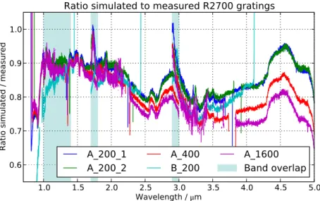
5.5.3 Overall instrument throughput . . . 83
5.5.4 IFU throughput . . . 86
5.6 Limitations of simulations . . . 87
6 NIRSpec science simulations 91 6.1 Multi-object deep field . . . 91
6.1.1 Introduction . . . 91
6.1.2 Observation scene creation . . . 91
6.1.3 Galaxy shapes . . . 92
6.1.4 Galaxy spectra . . . 97
6.1.5 Exposure simulation . . . 98
6.1.6 Spectrum extraction . . . 101
6.1.7 Results and discussion . . . 103
6.2 Exoplanetary transits . . . 106
6.2.1 Introduction . . . 106
6.2.2 Host star brightness limits . . . 108
Contents
6.2.4 Effective integration times . . . 113
6.2.5 Signals and noise . . . 114
6.2.6 Simulations of HD189733b . . . 120
6.2.7 Simulations of GJ1214b . . . 123
6.2.8 Simulations of an Earth-sized planet in the habitable zone . . . 126
7 Conclusion and outlook 129 A Additional images 131 A.1 Verification of the as-built optical model . . . 131
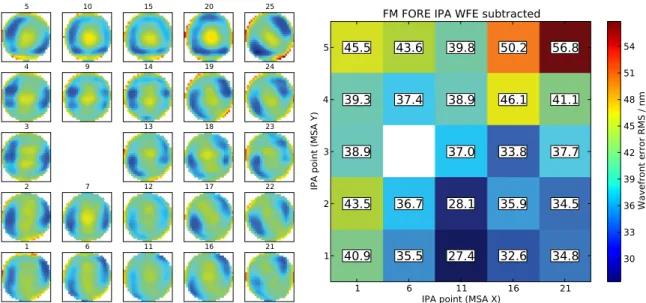
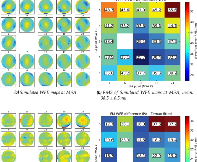
A.1.1 Measured wavefront errors at the FPA . . . 131
A.1.2 Simulated wavefront errors at the FPA . . . 133
A.1.3 Wavefront error residuals at the FPA . . . 134
A.2 NIRSpec model data . . . 136
A.2.1 Wavefront error maps . . . 136
A.2.2 Efficiencies . . . 138
B Publications 145 B.1 Overview . . . 145
B.2 Verification of the IPS with demonstration model data . . . 146
B.3 First simulation of a JWST/NIRSpec observation . . . 158
C Acronyms 163
List of Figures
1.1 Image of the JWST . . . 2
1.2 JWST OTE optical scheme . . . 4
1.3 JWST field of view allocation . . . 5
1.4 NIRSpec paraxial layout . . . 6
1.5 NIRSpec schematic drawing . . . 7
1.6 Image of the NIRSpec FM1 . . . 8
2.1 Scheme of the coordinate transform formalism . . . 12
2.2 Coordinate transform behavior outside fit region . . . 15
2.3 Spectrum derivatives on the detector . . . 16
2.4 FFT matrix pixel indexing . . . 17
2.5 Axis orientations in Fourier transforms . . . 18
2.6 Pupil and field orientations in NIRSpec optical planes . . . 21
2.7 Measured and simulated PSF at MSA . . . 22
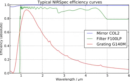
3.1 Exemplary NIRSpec component efficiency curves . . . 28
3.2 JWST OTE model wavefront error . . . 32
3.3 Measured wavefront errors at MSA . . . 33
3.4 Residuals of wavefront errors at MSA without optimization . . . 34
3.5 Model wavefront errors at MSA and residuals . . . 35
3.6 MIRR positions for optical measurements at the FPA . . . 36
4.1 Scheme pf the simple input FOV . . . 45
4.2 NIPPLS spectrum extraction workflows . . . 51
4.3 Schemes of pixel grids in spectrum rectification . . . 56
5.1 CLS SR1 source spectrum . . . 62
5.2 Spectrum data of SLIT_A_200_2 with CLS SR1 and G140H . . . 63
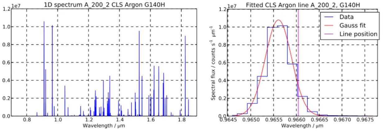
5.3 Spectrum data of SLIT_A_200_2 with CLS Argon and G140H . . . 64
5.4 G140H B_200 CLS flatfield spectrum . . . 66
5.5 G140H B_200 CLS flatfield trace data . . . 66
5.6 Extracted spectrum of SLIT_A_200_2 with CLS Argon and G140H . . 68
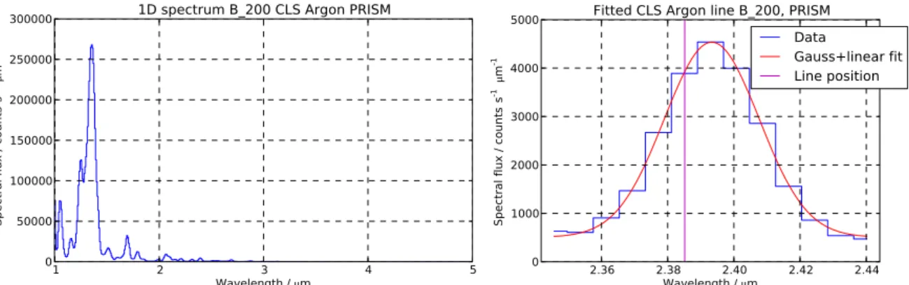
5.7 Extracted spectrum of SLIT_B_200 with CLS Argon and PRISM . . . . 69
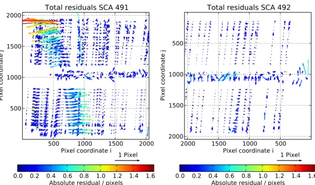
5.9 Total model fit residuals . . . 71
5.10 Residuals of Argon lines with G140H . . . 72
5.11 Residuals of Argon lines with G140H and GWA tilt . . . 74
5.12 Drawing of the CLS . . . 76
5.13 CLS PSB output spectra comparison . . . 78
5.14 CLEAR filter spectra with PRISM . . . 80
5.15 Relative transmission of F170LP measured and simulated . . . 81
5.16 Ratio of G235M and G235H spectrum and model data . . . 82
5.17 Ratio of IPS data to measured, R2700 gratings . . . 83
5.18 Ratio of IPS data to measured with tuned model . . . 84
5.19 Ratio of IPS data to measured, relative IFU spectra . . . 87
5.20 Scheme of the NIRSpec MULTIACCUM readout . . . 89
6.1 Evolution of galaxy sizes with redshift . . . 93
6.2 Sizes of galaxies in MOS simulation scene . . . 94
6.3 Sérsic profile curves with n“ 1 . . . 95
6.4 Integrated intensity of elliptical Sérsic sapes . . . 96
6.5 Galaxy contour images with MSA slitlet overlay. . . 96
6.6 Parameters of MOS simulation scene objects. . . 98
6.7 Exposure of the MOS simulation . . . 100
6.8 Images of two spectrum extraction steps . . . 102
6.9 Comparison of input and extracted galaxy spectra . . . 104
6.10 Scheme of exoplanetary transit events . . . 107
6.11 Map of losses in the A_1600 slit with G235H . . . 111
6.12 Photometric drift noise in the A_1600 slit with G235H . . . 112
6.13 Input spectrum of HD189733 . . . 120
6.14 Maximum electron rate for HD198733 . . . 121
6.15 SNR of primary transit of HD198733b . . . 122
6.16 SNR of atmospheric height of HD198733b . . . 123
6.17 SNR of emitted flux of HD198733b . . . 123
6.18 Input spectrum of GJ1214 . . . 124
6.19 SNR of atmospheric height of GJ1214b . . . 125
A.1 Measured wavefront errors at FPA center . . . 131
A.2 Measured wavefront errors at FPA`x-side . . . 132
A.3 Measured wavefront errors at FPA´x-side . . . 132
A.4 Simulated wavefront errors at FPA center . . . 133
A.5 Simulated wavefront errors at FPA`x-side . . . 133
A.6 Simulated wavefront errors at FPA´x-side . . . 134
A.7 Wavefront errors residuals at FPA center . . . 134
A.8 Wavefront errors residuals at FPA`x-side . . . 135
List of Figures
A.10 IPS model FORE and COL wavefront errors . . . 136
A.11 IPS model CAM wavefront errors at FPA center . . . 137
A.12 IPS model CAM wavefront errors at FPA `x-side . . . 137
A.13 IPS model CAM wavefront errors at FPA ´x-side . . . 138
A.14 IPS model mirror throughput . . . 138
A.15 IPS model FWA element efficiencies . . . 139
A.16 IPS model GWA element efficiencies . . . 141
A.17 IPS model detector QE . . . 143
List of Tables
1.1 NIRSpec basic characteristics . . . 3
2.1 Minimum required wavefront sampling . . . 25
3.1 Differences in raytracing coordinates . . . 38
4.1 Science input interface object file types . . . 47
4.2 Spatial source separation criteria . . . 49
4.3 Spectral source separation criteria . . . 49
5.1 Model fit residuals on the detector . . . 72
5.2 Ratio of simulated and expected electron rates . . . 75
6.1 Limiting minimal magnitudes of stellar spectra . . . 110
6.2 Mean drift noise in short exposures in the A_1600 slit . . . 113
6.3 Exposure parameters for observations of GJ1214 . . . 125
6.4 Exposure parameters for observations of G1214 put at 10 pc . . . 127
6.5 SNR of atmospheric features of an Earth-sized planet orbiting a M4.5 dwarf . . . 128
For NASA, space is still a high priority.
Dan Quayle
1
Introduction
1.1 The James Webb Space Telescope
Ideas and plans for a successor mission to the Hubble Space Telescope (HST) already date back to the early 1990s. In the wake of discoveries made with the HST, the astronomical community realized the need and potential of follow-up observations in the infrared (IR) wavelength range, especially to enable the research of redshifted objects, and to peek through dust clouds surrounding stars and star-forming regions.
These considerations led to the project of the James Webb Space Telescope (JWST, Gardner et al., 2006), a cooperation between the National Aeronautics and Space Administration (NASA), the European Space Agency (ESA), and the Canadian Space Agency (CSA). It is a large near- and mid-infrared space observatory with a primary mirror diameter of about 6.5 m (see Figure 1.1), and passively cooled to less than 50 K. The JWST will be placed in an orbit around the Sun-Earth Lagrange point L2 with an Ariane 5 launch foreseen in 2018. The observatory will carry a package of four science instruments: A Near-IR Camera (NIRCam, Horner and Rieke, 2004), a Near-IR Spectrograph (NIRSpec, Bagnasco et al., 2007), a Near-IR Imaging Slitless Spectrograph (NIRISS, former TFI, Doyon et al., 2010), and a Mid-IR Instrument (MIRI, Wright et al., 2010). The three near-infrared instruments will observe in a wavelength range of 0.6 to 5 μm, while MIRI is sensitive between 5 and 27 μm. The scientific objectives of the JWST mission can be split up into four themes:
• The end of the dark ages: first light and reionization • The assembly of galaxies
• The birth of stars and protoplanetary systems • Planetary systems and the origins of Life
In combination with NIRISS, there is also the Fine Guidance Sensor (FGS) to track the telescope pointing.
Figure 1.1: Image of the James Webb Space Telescope (credit: NASA).
1.2 Overview of the NIRSpec instrument
The primary science driver for NIRSpec is the spectroscopy of high-redshift galaxies out to z“ 6 and beyond, where the end of the dark ages and begin of the reionization era is assumed. A second objective is the study of the evolution and assembly of galaxies throughout the ages. Therefore, the instrument has been designed as a multi-object spectrograph with the goal to observe at least 100 multi-objects simultaneously. This capability is offered by a MicroShutter Array (MSA), consisting of four configurable grid masks for individual target selection (Kutyrev et al., 2008), covering a Field Of View (FOV) of at least 9 arcmin2. In addition, NIRSpec harbors an Integral Field Unit (IFU, Closs et al., 2008) with a small FOV to resolve single objects in both spatial and spectral dimensions. And lastly there are five FiXed SLits (FXSL) with different widths for high-contrast long-slit spectroscopy. Especially one of them (SLIT_A_1600) has gained scientific importance, as it offers the spectral analysis of exoplanetary transit events, and thus the characterization of exoplanets.
NIRSpec is sensitive across a spectral range of 0.6 to 5 μm, more than three wavelength octaves, which therefore is divided into three main scientific bands. In each of them, two dedicated gratings provide a spectral resolution of R“ λ{∆λ « 1000 and R « 2700. The complete wavelength span can also be observed with a
1.2 Overview of the NIRSpec instrument
Table 1.1: NIRSpec basic characteristics
Feature Value and explanation
Spectral range 0.6 μm–5.0 μm Field of view ą 9 arcmin2 Spectral resolutions R« 100 (low) R« 1000 (medium) R« 2700 (high) Spectral bands (gratings) Band I (1.0 μm–1.8 μm) Band II (1.7 μm–3.0 μm) Band III (2.9 μm–5.0 μm) Band 07 (0.7 μm–1.2 μm)
Filters CLEAR (complete range)
F100LP (1.0 μm–5.0 μm, long-pass) F170LP (1.7 μm–5.0 μm, long-pass) F290LP (2.9 μm–5.0 μm, long-pass) F070LP (0.7 μm–5.0 μm, long-pass)
F110W (0.99 μm–1.2 μm, target acquisition band-pass) F140X (0.8 μm–2 μm, target acquitision band-pass)
OPAQUE (closed, internal calibration and pupil reference) MSA elements Four quadrants of 365×171 microshutters, width 200 mas Fixed slits SLIT_A_200_1, SLIT_A_200_2, SLIT_B_200: width 200 mas
SLIT_A_400: width 400 mas
SLIT_A_1600: square aperture, width 1600 mas IFU 30 slices, widths 100 mas, lengths 3 arcsec GWA
elements
PRISM (R« 100)
G140M, G235M, G395M: gratings R« 1000, bands I-III G140H, G235H, G395H: gratings R« 2700, bands I-III TAM: Target Acquisition Mirror
Detectors 2 Mercury-Cadmium-Telluride (MCT) Sensor Chip Arrays (SCAs), each 2048ˆ 2048 pixels of 18 μm×18 μm
(100×100 mas2), labeled 491 (blue side) and 492 (red side)
prism at low resolution (R « 100). A list of all filters and dispersers and other details is given in Table 1.1.
NIRSpec is largely manufactured from Silicon Carbide (SiC), a ceramic which is very lightweight yet stiff, has a small thermal expansion, and is able to be optically
polished. Only some subsystems employ other materials as Invar and Aluminum. NIRSpec will be operated at a temperature of about 35 K.
1.3 Optical layout of JWST and NIRSpec
The JWST observatory consists of an Optical Telescope Element (OTE), and an Integrated Science Instrument Module (ISIM). The OTE primary mirror is assembled from 18 partially deployed hexagonal segments. The telescope optics has an effective focal length of 131.4 m and delivers a f{20 beam to the instruments at the curved exit focal surface (OTE Image Plane, OTEIP, see Figure 1.2). The field of view is split up into different regions for the science instruments and the FGS (Figure 1.3). JWST has an off-axis telescope, therefore a master chief ray has been defined serving as reference origin for the FOV coordinates. NIRSpec has a field allocation rotated clockwise by 41.5°, defined by nine field points F1–F9. The spectral direction is tangential to the symmetry axis of the telescope optics.
T ertiar y Mi rror OTE ISIM Cassegrain focus (V1, V3) origin f/#: 20.0
Effective Focal Length: 131.4 m
PM diameter = 6.6 m (circumscribed circle) V3 (anti-spacecraft) V1 V2 Focal Surface Primary Mirror Secondary mirror Fine Steering Mirror
Figure 1.2: Optical layout of the JWST telescope (from Gardner et al., 2006).
At the OTEIP, the NIRSpec Field Stop (FS) constrains the observable sky area. The light is then picked up by the two coupling mirrors COM1 and COM2 and guided to the optical bench. The general optical design consists of three major blocks, all employing Three-Mirror Anastigmats (TMAs) (te Plate et al., 2005). Figure 1.4 shows the paraxial representation of the optical train with the different modules and key components. A design drawing of NIRSpec with the light path can be seen in Figure 1.5.
The FORE optics re-images the OTEIP onto the slit plane at the MSA with an adjusted scale, a telecentric beam, and flattened focal surface. The nominal f-number
1.3 Optical layout of JWST and NIRSpec
Figure 1.3: Field of view allocation of the JWST instruments and elements of the NIRSpec
slit plane on the sky. The area for NIRSpec is rotated clockwise by 41.5° and defined by the nine points F1–F9.
is converted to f{12.5. In the pupil plane, the Filter Wheel Assembly (FWA) is located, carrying the filters listed in Table 1.1. Before reaching the MSA, the light also passes through the Refocusing Mirror Assembly (RMA), which allows the adaption of the focus without displacing the beam laterally.
The COLlimator optics (COL) projects the light from the slits onto the Grating Wheel Assembly (GWA), where a pupil plane is located. The GWA is equipped with eight elements described in Table 1.1 and allows the selection of disperser band and resolution, or mirror for imaging. Finally, the CAMera optics (CAM) focuses the (dispersed) beam onto the two detectors in the Focal Plane Array (FPA) with a f-number of f{5.6.
The IFU entrance aperture is located in the MSA plane, but normally obscured by the MSA magnet arm. IFU and MSA observations are exclusive as their spectra share the detector area, so all shutters have to be closed during IFU operations, and the IFU has to be blocked for MOS exposures. The IFU optics are split into an IFU FORE part, which re-images and -scales the MSA plane onto the slicer, and an IFU POST part, which picks up the 30 image parts, and creates a virtual slit image for each slice at the MSA plane. The rest of the light path is similar to the other observation modes. More details of the optical properties are given by Closs et al. (2008).
For the internal calibration, NIRSpec is equipped with a CAlibration Assembly (CAA), which hosts a series of lamps for different flatfield and spectral calibration illuminations. The beam of the CALibration optics (CAL) is coupled into the nominal NIRSpec path by putting the OPAQUE filter, that also acts as a shutter for external light.
One part of the ground support equipment is the Calibration Light Source (CLS, Bagnasco et al., 2008). This is the primary tool for the absolute radiometric and
OTE FORE COL CAM OTE primary FWA pupil GWA pupil
OTEIP MSA FPA
f /20 f /12.5 f /5.6 Slicer IFU entrance IFU virtual slit
IFU FORE IFU POST
Figure 1.4: Paraxial layout of the NIRSpec optical train with the main modules and nominal
focal ratios. Pupil stops are red, focal planes blue. The system pupil stop is the OTE primary mirror, the system field stop is located at the OTEIP. The IFU optics is coupled into the beam at the MSA focal plane.
spectral calibration of NIRSpec during the ground calibration campaigns. It consists of a lightbox with filament lamps and a set of four filter wheels, which carry different attenuators and spectral filters to generate appropriate illuminations for the flatfield and spectral calibration. In addition, there is an Argon emission line source and a laser diode for accurate spectral reference. All the sources are fed into a large integrating sphere, whose exit aperture mimics the JWST pupil. A Field Stop Mask (FSM) can be placed at the NIRSpec entrance for a flatfield illumination, as well as a PinHole Mask (PHM) to calibrate the geometrical distortion. The latter has a grid of small holes (diameters typically ă 8 μm) which create quasi point-like sources in the OTEIP, and also allow the characterization of the polychromatic PSF of the instrument.
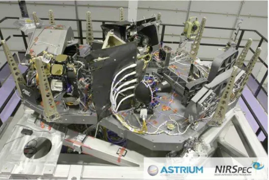
In spring 2011, the first NIRSpec flight model (FM1, Figure 1.6) has successfully undergone cryogenic testing and calibration. Due to hardware issues, a second assembly of the components is currently under way (FM2), and will likely be completed towards the end of 2012.
1.4 The NIRSpec Instrument Performance Simulator
Early in the development of NIRSpec, the need for an instrument simulator was realized, given the inherent complexity of a multi-object spectrograph, with all other operation modes on top. In the frame of the project, the Centre de Recherche Astrophysique de Lyon (CRAL) has developed the NIRSpec Instrument Performance
1.4 The NIRSpec Instrument Performance Simulator
Figure 1.5: NIRSpec schematic drawing with light path, top view. The light enters at
top right, passes through the FORE optics, the filter wheel, the RMA, and reaches the MSA slit plane. Proceeding through the collimator, it arrives at the grating wheel, then passes the camera, ending up at the detector (hidden in the CAM housing). (Credit: EADS/Astrium)
Simulator (IPS) software (Gnata, 2007; Piquéras et al., 2008, 2010). Its primary functions are to assess the instrument specifications, verify the performance, and do end-to-end simulations of calibration and scientific exposures. Besides, it serves to create realistic input data for processing tools, as the Instrument Quick Look Analysis and Calibration software (IQLAC, Gerssen et al., 2008) or the final NIRSpec data reduction pipeline.
To simulate the propagation of light, the instrument is divided into optical mod-ules, mostly defined by the single TMAs (COM + FORE, COL, CAM, CAL, OTE, IFU FORE, IFU POST), and the functional parts as filters, slits, and dispersers. The IPS uses a novel approach combining Fourier optics for the diffractive effects, geo-metrical coordinate transforms between the key optical planes, and simple efficiency calculations for the radiometry. These elements produce noiseless electron rates as a first main simulation product. The data contains the number of electron per second in each detector pixel, without any photon or readout noise, separate for each disperser order.
Figure 1.6: Fully assembled NIRSpec flight model 1 without the instrument cover (credit:
EADS/Astrium).
In a second stage, the readout process is simulated. All detectors in JWST use a sampling up the ramp-technique, where the signal in each pixel is probed non-destructively during the integration time. In the IPS, the electron rates for each pixel are collapsed over the orders, dark current is applied, and all the noise contributions added (Poisson, readout, etc.). The currently integrated signal is then put into a readout frame, and depending on the parameters, the frames are averaged to groups and written into the readout cube file.
In order to reduce the calculation time of electron rates, the sources are split into three spatial and spectral categories, each of them simulated differently. The spatial types are point sources (spatially unresolved), background sources (spatial variations on scales much larger than the instrument Point Spread Function, PSF), and extended sources (in between). The spectral types are continuum spectra (spectral variations on scales much larger than a resolution element), unresolved emission lines and absorption lines associated with a continuum, and spectrally resolved (in between).
Point sources are always completely Fourier-propagated for each required wave-length. For the other source types, there is a collection of pre-calculated PSFs for the step up to the slit plane, and for the spectrograph from slit to detector. They can be created with a single wavefront error map for the whole module, or with a grid of 3×3 maps covering the relevant fields. From them, the locally vaild PSF is then interpolated. Background sources are projected to the detector, the slit mask is applied, and they are convolved with the spectrograph PSF. Extended sources are
1.5 Goal and structure of this thesis
similarly processed, but convolved with the PSF at the slit plane before applying the slit mask.
In the case of emission and absorption lines, this is done for the single given wavelength only. With continuum spectra, the spectrograph PSF is collapsed in spectral direction before being interpolated to the local wavelengths. Besides, the sampling along the spectral direction on the detector is reduced to full pixels. The spectrally resolved spectra are always using the full 2D PSF for each oversampled wavelength step on the detector.
1.5 Goal and structure of this thesis
The goal of this thesis is to demonstrate the verification of the IPS, the instrument model and the instrument itself, and show first scientific simulations of NIRSpec observations.
In order to assure correct and accurate simulation results, one has to differentiate between two sources of errors: The intrinsic design of functions and algorithms in the software, and the data used in the instrument model.
The first can be partially checked by simulations with controlled inputs and models, which allow an independent calculation of the expected results. This approach has been taken in the acceptance tests required before the software delivery. However, they may not be sensitive to wrong assumptions in the software design, and effects caused by realistic model data.
The second type of errors can be mitigated by assembling the instrument model from measured and as-built subsystem data where possible. Nevertheless, this is not always feasible, the data may be inaccurate, and the interplay with other model data can cause unforeseen effects. To verify the software functions as well as the models, it is necessary to compare simulations with theoretical results and with real instrument measurements. A first set of them for the NIRSpec FM1 is available from the cryogenic calibration campaign, taken in spring 2011.
The final purpose of the IPS is to provide realistic simulations of in-orbit ob-servations. Naturally, a complex instrument also yields a complex simulator, and to facilitate the scientific application, it is necessary to create a simple way to use external source data. Besides, the IPS outputs are electron rates or raw data cubes, which need to be processed before any scientific analysis.
With the necessary tools and data prepared, it is then possible to produce accurate on-sky simulations, and analyze them easily. This enables a in-depth assessment and verification of NIRSpec’s capabilities for different science cases. Besides, it shows the characteristics and quality of the data that could be expected from the instrument.
This thesis describes the different steps in the model preparation and verification process, along with software tools for science data input and output data processing, and presents first simulations of on-sky observations. The structure is split into the
following parts: In chapter 2 we revise two specific IPS algorithms, and in chapter 3 we describe the data of the as-built instrument model. We present two software tools to facilitate the usage of the IPS in chapter 4. In chapter 5 we demonstrate how we verified the instrument model by comparing simulations with calibration data, and finally in chapter 6 we show the simulation and analysis of two scientific observation types: a multi-object scene, assembled from high-redshift galaxies, and exoplanetary transit events.
The work was embedded in the NIRSpec project environment, and makes use of various other existing efforts, most notably the IPS software. For clarity, we repeat essential characteristics of the simulator in chapter 2, in detail the algorithm for coor-dinate transforms in the instrument. Using this concept, we re-implemented the slit tilt effect based on the presented analysis. Also the general algorithm of the Fourier propagation and the coupling with physical parameters was established during the software design, however it had never been verified with the real orientations and the process of stepping through the instrument principal planes. In the end, the corresponding code was fully revised with the new considerations from this thesis.
The assembly of an as-built instrument model described in section 3.2 was largely a team effort, especially as it was part of the deliverable package in the IPS project. However, the work leading to the optical as-built model presented in section 3.3, originates solely from this thesis. It only uses the existing alignment model from Astrium as a starting point, and was done independently of officially required activities.
Finally, the development of the auxiliary software, the verification of the instru-ment model data, and the scientific simulations are fully original work, contributions from collaborators are marked accordingly.
If debugging is the process of removing bugs, then programming must be the process of putting them in.
Edsger Dijkstra
2
IPS software verification
2.1 Introduction
As mentioned in section 1.4, the IPS consists of several modules to model different physical processes (Piquéras et al., 2008). The basic considerations for the design of the algorithms can be found in Gnata (2007). However, some points had not been defined in detail, and other effects were only apparent once realistic simulations were run. Two major issues are the geometrical coordinate transforms, especially the effect of the slit tilt, and the orientation and sampling of wavefront errors and PSFs. We therefore review two simulation elements, the implementation of coordinate transforms in section 2.2, and the Fourier propagation in section 2.3. Independent of these major points, there was always close support of the software development team during the IPS project, for various issues ranging from user interaction, finding and isolating errors in the computations, and testing so far unused functionality.
2.2 Revision of coordinate transforms
2.2.1 General formalism
Transform formulas
The coordinate transforms in the IPS use a paraxial transform between the principal planes, and on top a 2D distortion polynomial (Figure 2.1). The paraxial part of a forward coordinate transform is defined by the magnification factors along the output axes γxand γy, the rotation angle of the coordinate system ϑ, and the absolute
position of the input and output frame origin in the local coordinatespx0 in, y0 inq and
ϑ xin yin y0 in x0 in x0 out y0 out Input Output xp yp yout xout
Figure 2.1: Scheme of the coordinate transform formalism. The transform is a rotation of the
input pointpxin, yinq around the center with the coordinates px0 in, y0 inq and px0 out, y0 outq
in the input and output planes (green), and a scaling along the output axes, giving the paraxial output coordinatespxp, ypq. The distortion is added as a 2D-polynomial yielding
the output coordinatespxout, youtq (red). The rotation angle ϑ is measured anti-clockwise
from the output axes to the input axes. pxp, ypq are then calculated by
xp “ γx¨ rpxin´ x0 inq cospϑq ` pyin´ y0 inq sinpϑqs ` x0 out ,
yp “ γy¨ r´pxin´ x0 inq sinpϑq ` pyin´ y0 inq cospϑqs ` y0 out .
The optical distortion is applied in the form of a 2D polynomial of order n, so the final output coordinates of the transformpxout, youtq are
xout “ n ÿ i“0 n´i ÿ j“0 ai,jpλq xipyjp , yout “ n ÿ i“0 n´i ÿ j“0 bi,jpλq xipyjp .
The transmissive filters in the FORE cause a chromatic aberration, which is suffi-ciently fitted by first-order wavelength-dependent polynomial coefficients
ai,jpλq “ αx i,jλ` βx i,j , bi,jpλq “ αy i,jλ` βy i,j .
Other optical modules are only reflective, and their transforms therefore exhibit no chromatic dependence.
2.2 Revision of coordinate transforms
A backward transform is done in the reverse order. At first, the distortion is removed and the paraxial coordinates calculated:
xp “ n ÿ i“0 n´i ÿ j“0
ci,jpλq xouti yjout ,
yp “ n ÿ i“0 n´i ÿ j“0
di,jpλq xioutyoutj ,
where
ci,jpλq “ ρx i,jλ` σx i,j , di,jpλq “ ρy i,jλ` σy i,j . Then the input coordinates are
xin “ 1 γxpxp´ x0 outq cospϑq ´ 1 γypyp´ y0 outq sinpϑq ` x0 in , yin “ 1 γxpxp´ x0 outq sinpϑq ` 1 γypyp´ y0 outq cospϑq ` y0 in .
The presented approach is adjusted to the instrument in two ways: First, the polynomial order can be set to 1ď n ď 5 as this corresponds to the requirement for the design. Second, we also exploit the fact that there is no nominal rotation in the area where distortion occurs. The only place rotating the coordinates is between COM1 and COM2, which both are flat mirrors right after a focal surface, and do not change the optical behavior. Therefore it is allowed to put the rotation in the paraxial approximation, and adding the distortion in a single step.
Transform coordinates
The paraxial description of the optical modules is based on the nominal entrance and exit focal lengths. They can be different in both axes, so that in total four parameters fin x,y, fout x,y are present. For modules between a focal and pupil plane or reverse,
one of the focal length types is ignored.
In an image plane, the coordinates are the physical positions in the local refer-ence frame. For the transform between two image planes (as in the FORE), the magnification factors γx and γycorrespond to the ratio of the focal lengths:
γx “ fout x
fin x , γy “ fout y
fin y . (2.1)
In a pupil plane, the coordinates are angular values of the ray direction. Often they are given as direction cosines Γx,y,z, but we use a vector with unitary z-component
of the form ¨ ˝ x y 1 ˛ ‚“ ¨ ˝ Γx{Γz Γy{Γz Γz{Γz ˛ ‚
Between an image plane and a pupil plane, the magnification factors are then
γx“ 1
fin x , γy “ 1
fin y , (2.2)
and between a pupil plane and an image plane
γx “ fout x , γy “ fout y . (2.3)
2.2.2 Derivation of transform parameters
The transform parameters are calculated from raytracing data of the NIRSpec model in the ZEMAX® optical design software. For a set of wavelengths, a grid of points covering the field of interest is traced through each optical module, and the input and output coordinates are recorded. A priori the paraxial parameters are unknown, and a distortion fit is done with dummy paraxial values, the center coordinates px0in, y0inq, px0out, y0outq are set to the center of the data grid. Nevertheless, this
fit yields a valid transform calculation, which can be used to derive the paraxial parameters.
With the assumption that locally a paraxial approximation can be used, the parameters are related to the local derivatives as follows:
Bxout Bxin “ γx cospϑq, Bxout Byin “ γx sinpϑq, (2.4) Byout Bxin “ ´γy sinpϑq, Byout Byin “ γy cospϑq.
The derivatives can be calculated numerically for the center point, and by taking care of the signs, the magnifications and rotation of the average paraxial approximation are obtained with γy ě 0 and ϑ P r´π, πs. The new parameters are then put into
the transform, and a second distortion polynomial fit is performed, now based on a correct paraxial description.
From the new magnification factors, one can also derive the actual effective focal lengths with Equations 2.2, or 2.3. In the case of the FORE, where the transform is directly from focal to focal plane, another distortion fit is established between the OTEIP and FWA pupil plane to determine the effective entrance focal lengths. Then, the exit focal lengths are calculated with the module magnification and Equation 2.1. The described approach harbors the danger that the polynomials are only valid inside the grid area. Calculating a coordinate transform outside the defining grid
2.2 Revision of coordinate transforms
can lead to problematic results and has to be avoided, as it is evident in Figure 2.2. A partial solution is to slightly oversize the raytracing grids on the expected used area, or to choose a first order polynomial fit, which is more robust in the outside region. However, this corresponds to a paraxial system and is usually not sufficient to fit the optical distortion with the required accuracy, therefore it is only applicable in few cases.
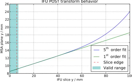
Figure 2.2: Behavior of the IFU POST coordinate transform for a slice at x“ 0 (slice center). The polynomial was fitted over a grid extended to y“ 7.2 mm, beyond the slice edge located at y“ 6 mm. The fifth order polynomial yields unrealistic distortion when using points farther away. A first order fit corresponds to a paraxial transform and is more robust in the outside region, but may generally not be sufficient to fit the distortion of the optics with the desired accuracy.
2.2.3 Slit tilt implementation
The previously illustrated recipe is capable of producing very accurate coordinate transforms for the OTE and inside NIRSpec. In all modules except the FORE optics, there is no or very little rotation, and no chromatic dependence of the coefficients. However, in combination with the dispersing element in the spectrograph, another effect occurs: the tilt of the slit image in the spectra.
In imaging mode, the spectrograph transform from slits to the detector can locally be approximated by a paraxial system. A slit itself may be rotated in the MSA plane by ϑrot, so that the spatial axis along the slit yslit and the MSA yMSA are not
collinear. The slit image will then be rotated by the angle ϑFPA` ϑrot. Assuming
ϑFPA“ ϑCOL` ϑCAM, and can be derived from the tilt of the MSA x-axis with ϑFPA“ ϑx “ arctanˆ ByFPA
BxMSA{
BxFPA
BxMSA
˙ , which is the same angle for the MSA y-axis
ϑy“ arctanˆ BxFPA ByMSA{ ByFPA ByMSA ˙ .
The local orientations are more complex in spectrographic mode, where the off-plane design of NIRSpec causes a curvature of the spectral lines (Schroeder, 2000, chapter 14). The curvature radius is very large compared to the length of a single slit, therefore it can be approximated with a slit tilt as shown in Figure 2.3. The single transforms for COL and CAM remain valid, but when including the disperser, the partial derivatives are not orthogonal any more, i.e. ϑx ‰ ϑy. The slit tilt is a
shear along the projected MSA x-axis by an angle ϑslit, which can be calculated as the difference between the tilts of the y- and x-axes to ϑslit “ ϑy´ ϑx. On the FPA,
the image of the slit is finally tilted by ϑy` ϑrot.
In the IPS this has consequences for all simulation types described in section 1.4, especially for continuum spectra. By collapsing the PSF in the FPA x-direction, all position information along this axis is lost and the resulting spectra would be straight in the FPA y-direction. The rotations of the distortion ϑxand the slits ϑrotare
typically much smaller than the slit tilt. Therefore the collapsed vector is rebinned along the x-direction with a shear rate of ∆xFPA“ ∆yFPAsinpϑy` ϑrotq, where ∆yFPA
is measured from the slit center trace location.
∂xMSA ∂yMSA λ = const ϑy ϑx ϑrot xFPA yFPA yslit =const
Figure 2.3: Scheme of the spatial derivatives and tilt angles on the detector. The slit is rotated
by ϑrot in the MSA plane. The derivatives along the MSA axesBxMSA and ByMSA are
not orthogonal. The spectra are curved due to the distortion, and the image of the slit is tilted by ϑy` ϑrot due to the off-plane spectrograph.
2.3 Revision of Fourier propagation
The PSFs for point sources are directly calculated on an oversampled grid of the detector pixels. To mimic a slit tilt, the slit mask is rotated by the angle relative to the orientation on the FPA ϑy` ϑrot. Extended and background sources are projected
onto the oversampled detector grid, and masked there with the slit shape. This mask is sheared in x with ∆xFPA“ ∆yFPAsinpϑslitq to introduce the slit tilt, and rotated by
ϑx` ϑrot to account for the geometrical rotation.
2.3 Revision of Fourier propagation
2.3.1 General application
The principle of propagating a wavefront from a pupil plane to an image plane and back is well known, and if the Fraunhofer approximation is valid, it can be numerically done with a Fast Fourier Transform (FFT) (Goodman, 1996). However, the relations between the orientation in physical coordinates in the optics and data arrays in the software require a careful definition of the algorithm and associated data input and output routines. NIRSpec has an unusual and rotated pupil shape, therefore the PSFs have a distinct appearance. Hence the PSF shape is an easy way to visually verify simulations with measurements, even though the absolute impact of a wrongly oriented PSF may be small.
2.3.2 Geometrical orientation
When using a FFT with a complex 2D array of the shape Nˆ N (FFT matrix, N even), the zero frequency component is associated with the center of a pixel. In the
Figure 2.4: Pixel indexing of a FFT matrix. The zero frequency is in pixelp1, 1q for the FFT
standard FFT output, this pixel is located in the corner of the array with indexp1, 1q (we use indices starting at 1). To enable the physical application of pupil apertures and wavefront error (WFE) maps, which generally have the coordinate frame center in the array center, the FFT matrix has to be transformed to put the zero frequency at pixelpN{
2` 1,N{2` 1q, and back for the FFT transform (see Figure 2.4). We generally
assume the zero frequency pixel to be in the center of the matrix.
The physical extent and orientation can be defined by auxiliary parameters. We associate a FFT matrix with the pixel step sizes of the array ∆x, ∆y and the physical position of the corner pixel p1, 1q, px0, y0q. In similar fashion, the model data as wavefront errors and pupil masks have their own physical coordinates. If they are provided in the instrument reference frames, and the FFT propagation keeps track of the physical coordinates, one obtains the PSFs with the correct orientation.
By default, the x- and y-axes in a Cartesian system span the input plane, while the z-axis points downstream along the propagation of the light (Figure 2.5). After a Fourier transform, the axes in the output plane are collinear to the input plane. For a propagation from pupil to pupil via image plane, an inverse FFT (iFFT)F´1 and a FFT F are done sequentially. In the mathematical definition, the coordinate systems remain collinear, while in the real optical system, the pupil content is flipped. In the IPS algorithm, this effect has to be traced by adjusting the physical parameters in the FFT matrix, and not flipping the array contents, which would otherwise move the pixels to wrong frequency coordinates.
z x y y y x x
Pupil plane Focal plane Pupil plane
F
−1 FFigure 2.5: Orientations of the coordinate axes in the Fourier propagation from pupil to pupil
via focal plane. The planes are spanned by x and y, z points along the propagation of the light. The propagation is calculated by an inverse and a forward Fourier transform F´1 andF. Mathematically the coordinates stay collinear, while the pupil is flipped optically.
2.3 Revision of Fourier propagation
2.3.3 Single propagation steps
Pupil to focal plane
If there is no previous propagation step, the complex FFT matrix in the pupil plane Appi, jq is initialized with 1 everywhere. The origin is in pixel pN{2` 1,N{2` 1q. The
physical step size ∆xp, ∆yp has to be chosen for appropriate sampling of the pupil
and PSF. In subsection 2.3.5 we describe this adjustment in detail. The physical position of pixel p1, 1q is given as
x0p “ ´ N 2∆xp
, y0p “ ´ N 2∆yp
.
At a specific wavelength λ, a wavefront error map Wpx, yq is then applied by interpolating the data at the physical coordinates of the FFT matrix pixelspxi,j, yi,jq, and changing the phase with
A1ppi, jq “ Appi, jq ¨ exp
ˆ
2πı Wpxi,j, yi,jq λ
˙ .
In similar fashion, a pupil intensity mask Ipx, yq, 0 ď Ipx, yq ď 1 is applied by changing the amplitude as
A2p “ A1ppi, jq ¨ Ipxi,j, yi,jq.
The WFE map does not influence the amplitude of the complex matrix, and therefore has to cover the same area of the pupil mask. Otherwise, no wavefront error is applied outside the available area while the intensity may be not zero. This can lead to wrong PSFs consisting of a combination of a degraded part with aberrations and an ideal PSF without.
The complex amplitude in the focal plane is the inverse Fourier transform of the pupil
Af “F´1pA2pq, and the pixel step size is now
∆xf “ λ fout x
∆xpN , ∆yf “
λ fout y
∆ypN (2.5)
with the exit focal lengths of the optical module fout x, fout y. Like before, the
coordinate of the corner pixel is x0 f “ ´ N
2∆xf , y0 f “ ´ N 2∆yf .
Focal to pupil plane
The Fourier propagation starting at a focal plane is only reasonable if there is a complex matrix Af present from a previous pupil-to-focal propagation. The amplitude in the pupil plane is then the FFT of the focal plane:
Ap“FpAfq.
As mentioned in subsection 2.3.2, the optical pupil is now rotated by 180°, while the Fourier matrix is not. Therefore the step and start values have to be inverted:
∆xp“ ´λ fin x ∆xfN , ∆yp “ ´ λ fin y ∆yfN , x0p “ ´ N 2∆xp , y0p “ ´ N 2∆yp .
This does not change the data, but relates the array correctly to the local coordinates. If another propagation step to a focal plane is necessary, the PSF there will be oriented the right way.
2.3.4 Implementation for NIRSpec
The Fourier algorithm uses the system of optical modules in the IPS (section 1.4). They are characterized with their pupil diameter D, and nominal entrance and exit focal lengths for both axes. These can be calculated with the scheme presented in subsection 2.2.2.
To define the orientations at the principal optical planes, we used the official NIRSpec optical model, where the reference frames in pupils and focal planes are given (Figure 2.6). We then put together the steps for a FFT-based propagation from one plane to the next, including the coordinate flips and rotations. We also noted the orientation of the z-axis, and how a wavefront with positive phase is oriented locally. This is important to correctly add the single WFE maps at different steps. We tested the newly assembled Fourier module using pupil masks with unique features to detect the orientations of pupils and PSFs. Comparing with a Python-based implementation, we could successfully reproduce the results in the IPS.
To verify the scheme with real instrument data, we used measurements taken during the NIRSpec Demonstration Model (DM) test campaign (Böker et al., 2010). With a pinhole mask at the NIRSpec field stop location, and the detector at the slit plane, the broadband PSFs of the FORE optics were recorded. In this configuration, the FWA stop defines the system pupil. In the DM, the stop is an oversized shape of the OTE primary boundaries, similar to the mask shown in Figure 2.6(b) without the three spider arms.
2.3 Revision of Fourier propagation
(a) Pupil orientation in the OTE pupil plane. Rotation to FWA plane: 180°+41.5°.
(b) Pupil orientation in the FWA and IFU FORE pupil plane. Rotation to GWA plane: 180°
(c) Pupil orientation in the IFU POST and GWA pupil plane.
(d) FOV orientation on the sky. Rotation to OTEIP plane: 180°.
(e) FOV orientation in the OTEIP. Rotation to MSA plane: 41.5°.
(f) FOV orientation in the MSA and IFU slicer plane. Rotation to FPA plane: 180°.
(g) FOV orientation on the FPA.
Figure 2.6: NIRSpec pupil and field orientation in various key optical planes with the projected
dispersion direction. The local physical axes are x to the right, y up. The z-axis points downstream except for the MSA and FPA planes. To move to the next plane, the data has to be rotated counterclockwise with the given angle.
One PSF example, reconstructed from dithered data as in Dorner et al. (2010, see section B.2), is shown in Figure 2.7(a). It is the polychromatic PSF of a pinhole in the spectrum range 0.9–1.9 μm. At this wavelengths, the FORE optics is already diffraction limited, therefore the PSF is purely determined by the pupil stop shape. Clearly visible is the six-spike diffraction pattern caused by the hexagon-like outer edge of the FWA stop.
For a comparison we simulated the monochromatic PSF of the FORE at 1.5 μm shown in Figure 2.7(b). The orientation of the diffraction spikes is the same, con-firming correct handling of the stop masks and FFT matrices. As the measured PSF contains contributions from longer wavelengths, the simulated PSF size is slightly smaller, but generally matches in the extension and decay of the diffraction features.
(a) Measured broadband PSF of the NIRSpec demonstration model at MSA in 0.9–1.9 µm
(b) Simulated FORE PSF at MSA at 1.5 µm
Figure 2.7: PSFs of the NIRSpec FORE optics. (a): Measured in the NIRSpec demonstration
model. (b): simulated with the IPS. The diffraction pattern is rotated alike. The PSF size is similar, the measured PSF is slightly larger as it contains contributions from longer wavelengths.
2.3.5 Sampling of PSFs and wavefront errors
Space domain
The physical pixel sizes of the FFT matrices are directly linked to each other (Equa-tion 2.5). It is therefore necessary to establish a rela(Equa-tion between the sampling of the PSF and the WFE maps. Considering only one dimension, we get
∆xf “ λ fout x ∆xpN “ λ f # N ¨ D ∆xp “ λ f # N ¨ np ,
where f #“ f {D is the focal ratio of the optical module, and npthe number of pixels
sampling the pupil in the FFT matrix.
In a PSF, the smallest structure present is of the size of the Airy disc, which has the radius rAiry “ 1.22λ f #. This also applies to speckles in aberrated systems. The sampling of the PSF can then be characterized by the number of pixels within one Airy radius, nx: nx “ 1.22λ f # ∆x f “ 1.22 N np .
This means that the sampling of the PSF only depends on the sampling of the pupil area and the size of the FFT matrix, independent of any optical parameters, and vice versa.
The pre-computed PSFs for non-pointlike sources are created with a constant nx.
2.3 Revision of Fourier propagation
varies spectrally as
∆xf “ 1.22λ f # nx .
In the case of point sources, the Fourier propagation is done for each PSF indi-vidually. To avoid spatial interpolation, the final PSF is sampled with the selected detector oversampling, and the initial step size is calculated accordingly. Therefore, ∆xf is constant, ∆xp changes with wavelength, and so do nx and np.
Frequency domain
In the PSF matrix, the pixel indices with respect to the origin are´N{2, ´N{2` 1, . . . ,
´1, 0, 1, . . ., N{2´ 2, N{2´ 1 with the PSF being centered at 0. The spatial frequency
coordinates of the pixels are ´N∆xN{2 p ,´ N{2 ` 1 N∆xp , . . . ,´ 1 N∆xp , 0, 1 N∆xp , . . . , N{2 ´ 2 N∆xp , N{2 ´ 1 N∆xp .
The minimum spatial frequency resolved in the pupil is kmin “ 1
D “
1 np∆xp ,
and the maximum frequency
kmax “
np{2
D “
1 2∆xp .
The index corresponding to the minimum frequency iminis given as
imin N∆xp “ 1 np∆xp and so imin “ N np .
The smallest reliable structure in the PSF extends then from´imin. . . imin , which is similar to the number inside the Airy radius nx. Therefore the minimum reliable
sampling in the PSF corresponds as expected to the Airy disc, which by definition is the smallest possible structure.
The index corresponding to the maximum frequency imax is then
imax “
N∆xp
2∆xp “
N 2 .
2.3.6 Required sampling for NIRSpec
Pre-computed PSFs
For a reasonable PSF sampling, the default values are N “ 2048 and nx “ 6, which
give np “ 416. The pre-computed PSFs are stored keeping only the central N{2-sized
array to prevent aliasing effects in the outer matrix area during the convolution of the detector images. At short wavelengths, the large relative WFE creates a large halo of scattered light in the PSF matrix. When cutting the central part, some intensity is lost and not recovered, as the final PSFs are normalized to total intensity of 1. This effect is stronger with smaller ∆xf and therefore larger nx. The default parameters
are a tradeoff between calculation speed, resolution of the PSF, the wavefront map, and errors in the normalization, but can be changed during the IPS model creation if the user considers other values as more appropriate.
When cutting the central part of the PSF matrix, it is important to have correct values out to˘N{4. According to section 2.3.5, the wavefront data then needs to be
resolved with nWFE ě np{2 “ 208. np remains as before, it only defines the size of
the pupil in pixels, not the real resolution of the data.
Point source propagation
The default FFT matrix size is N “ 2048, the oversampling factor 30, and ∆xf “
0.6 μm1. A very important aspect for point sources is the calculation of the slit losses. Especially to assess the photometric stability of exoplanetary transit observations, this has to be done with high accuracy. It means that the PSFs at the slit plane need to be valid at least out to the slit edges.
Considering a slit with the aperture size xS, yS being centered on the PSF, it covers
NSx “ xS ∆x f MSA , NSy“ yS ∆y f MSA
pixels. For simplicity, we do the calculation for one dimension. In the extreme case, where NSx “ N, the PSF matrix needs to be valid out to the edges, which requires the wavefront error to be resolved with
nWFE “ N∆xf MSA λ f #FORE out “
xS λ f #FORE out
pixels. In Table 2.1 we show exemplary values of nWFE for different slit types and
a shutter pattern. For a centered PSF to be accurate out to the slit edges at short wavelengths, the WFE diameter needs to be nWFE ě 193.
1It is possible to change the parameters for an electron rate computation by setting the oversampling
to 10, 20, or 40, and the point source FFT matrix size to 1024 or 4096, depending if the focus of the simulation is on speed or resolution of PSF and WFE structures.
2.3 Revision of Fourier propagation
Table 2.1: Minimum required wavefront sampling for valid PSF data in different slit
aper-tures.
Slit aperture nWFE
Name, axis xS oryS / mm λ “ 0.6 µm λ “ 5 µm 1x5 shutters, y 1.01 135 17 SLIT_A_200_1, y 1.27 169 21 SLIT_A_400, y 1.45 193 24 SLIT_A_1600, x 0.631 85 11 SLIT_A_1600, y 0.620 83 10
With the fixed PSF pixel size, the sampling in the GWA pupil plane is ∆xp GWA “ λ fCAM
∆x
fN
, and the spatial sampling in the MSA plane
∆xf MSA“ λ fCOL
∆xp GWAN “ ∆xf
f #COL f #CAM .
The sampling in the FWA pupil, where the Fourier propagation usually starts, is then
∆xp FWA “ λ fFORE out ∆xf MSAN .
The nominal focal ratios of the collimator and the FORE at the MSA are equal, therefore
∆xp FWA “ ∆xp GWA . The sampling of the PSF and the pupils is then
nx MSA “ nx ,
and because the nominal pupil diameters at FWA and GWA are equal np FWA “ np GWA .
With the camera focal ratio f #“ 5.6, the PSF sampling ranges from nx “ 6.8 . . . 57,
the pupil sampling from np “ 365 . . . 44 for the wavelengths λ “ 0.6 . . . 5 μm. This
is well balanced to sufficiently resolve both the PSFs at short wavelengths, and the wavefront errors at long wavelengths.