Determination of optimal conditions and kinetic rate parameters in continuous flow systems with dynamic inputs

Determination of Optimal Conditions and Kinetic

Rate Parameters in Continuous Flow Systems with

Dynamic Inputs

by

Kosisochukwu C. Aroh

B.S., University of Maryland (2012,2013)

S.M., Massachusetts Institute of Technology (2015)

Submitted to the Department of Chemical Engineering

in partial fulfillment of the requirements for the degree of

Doctor of Philosophy

at the

MASSACHUSETTS INSTITUTE OF TECHNOLOGY

@

Massachusetts Institute of Technology 2018. All rights reserved.

Signature redacted

A u th or ...

...

S

PfApartment of Chemical Engineering

December

20, 2018

ignature redacted

Certified by.

-rren K.

Klavs F. Jensen

Lewis Professor of Chemical Engineering

Thesis Supervisor

Accepted by ...

Signature redacted

MASSACUTT ILNSTITUTE

OF TECHNOLOGY

MAY 1

6

2019

LIBRARIES

Patrick S. Doyle

Chairman, Committee for Graduate Students

77 Massachusetts Avenue

Cambridge, MA 02139

MfTLibraries

DISCLAIMER NOTICE

Due to the condition of the original material, there are unavoidable

flaws in this reproduction. We have made every effort possible to

provide you with the best copy available.

Thank you.

The images contained in this document are of the

best quality available.

Determination of Optimal Conditions and Kinetic Rate

Parameters in Continuous Flow Systems with Dynamic Inputs

by

Kosisochukwu C. Aroh

Submitted to the Department of Chemical Engineering on December 20, 2018, in partial fulfillment of the

requirements for the degree of Doctor of Philosophy

Abstract

The fourth industrial revolution is said to be brought about by digitization in the manufacturing sector. According to this understanding, the third industrial revolu-tion which involved computers and automarevolu-tion will be further enhanced with smart and autonomous systems fueled by data and machine learning. At the research stage, an analogous story is being told in how automation and new technologies could rev-olutionize a chemistry laboratory. Flow chemistry is a technique that contrast with traditional batch chemistry in one aspect as a method that facilitates process au-tomation and in small scales, delivers process improvements such as high heat and mass transfer rates. In addition to flow chemistry, analytical tools have also greatly improved and have become fully automated with potential for remote control.

Over the past decade, work utilizing optimization techniques to find optimal con-ditions in flow chemistry have become more prevalent. In addition, the scope of reactions performed in these systems have also increased. In the first part of this thesis, the construction of a platform capable of performing a wide range of these reactions on the lab scale is discussed. This platform was built with the capability of performing global optimizations using steady state experiments. The rest of the thesis concerns generating dynamic experiments in flow systems and using these conditions to gain more information about a reaction.

The ability to use dynamic experiments to accurately determine reaction kinetics is first detailed. Through these experiments we found that only two orthogonal exper-iments were needed to sample the experimental space. After this an algorithm that utilizes dynamic experiments for kinetic parameter estimation problems is described. The approach here was to use dynamic experiments to first quickly sample the de-sign space to get a reasonable estimate of the kinetic parameters. Then steady state optimal design of experiments were used to fine tune these estimates. We observed that after initial orthogonal experiments only three more conditions were needed for accurate estimates of the multi-step reaction example.

In a similar fashion, an algorithm for reaction optimization that relies on dynamic experiments is also described. The approach here extended that of adaptive response

surface methodology where dynamic orthogonal experiments were performed in place of steady state experiments. When compared to steady state optimizations of multi-step reactions, a reduction by half in time needed to locate the optimum is observed. Finally, the potential issues that arise when using transient experiments in automated systems for reaction analysis are addressed. These issues include dispersion, sampling rate, reactor sizes and the rate of change of transients. These results demonstrate a way with which technological innovation could further revolutionize the chemistry laboratory. By combining machine learning, clouding computing and efficient, high information experiments reaction data could be quickly collected, and the information gained could be maximized for future predictions or optimizations.

Thesis Supervisor: Klavs F. Jensen

Acknowledgments

Firstly, I would like to express my sincere gratitude to my advisor Prof. Jensen for the continuous support of my Ph.D study, for his patience, motivation, and immense knowledge. I honestly could not have made it through my PhD without his guidance. In addition to my advisor, I would like to thank the rest of my thesis committee: Prof. Jamison, Prof. Green, and Prof. Braatz, for their insightful comments and encouragement, but also for the hard question which pushed me to widen my research from various perspectives. Prof. Jamison was a co-advisor for one of the projects in this thesis. I would like to also thank him for making his laboratory and resources therein available for some of the work carried out in it.

I also extend my sincere thanks to other members of the molecules on demand

project. For all their work on setting up and running the chemistry required for this project, I would like to thank Dr. Anne-Catherine Bedard, Grace Russell and Dr. Aaron Bedermann of the Jamison Group. Anne-Catherine contributed significantly on this on this project. For their work on the design and construction of the system,

I would like to thank Dr. Andrea Adamo, Jeremy Torosian and Brian Yue. Andrea

contributed significantly and lcd this endeavor. I also want to thank Dr. Dale Thomas who was not part of the project but his work with pumps proved to be very useful.

I thank my fellow labmates for discussions, collaboration and group dinners over

the years. I specifically want to thank members of the chemical synthesis subgroup over the years: Dr Brandon Reizman, Isaac Roes, Dr. Milad Abolhasani, Dr. Stefano Lazzari, Dr. Gaurav Giri, Connor Coley and Yiming Mo. The discussions and work presented over the years have helped me develop a wider range of understanding and exposure to scientific \Work in the field of continuous flow chemistry.

Lastly, I would like to thank my family: my parents, my brothers and sister for supporting me throughout my life especially the last few years during this thesis. I have had personal struggles associated with and predating my PhD. For help through-out this time, I have relied on a few close friends, especially my girlfriend/fiancee, and to them I am grateful.

THIS PAGE INTENTIONALLY LEFT BLANK

Contents

1 Introduction and Motivation 23

1.1 System Identification . . . . 24

1.2 Design of Experiments and Optimization . . . . 26

1.3 System Identification in Chemical Processes . . . . 29

1.4 Overview of Thesis and Goals . . . . 36

2 MoD: An Automated Continuous Flow Platform for the Optimiza-tion and Synthesis of Lab-Scale Chemicals 37 2.1 Introduction . . . . 37

2.1.1 State of the Art in Automated Synthesis . . . . 38

2.2 System Components . . . . 40

2.2.1 R eactors . . . . 43

2.3 N ethod . . . .. .. . . ... ... . . . . 45

2.3.1 Optimization in oD. . . . . 45

2.4 Experim ental . . . . 51

2.4.1 Online Analysis and Optimization in MoD . . . . 52

2.4.2 Optimization to Substrate Scope in MoD . . . . 52

2.4.3 Complex Epoxidation Optimization and Kinetic Analysis in MoD 60 2.5 Results and Discussion . . . . 62

2.5.1 Online Analysis and Optimization in MoD . . . . 62

2.5.2 Optimization to Substrate Scope in MoD . . . . 64

2.5.3 Complex Epoxidation Optimization and Kinetic Analysis in MoD 72 2.6 Conclusion . . . . 76

3 Simultaneous Continuous Temperature and Flowrate Ramps for Ef-ficient Reaction Kinetics

3.1 New approach to reaction kinetics ...

3.2 Procedure for Modeling Dynamic Inputs ...

3.3 Efficient Kinetic Experiments of Paal-Knorr Reaction with Infrared Sam pling . . . . 3.3.1 3.3.2 3.4 Other 3.4.1 Experimental Method Results and Discussion Applications . . . . Complex Mechanims . . . 3.4.2 Mechanism Identification . 3.5 Conclusion . . . . 79 80 83 88 . . . . 8 8 . . . . 8 9 . . . . 9 5 . . . . 9 5 97 99

4 Foundation for Dynamic Kinetic Parameter Estimation mization Experiments

4.1 Introduction . . . .

4.2 M ethod . . . .

4.2.1 Space Sampling . . . .

4.2.2 Dynamic Experiments Methodology . . . . 4.2.3 D-Optimal Dynamic Kinetic Experiments . . . . .

4.2.4 Adaptive Response Surface Methodology . . . . 4.3 Experimental . . . . and Opti-101 . . . . 101 . . . . 102 . . . . 102 . . . . 106 . . . . 106 . . . . 109 . . . . 114

4.3.1 Parameter Estimation Dynamic Experiment Simulation . 4.3.2 Dynamic Optimization Experiment Simulations . . . . . 4.4 Results and Discussion . . . . 4.4.1 Parameter Estimation . . . . 4.4.2 Optimization . . . .

4.5 Conclusion . . . .

5 Applying Dynamic Optimization Ramps to Real Systems

5.1 Introduction . . . .

8

5.2 Dispersion . . . .

5.3 Sampling Rate . . . .

5.4 Simulated Dynamic Optimization of Suzuki-Miyaura Cross Coupling in MoD . . . . 5.4.1 Model Building . . . .

5.4.2 SNAr Dynamic Optimization . . . . 140

5.5 C onclusion . . . .

6 Conclusion and Future Direction

6.1 Summary of Contributions . . . .

6.2 Future Direction . . . .

A Vici M6 Pumps

B MoD User Interface

C Catalyst Monitoring fo Suzuki-Miyaura Reaction

D Kinetic Monitoring of Paal-Knorr Using Mass Spectrometer

E Space Sampling

F Dynamic Adaptive Response Surface Methodology

G Instructions for Matlab and LabVIEW files

9 131 138 139 139 143 145 145 148 151 153 155 157 161 165 169

List of Figures

1-1 System Identification framework[1] . . . . 25

1-2 Example Latin Hypercube Designs [2] . . . . 27

1-3 Comparing the optimal designs based on the confidence region around parameter estimates 01 and 02 [31 . . . ... . . . . 28

1-4 Local versus global maximum on a curve . . . . 28

1-5 Fed-batch fermentation reactor[41 . . . . 29

1-6 a) Automated microreactor flow setup for reaction optimization. b) Knoevenagel condensation of p-anisaldehyde and malononitrile cat-alyzed by 1,8-diazabicycl-[5.4.0]undec-7-ene (DBU). c)Optimization re-sults for Knoevenagel example using Simplex Method, SNOBFIT, and Steepest Descent Method. Objective function values are denoted by the color bar and range from 0 (poor) to 0.65 (good). Boundaries on the reaction variables are denoted by red dashed lines [5] . . . . 31

1-7 Maximization of the production rate of the Paal-Knorr reaction with different optimization strategies. The initial DoE of each trajectory is numbered. a) Steepest descent method. b) Conjugate gradient

method. c) Armijo conjugate gradient method.[6] . . . . 32

1-8 a)Optimization scheme for Suzuki-Miyaura cross-couplings in the pres-ence of 1,8-diazabicycl[5.4.0]undec-7-ene (DBU) and THF/water. b)

Conceptual diagram for automated Suzuki-Miyaura cross-coupling optimization[7,

1-9 a) Visualization of the Deep Reaction Optimizer (DRO) Model Un-rolled over Three Time Steps .b) a) Pomeranz-Fritsch Synthesis of Isoquinoline, (b) Friedlaander Synthesis of a Substituted Quinoline,

(c) Synthesis of Ribose Phosphate, and (d) the Reaction between

2,6-Dichlorophenolindophenol (DCIP) and Ascorbic Acid[9] . . . . 34

1-10 a) Model discrimination and parameter estimation of Diels-Alder

re-action. Weighted probability distributions of potential rate laws used for model discrimination calculations involved in selecting conditions for the 6th experiment. Experimental result is denoted by the arrow

110].b) Multistep reaction network for conversion of 2,4-dichloropyrimidine

to 4,4'-(2,4-pyrimidinediyl)bis-morpholine [111 . . . . 35

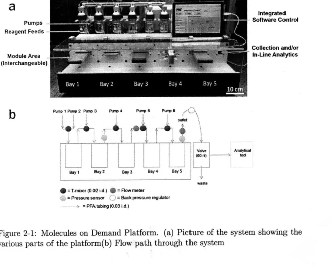
2-1 Molecules on Demand Platform. (a) Picture of the system showing the various parts of the platform(b) Flow path through the system . . . . 41

2-2 Calibration of IR sensors temperature measurement through the use of a therm ocouple . . . . 42

2-3 Description of analytical tools used inline with molecules on demand platform . . . . 44

2-4 All modules and dimensions . . . . 45

2-5 System optimization general method. (a) Optimization approach where each bay is treated independently and optimized in order from up-stream to downup-stream. (b) Optimization approach where the whole system is treated simultaneously . . . . 47

2-6 Relationship between system parameters and SNOBFIT algorithm . 48

2-7 Optimizing throughput of product in two setups that differ only in whether the first two pump flowrates are kept equal . . . . 49

2-8 Standard box and whiskers plot showing simulation results of the num-ber of experiments required to reach the optimum for the given sce-narios. The "+" represents outliers to the data, red represents the median of the data, blue represents a box around the lower quartile and upper quartile while the black represents the lowest and highest observation. (a) Two scenarios are compared for the optimization of a single step reaction with two inputs on different pumps to observe the effect of optimization setup on number of iterations. In scenario 1, the two inputs are allowed to vary independently and in scenario 2 they are constrained to the same value that is then allowed to vary. The second scenario had a median of 20 iterations while the first scenario needed more than forty experiments. (b) In the five cases, the number of iterations needed were compared for increasing number of reaction steps. Scenario 1 has only one reaction step, scenario 2 has two, up to scenario 5 having 5 reaction steps. Like in our system, every ad-ditional step has an adad-ditional reagent input. The median number of iterations required were used to understand how many iterations would

be needed in our system to find the optimum . . . . 50

2-9 Schematic of various system configurations inorder to understand the relationship between number of system parameters and iterations needed to find optimum using SNOBFIT algorithm . . . . 51

2-10 Legend for MoD reactor modules . . . . 52

2-11 Schematic of Paal-Knorr reaction in MoD system . . . . 53

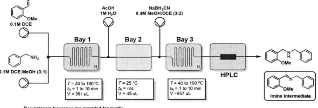
2-12 Schematic of reductive amination synthetic route . . . . 54

2-13 Schematic of Buchwald-Hartwig amination synthetic route . . . . 55

2-14 Schematic of Honer-Wadsworth-Emmons . . . . 56

2-15 Schematic of Suzuki-Miyaura . . . . 57

2-16 Schematic of SNAr reaction in MoD system . . . . 58

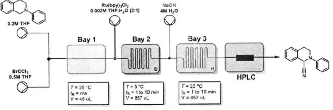
2-17 Schematic of photoredox generation of iminium . . . . 59

2-19 Schematic of epoxidation reaction . . . . 61

2-20 Schematic of epoxidation reaction with additives . . . . 62

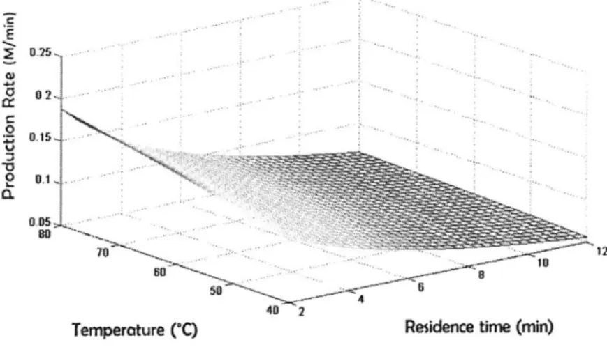
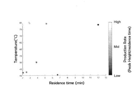
2-21 Response surface of production rate of Paal-Knorr reaction based on it's reaction kinetics . . . . 62

2-22 Production rate optimization of Paal-Knorr reaction via infrared spec-troscopy monitoring . . . . 63

2-23 Production rate optimization of Paal-Knorr reaction via HPLC moni-toring . . . . 63

2-24 Production rate optimization of Paal-Knorr reaction via mass spec-troscopy monitoring . . . . 64

2-25 Production rate optimization of Paal-Knorr reaction via Raman spec-troscopy monitoring . . . . 64

2-26 Substrate scope of the Buchwald-Hartwig reaction . . . . 65

2-27 Substrate scope of reductive amination reaction . . . . 67

2-28 Substrate scope of HWE reaction . . . . 68

2-29 Substrate scope of Suzuki-Miyaura reaction . . . . 69

2-30 Substrate scope of SNAr reaction . . . . 70

2-31 Substrate scope of Photoredox reaction . . . . 71

2-32 Substrate scope of ketene generation and 2+2 cycloaddition . . . . . 73

2-33 Quality of response surface models of epoxidation reactions . . . . 74

2-34 Response surface showing the relationships between variables of epox-idation reaction . . . . 75

2-35 Response surface showing the relationships between variables of epox-idation reaction . . . . 76

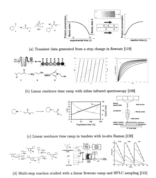
3-1 Summary of previous work in dynamic kinetic experiments with con-tinuous flow systems . . . . 81

3-2 Schematic of three different approaches for kinetic experiments. (a) Current steady state approach to collecting reaction concentration data over several temperatures and flowrates(b) Current dynamic approach of collecting reaction concentration data over several temperatures in flow. Flowrate is changed while the temperature is constant. (b) New proposed approach of a more efficient method of data collection. Both temperature and flowrate are changed simultaneous within the same experim ent . . . . 82

3-3 An example of how a batch of fluid is tracked based on when the mea-surement is taken and the details of the ramp method. The conditions that the batch of fluid underwent can then be calculated based on its history.. . . . .. . . . ... .. .. .. 85

3-4 Continuous flow microfluidic reactor setup . . . . 90

3-5 Concentration profile of 2 under temperature and residence time ramps. (a) Temperature ramp up experimental data (black circle), fitted model (dark line)(b) temperature ramp down experimental data (black cir-cle), fitted model (dark line) (c) temperature ramp up and down: tem-perature ramp down data (black circle), simultaneous fitted model-temperature ramp down (black line), model-temperature ramp up data (red circle), simultaneous fitted model-temperature ramp up (red line). . . 90

3-6 Constant temperature, residence time ramps. Model results of con-centration of 2 at 40'C (black), 60'C (red), 80'C (blue), 100'C (teal) (symbols). Experimental data of concentration of 2: 400

C (black),

60'C (red), 80'C (blue), 100'C (teal) (lines). (a) Residence time data

and fitted model. (b) Residence time data and temperature ramp down fitted model. (c) Residence time data and temperature ramp up fitted model. (d) Residence time data and simultaneous temperature ramp fitted m odel. . . . . 91

3-7 Residuals between models and concentration data. (a) Constant tem-perature model: temtem-perature ramp down (black), temtem-perature ramp

up (red). (b) Simultaneous temperature ramp model: temperature

ramp down (black), temperature ramp up (red). (c) Constant tem-perature model: 400C (black), 600C (red), 80'C (blue), 1000C (teal).

(d) Simultaneous temperature ramp model: 40'C (black), 600_{C (red),}

80'C (blue), 100'C (teal). . . . . 94

3-8 (i) Labelled reactor setup (ii) microreactor (iii) simulated temperature profile of microreactor (iv) simulated temperature profile of reactor with aluminium enclosure . . . . 95

3-9 Simulated kinetic data of esterification reaction with simultaneous tem-perature and residence time ramps. Kinetic data at 300C (red), 600C

(black) (line). Fitted model at 300C (red), 60'C (black) (circle). (a)

Control example in terms of reaction rate and ramp rates. (b) Fast re-action example with control ramp rates (c) slow rere-action with i) control temperature and residence time ramp rates and ii) control temperature ramp rate and slow residence time ramp rate (d) slow reaction with slow temperature ramp rate and slow residence time ramp rate. . . . 96

3-10 Comparison of simulated temperature and residence time ramps with

potential mechanisms. (red hollow) T ramp up (black hollow) T ramp down, (red filled) potential mechanism, T ramp up, (black filled) po-tential mechanism, T ramp down. Model (a) I, (b) II, (c) III, (d) IV . ... .... . . .. ... . . .. . . .. 99

4-1 Three different sine profile variations for two inputs . . . . 103

4-2 Conditions sampled in one reactor system with two flow rate inputs and one temperature using three different sine profile variations . . . 104

4-3 Conditions sampled in two reactor system with three flow rate inputs and two temperatures using three different sine profile variations . . . 105

4-5 Algorithm for the parameter estimation utilizing dynamic experiments 109 4-6 General procedure for adaptive response surface methodology . . . .111

4-7 General adaptive response surface methodology schematic for inte-grated dynamic experiments . . . . 113

4-8 Reactor system and corresponding reaction rate equations . . . . 115

4-9 One reactor system with corresponding reaction rate equations . . . . 116

4-10 Two reactor system with corresponding reaction rate equations . . . . 116

4-11 Initial results of parameter estimation procedure after dynamic exper-im ents . . . . 122

4-12 Sampled conditions at each iteration of the algorithm with correspond-ing response surface for a one reactor system. Green points(both light and dark) represent two new orthogonal ramps performed while blue corresponds to already performed experiments that were selected based on their high objective function value. The optimum was located using only three sets of ramps and four iterations of the algorithm . . . . . 126

4-13 Response surface of a two reactor system near the system optimum. Near the optimum the response surface becomes relatively flat making finding the optimum more challenging . . . . 127

4-14 Sampled conditions at each iteration of the algorithm with correspond-ing response surface for a two reactor system. Green points(both light and dark) represent two new orthogonal ramps performed while blue corresponds to already performed experiments that were selected based on their high objective function value. After four sets of ramps the design space was sufficiently reduced and one more iteration with pre-viously sampled conditions in this space confirmed the system optimum 128

5-1 Depiction of fluid being forced into a parabolic profile as it enters a tubular reactor. The diffusion, velocity and tube dimensions creates new forces in the fluid that change the effective diffusion coefficient of solute in the fluid . . . . . 132

5-2 Calculation of residence time distribution(RTD) for a non-ideal reactor. The RTD was then matched with an RTD of multiple CSTRs in series in order to get the CSTRs equivalent. E(O) =Tres * E(t), 0 - ' . . 134

'Tres

5-3 Series CSTRs compared an ideal PFR at various reaction conditions in order to demonstrate that adjusting the kinetic parameters of a first order reaction is not sufficient to get the results to match . . . . 134 5-4 One reactor setup with corresponding reactor volumes used to analyze

the dispersion in various labscale flow reactor. . . . . 135 5-5 Flowrate inputs for a one reactor system. The corresponding outlet

concentration and fitted model results based on the inputs is also shown 136

5-6 Measured outlet concentration with fitted model for various phase shifts between the two inputs of a Paal-Knorr reaction. . . . . 137 5-7 Measured outlet concentration with fitted model for various frequencies

of inputs of a Paal-Knorr reaction. A constant phase shift of pi/2 was used. For both the 230pL and 500pLL reactor, lowering the frequencies produced better agreement between the model and experiments. . . . 137 5-8 Measured outlet concentration with fitted model for the Paal-Knorr

reaction. lmL and 10mL were chosen to examine the effect of dis-persion in larger reactors. Although the 1mL reactor showed modest agreement, 10mL rcactor model was inaccurate during the first part of the experim ent. . . . . 138

5-9 A single reactor with two inputs accompanied by a 3 step reaction used

to compare the effects of various sampling rates. . . . . 139

5-10 SNAr reaction schematic for the MoD system . . . . 140

5-11 Comparison of the model of the objective function from the SNAT

reaction. A quadratic response model with flowrates and temperature as inputs were used to capture the behavior of the SNAr reaction . . 141

5-12 Procedure used to construct model of the SNAT reaction in the MoD

system. That model is then used as an encapsulation of actual exper-iments inorder to simulate the dynamic experexper-iments. . . . . 141

5-13 Dynamic inputs used for the first step of dynamic optimization of the

the SNA T. . . . .- - .. . . . . . . . . .. . . .142

5-14 Assuming a sampling interval of 30s, the measured data with fitted response surface . . . . 143

5-15 Assuming a sampling interval of 10 minute, the measured data with

fitted response surface . . . . 143

6-1 Future of automated flow synthesis. A combination of recent advance-ments in artificial intelligence, reaction databases and automated ex-perimentation has the potential to greatly transform the field of chem-ical synthesis . . . . 149

A-i Methanol in M6 pump . . . . 151

A-2 Water in M6 pump . . . . 151

B-i First page of the interface that displays the molecules taking place in the reactions . . . . 153

B-2 First page of the interface where the name of the reagents and modules of the system are entered . . . . 153

B-3 Second page of the interface where the details of the synthesis or opti-mization are entered . . . . 154

B-4 Third page of the interface where the various sensory measurements and setpoints are displayed . . . . 154

C-I Packing instructions for catalyst . . . . 155

C-2 Suzuki Miyaura cross-coupling reaction schematic . . . . 156

C-3 Graph of reaction conversion as a function of time. Over a five hour

D-1 Paal-Knorr reaction that occurs in the reactor. The protected propanol

amine does not participate in the reaction. When the reagents are sent to mass spectrometer, the ionization results in the deprotection of the propanol amine. This presents potential approach to generate a suitable inexpensive standard for flow reactions. . . . . 158 D-2 MS signal showing the for the Paal-Knorr reaction with a proponal

am ine calibrant . . . . 158 D-3 Kinetic results of using a similar molecule to calibrate the Paal Knorr

reaction in a mass spectrometer and comparing these results to that of the paal knorr reaction monitored with infrared spectrometer . . . . . 159

E-i One reactor system with two flowrate inputs and one reactor temperature162 E-2 Number of distinct conditions for various combinations of phase shifts

in the scenairios of a) regulur sine profiles, b) sine with changing fre-quencies and c) changing frequency and amplitude for a two reactor system . . . . 162 E-3 Two reactor system with three flowrate inputs and two reactor

tem-peratures .. . . . ... .. . .. . ... ... . .. . . . .. .. .163

E-4 Number of distinct conditions for various combinations of phase shifts in the scenairios of a) regulur sine profiles, b) sine with changing fre-quencies and c) changing frequency and amplitude for a two reactor system . . . . 163

List of Tables

2.1 Objective functions for Paal-Knorr optimization . . . . 53

2.2 Reductive amination optimization . . . . 54

2.3 Buchwald-Hartwig amination optimization parameters . . . . 55

2.4 Honer-Wadsworth-Emmons optimization parameters . . . . 56 2.5 Suzuki-Miyaura cross-coupling optimization parameters . . . . 57

2.6 SNAr optimization parameters . . . . 58 2.7 Photoredox generation of iminium optimization parameters . . . . 59 2.8 Optimization parameters for the ketene generation and 2+2 cycloaddition 60

2.9 Epoxidation optimization parameters . . . . 61

2.10 Buchwald-Hartwig amination optimized conditions . . . . 65

2.11 Reductive amination optimized conditions . . . . 66

2.12 Horner-Wadsworth-Emmons optimized conditions . . . . 67

2.13 Suzuki-Miyaura cross-coupling optimized conditions . . . . 68

2.14 SNAr optimized conditions . . . . 70

2.15 Photoredox optimized conditions . . . . 71

2.16 Ketene optimized conditions . . . . 72

2.17 Epoxidation optimized conditions . . . . 73

3.1 Fitting results of different potential mechanisms to temperature and residence time ramp data assuming a 3% error in concentration mea-surem ents . . . . 98

4.1 Correct parameters and bounds on potential estimates . . . . 114 4.2 System experiment conditions . . . . 114

4.3 Reaction parameters used in simulations . . . . 115

4.4 One reactor system experimental design space . . . . 116

4.5 Reaction parameters used in simulations . . . . 117

4.6 Two reactor system experimental design space . . . . 117

4.7 Flowrate and temperature ramps with corresponding response surface 119

4.8 Flowrate and temperature ramps with corresponding integrated pro-files as a function of sample number assuming a sampling rate of 30

seconds... ... 121

4.9 Parameter estimates after dynamic ramps and D-criterion optimal ex-perim ents . . . . 121 4.10 One Reactor Optimization Results . . . . 123

4.11 Two reactor optimization results . . . . 125

5.1 Equivalent number of CSTRs needed to produce a similar residence time distribution as non-ideal pfr . . . . 133 5.2 Estimated kinetic parameters from different sampling rates . . . . 139 5.3 SNAr optimization parameters . . . . 142

Chapter 1

Introduction and Motivation

The fourth industrial revolution, industry 4.0, is said to be brought about by digi-tization in the manufacturing sector[12]. According to this understanding, the third industrial revolution which involved computers and automation will be further en-hanced with "smart and autonomous systems fueled by data and machine learn-ing". The other components of industry 4.0 includes autonomous robots, simulation, horizontal and vertical system integration, industrial internet of things, cybersecu-rity, the cloud, additive manufacturing, augmented reality and finally big data and analytics[13]. This push to further incorporate these tools is highly desired for their potential impact on efficiencies and product quality.

The scale at which it makes sense to incorporate digitization is highly dependent on the specific industry. This goal of incorporating these technologies is not new the pharmaceutical industry. In 2002, the Food and Drug Administration (FDA) announced an initiative called Pharmaceutical Current Good Manufacturing Prac-tices(CGMPs) for the 21st century[141. The goal was to enhance and modernize the regulation of pharmaceutical manufacturing and product quality. This announcement renewed a focus on an old idea of quality by design in the industry. The concept fo-cuses on risk management with the relevant portions being process analytical tools (PAT) and continuous process verification. These improvements from a regulation stand point will require components of industry 4.0.

At the research stage, an analogous story is being told in how automation and

new technologies could revolutionize a chemistry laboratory. The process of carrying out chemistry research has largely not changed since the twentieth century. Many years are required to develop synthetic chemistry expertise and a significant amount of that time is spent 'setting up or cleaning apparatus, routine reaction optimization, repetition of trivial experiments, and scaling-up of well established procedures'[ 15]. Techniques that enhance automation and ability for more remote synthesis is well understood by most chemist to have the capabilities to revolutionize their work in terms of quality, quantity and scope[16].

Flow chemistry is a technique that contrast with traditional batch chemistry in one way as a method that facilitates process automation. In smaller scales, flow chem-istry also delivers process improvements such as better heat and mass transfer rates compared to traditional batch experiments[17]. Additionally because small amounts of reagents are used at a time in the milliliter and microliter size reactors; safety is enhanced as well in these systems. Due to these benefits, this technique has found more applications in the laboratory and industry 118, 19]. In addition to flow chem-istry, analytical tools have also greatly improved and become fully automated with potential for remote control[20].

The way these tools and techniques are combined to develop intelligent and fully automated systems is critical to their ultimate utility. Before automating a system and operating it at an optimal setpoint, an understanding of how the system operates is required. What follows is an overview of techniques that helps one understand how a system responds to various inputs and how these techniques have been utilized in continuous flow systems. Finally, the goals and contributions of this thesis in the area of system identification are summarized.

1.1

System Identification

System identification is the method of building a mathematical model that describes a system through the use of input and output data from said system. The method contains many topical areas, namely: experimentation, model structure, fit criterion,

Prior Knowledge Experilnmnt Data Model Setis CK: ooseit

Figure 1-1: System Identification framework[1J

model calculation, and evaluation. These areas are connected through the system identification loop in Figure 1-1111. This framework covers various areas of study, most notably: process control, parameter estimation, optimization and design of ex-periments. The applications vary from controlling a system process through specified inputs and outputs, fitting model parameters of a system model, optimizing con-ditions of a system through a model and understanding the relationships between system parameters and their effect on model output.

The focus of work outlined in later chapters will be on the experimentation and model calculation areas of system identification. The areas of model structure and determination of the correct model are other important topics that have been heavily discussed elsewhere[21, 22, 23, 24, 25, 26, 27, 28]. In those studies how one choses experiments that can elucidate the most probable model from a candidate of models are examined.

1.2

Design of Experiments and Optimization

Design of experiments (DOE) is a method of choosing samples in a design space in order to get the most amount of information using the minimum amount of re-sources/samples [2]. In this method there are trade offs between the number of sam-ples and accuracy of information collected. After a DOE, the next step is generally to process the information through Response Surface Modeling (RSM). The techniques that fall under RSM include linear, nonlinear, polynomial and stochastic methods. Generally interpolation or approximation techniques are performed to generate the specific type of model from the data samples.

Various designs ranging in properties have been proposed[29, 30], the most com-mon design being a full factorial where each parameter is broken into a predetermined number of levels and every combination of parameters based on these level are per-formed. In cases where many factors or levels exist, a fraction of the full factorial or block designs based on a primary factor(Randomized Complete Block Design) or a mix of factors (latin square) are performed. Another common design is the central composite where a full factorial number of experiments is performed but the 'star' experimental points are constructed based on distance from the central point. Other designs have been considered for cases where the resulting full factorial sample size would be too high such as Box-Behnken[31], Plackett-Burman[32] and Taguchi[33].

The designs mentioned so far have their foundation in statistics and trying to dif-ferentiate between parameter effects. Other sets of designs are focused on space filling of the experimental space. Though these designs are good for response surfaces, they are not level-based so it is generally not recommended for understanding interactions and main effects of parameters. Latin hypercube are a type of space filling design where the design space is divided into sub spaces, a subset of those sub spaces are then chosen such that the dimensions corresponding to the sub space do not correlate and finally within each of these sub volumes a random sample is taken to make up the actual design. An example of these designs for two and three parameters are shown in Figure 1-2.

(a) k =2. N =4 (b) k =3 N 3

Figure 1-2: Example Latin Hypercube Designs [2]

Optimal designs are another method of choosing new experiments to perform. Whether or not the design is optimal is dependent on what the goals of the experi-ments are. As mentioned before, when the goal is model discrimination an experiment is chosen based on the conditions that maximizes the differences in the expected model predictions[26, 21, 27, 28]. Another set of optimal designs are used when the goal is to generate more accurate estimates of a great model[23, 34, 3, 351. These set of designs focus on the sensitivity of responses to parameters and how these sensitivi-ties are combined with variance in parameter estimates in order to decide the next experiment. How some of the more common designs compare is shown in Figure 1-3. Less common optimal designs are detailed in other studies[36, 371.

As mentioned earlier, DOE-RSM is a way to process information from an exper-iment based on a predetermined evaluation criteria. Related to this problem, is the general field of optimization where the evaluation criteria is to minimize or maxi-mize some objective. DOE-RSM has been used to solve optimization problems and fall into the class of black-box optimizations, meaning information about the system other than its inputs and outputs is not used during the optimization. Various texts and resources detail other optimization routines and how they are organized[2]. An important distinction between types of optimizations is that of local and global opti-mization routines. Figure 1-4 depicts the difference between these two categories for the case of maximizations, namely local optimization routines identify any local

max-kopftaliy |Ellpse ofl

E-optimality

02

Figure 1-3: Comparing the optimal designs based on the confidence region around parameter estimates 01 and 02 [31

global maximum

Local maximum

-U

01

Figure 1-4: Local versus global maximum on a curve

imum while global optimizations identifies the only global maximum. Whether an optimization routine is local or global does depend on the assumption of the values of the objective function. In convex optimization it is assumed that the objective func-tion has only one extrema and hence finds the only local optima[38, 39]. Well known convex optimizations are gradient based routines such sequential quadratic program-ming and the conjugate gradient method. Generally global optimization methods find the global solution by dividing up the design space and performing local opti-mizations on each sub space before combining the solutions and arriving at the global optimal[40, 41].

time-varyingN inlputs

measured

responses

reaction

Figure 1-5: Fed-batch fermentation reactor[4]

1.3

System Identification in Chemical Processes

System identification in chemical processes has had a long history as mentioned ear-lier. During the time when the theory of design of experiments were developed, a com-mon example of a reaction system that was used to compare designs was the baker's yeast fermentation reactor model[42, 43, 44, 4, 45]. A schematic of the system is shown in Figure 1-5 with the governing equations of the process in Eqn. 1.3.1. In general the objective of this system was to design an experiment that yields the most information for the estimation of the parameters of the models. Asprey and Macchietto compared D-optimal, Worst-case (R-optimal), and expected value (ED-optimal) experimental designs[41. They concluded that the proposed R-optimal and ED-optimal reaction performed better(estimated parameters are closer to true parameter values) than the traditional D-optimal designs. The experiments designed in these systems were that of dynamic experiments of the experimental variables: substrate feed concentration(U2),

dilution factor(u1) and initial biomass concentration(xi).

dx

dt

reaction screening[46, 47, 48, 49, 501. Most of these systems were automated droplet system as apposed to continuous flow system. One of the earliest work in lab scale flow systems to incorporate optimization is that of Krishnadasan et al[51]. The synthesis of florescent CdSe nanoparticles was optimized using the SNOBFIT152] optimization algorithm. The setup consisted of two syringe pumps, one with CdO solution and the other with Se solution, that connects to a reactor with a controlled heating system. The effluent of the reactor flowed through a UV spectrometer before ending in up collection. The optimum intensity was optimized by adjusting the flowrates of the syringe pumps and the temperature of the reactor.

McMullen and Jensen constructed a flow system with an automated silicon mi-croreactor with syringe pumps, micromixer, online HPLC analysis, and tempera-ture control[5]. In this work, the Knoevenagel reaction between p-anisaldehyde and malonoitrile was used to compare the optimization of the product yield using three different optimization routines. From Figure 1-6, it can be seen for a two variable op-timization, residence time and temperature, of a simple reaction, the steepest descent method found the optimum conditions with the least amount of samples.

In a similar fashion, Moore and Jensen built an automated microreactor platform with online infrared spectrometer analysis in order to compare the optimization of various gradient based optimization routines[6]. The Paal-Knorr reaction was used in comparing steepest descent, conjugate gradient and Armijo conjugate gradient meth-ods. They were able to demonstrate the theory that incorporating an Armijo-type line-search increases the optimization efficiency of these gradient based algorithrnsl-7.

With the exception of SNOBFIT, the rest of theses algorithms mentioned so far are local optimization techniques. For simple reactions, this is sufficient but as more variables such as catalyst type and concentration with potential for deactivation are added, global routines would be required to find optimized conditions. In addition, cases where it is desired to screen and optimize reactions simultaneously have not been considered. Reizman et al. built an automated droplet flow platform in or-der to screen and optimize turnover number of the catalyst with an additional yield constraint or at least 90%[7]. The Suzuki-Myuara cross-couplings in the presence

IResidence time I

conentation con

t & Crtench

control Data acquisition I.

PRewcor 3 HeaterlCooler pMlxcr ISMI HPLO i Dilution Detection ..-.--- -...---....---.--- I

b

\/+

L

7~+

Objective function values

Figure 1-6: a) Automated microreactor flow setup for reaction optimization. b) Knoevenagel condensation of p-anisaldehyde and malononitrile catalyzed by 1,8-diazabicycl-[5.4.0]undec-7-ene (DBU). c)Optimization results for Knoevenagel exam-ple using Simexam-plex Method, SNOBFIT, and Steepest Descent Method. Objective function values are denoted by the color bar and range from 0 (poor) to 0.65 (good). Boundaries on the reaction variables are denoted by red dashed lines 15]

SteeestdesentAnn :ojuge

)tee m b)Conjugate gradient 0'1 0 _00 0 20210 1 2 2I 3 ... .

prtn t aSteepest descent cty-ivoa cobuate o

..'ao .. ...

5 0

10 1-2 ii. V0

- 40.6-

T-Figure 1-7: Maximization of the production rate of the Paal-Knorr reaction with different optimization strategies. The initial DoE of each trajectory is numbered. a) Steepest descent method. b) Conjugate gradient method. c) Armijo conjugate gradient method. [61

of 1,8-diazabicyclo[5.4.O]undec-7-ene (DBU) and THF/water was optimized for tem-perature, residence time, catalyst mol% and catalyst-ligand combination(Figure 1-8). The optimization problem here was a mixed-integer nonlinear program. The au-thors based their approach on an adaptive response surface methodology with the G-optimality criterion used to choose the next set of experiments. Following up on this work, Baumgartner et al improved on this approach with algorithmic im-provements and a refined automated droplet platform. The researchers were able to decrease the number of experiments needed to find the optimum by 35% to 60 total experiments[8].

More recently machine learning techniques have found application in a variety of tools. Zhou et al applied deep reinforcement learning to the optimization of various chemical reactions. An illustration of the basic structure of the algorithm is shown in Figure 1-9a. In general, deep reinforcement learning focuses what se-quential actions to perform in the given environment so as to maximize a specified cumulative "reward". The bases of the reinforcement is a Markov process. A re-current neural network was used to fit the data and retain the history and finally formed the bases of the constantly improved policy to chose new conditions. In this

I ... o....____._ ....

i"3: L P1L P1

N SPIL4 6:PtL5 PI S:PIL7i oiN

+ BF

C ; F Cab" I5m a((aSto 2.5%

I ' I T(30'CIO1OC)N

N I n(1 n to 10 mb)

9 10 DBU (2 0aqut')

0,167 M (1.5uwiv) &.1THF:N₂0 PrYcaI$st scaffoAs (P) Ugwxds PL4

PPh₂ PPh₂ OY2 PCy 2 N ,dNH Pr RO OR ePd NL(a~ro : Xx )

PiX O-s) Pr L2 (R = M. SPhos) LS PCy3 L6 PPha

P2 (X CI) Lt (XPhos) L3 (R Pr, RuPhmc) 7 PuS3

Figure 1-8: a)Optimization scheme for Suzuki-Miyaura cross-couplings in the presence

of 1,8-diazabicycl[5.4.0]undec-7-ene (DBU) and THF/water. b) Conceptual diagram

for automated Suzuki-Miyaura cross-coupling optimization[7, 81

work, using a microdroplet platform with an ESI-Mass Spectrometer analysis they optimized four reactions (Pomeranz-Fritsch synthesis of isoquinoline, Friedlander syn-thesis of a substituted quinoline, synsyn-thesis of ribose phosphate and reaction between 2,6-dichlorophenolindophenol ascorbic acid). They found that their algorithm did better than one variable at a time approach(OVAT) and covariance matrix adaption-evolution strategy([53]). The researchers also saw improvements on performance of Friedlander synthesis after training on the Pomeranz-Fritsch synthesis.

Finally, model discrimination and parameter estimation studies have also been carried out in continuous flow systems. McMullen and Jensen demonstrated the the-oretical work of Box and Hill[26I in model discrimination and Box and Hunter[541 for optimal experimental design[10]. They used the Diels-Alder reaction to demonstrate the complete process of determining the correct model structure(Figure 1-10a), op-timizing the parameters and then operating the reaction in a scaled up reactor with accurate predictions from the kinetic model. The parameter estimation of a multi-step

a

0

b

K

Figure 1-9: a) Visualization of the Deep Reaction Optimizer (DRO) Model Unrolled

over Three Time Steps .b) a) Pomeranz-Fritsch Synthesis of Isoquinoline, (b)

Fried-laander Synthesis of a Substituted Quinoline, (c) Synthesis of Ribose Phosphate, and

(d) the Reaction between 2,6-Dichlorophenolindophenol (DCIP) and Ascorbic Acid[9]

(a)

Nb

Wc

(d)

---. xpV: T.- C,00mC 0. *ae Model r, + 1.2 Rt M "r R a ate Model r a 0.8 .i 0A0 0 0.4 . - @ 0 0kv,,C C2+kin,,C, ---Wm O0 Concrwlln @q9 EtOH C1 N N 6 NH EtOH Et3N _N + 1 J Nt N

Y,

N

('0

Figure 1-10: a) Model discrimination and parameter estimation of Diels-Alder re-action. Weighted probability distributions of potential rate laws used for model discrimination calculations involved in selecting conditions for the 6th experiment. Experimental result is denoted by the arrow [101.b) Multistep reaction network for conversion of 2,4-dichloropyrimidine to 4,4'-(2,4-pyrimidinediyl)bis-morpholine [11.

parallel reaction using d-optimal designs was carried out by Reizman and Jensen[11i. Once again the automated continuous flow platform consisted of syringe pump for each reagent, a temperature controlled microreactor and a HPLC. The authors ex-perienced some difficulties in estimating the parameters of the two step reaction simultaneously due to the limited amount of intermediates that was observed at the end of the reaction. In order to get the correct parameter estimates, the researchers had to collect the intermediates and run the second steps of the reaction separately.

1.4

Overview of Thesis and Goals

It is clear that the future of laboratory organic chemistry lies in intelligent automa-tion of integrated systems. Part of this intelligence is the ability to efficiently find optimal operating conditions of system. Chapter 2 describes an automated system for multistep synthesis of chemical reactions with an integrated optimization algo-rithm. The novelty that this system provides is the ability to perform optimizations of the chemical reactions and easily transfer those conditions to similar substrates or operate for long periods of time to collect significant amounts of product. The range of reactions that were addressed through the system is presented as well as important factors one needs to keep in mind when setting up multistep optimization algorithms. Even with the advantages of the work that is presented in chapter 2, one of the draw backs of the system is the amount of material necessary for the optimization compared with microdroplet platforms. The advantage of optimizing using the same platform that the synthesis will be performed in is the ease of scale up. Currently, in order to collect one data point during an optimization the system is flushed for about 2-3 system volumes. In chapter 3, a more efficient data collection scheme is discussed. Of note from this chapter is that only two experiments were needed to collect enough information to estimate the parameters of a kinetic model. In chapter 4, this efficient data collection scheme is used to generate an algorithm for performing parameter estimation as well as reaction optimization. The significance of this scheme to multistep optimizations is presented. In chapter 5 this improved optimization is used to analyze the same reactions used in chapter 2. From this analysis, the true potential of this approach is realized. In chapter 6, suggestions are made as to how to improve upon the results presented here and where the future of the work lies.

Chapter 2

MoD: An Automated Continuous

Flow Platform for the Optimization

and Synthesis of Lab-Scale Chemicals

2.1

Introduction

Over the recent decade, automated flow systems have developed and become more pervasive in laboratories for a variety of applications[18, 55, 56, 57, 15, 58, 59]. The product of work outlined in this chapter captures this development in one system and then demonstrates how this system could be applied to various types of lab scale chemical reactions[60]. The goals of this project were the following: development of a platform that is low cost (-50K), simple to use for continuous flow novices and being robust enough for a wide range of chemical transformations. An additional benefit of this system was that it allowed the user to go from finding optimum conditions of its desired transformation to rapidly producing the product in the same system. The work presented in this chapter was carried out in collaboration with the Jamison group who were primarily responsible for the chemistry presented1. First, we will 'Dr. Anne-Catherine Bedard and Grace Russell designed the chemistry and performed the sub-strate scope on all of the reactions presented in this chapter. The optimizations were carried out via a joint effort. Dr. Andrea Adamo led the design and construction of the system while I led the automation effort

review the previous work in automated continuous flow platforms before detailing the work that went into the system.

2.1.1

State of the Art in Automated Synthesis

Various types of setups fall into the grouping of automated flow systems. These setups can be broken into categories with improvements having been made in each.

Continuous Flow Platforms

Around the turn of the century continuous flow reactions were performed in microfab-ricated reactors[61, 171. These reactors have been used to study a variety of reactions such as ozonolysis[62, gylcosylation[63, halogentaion[64], and enolations[65]. Fur-thermore, integration with inline sensors [66, 67, 68, 691 and analytical tools[70, 71,

72. 73, 74] made these systems advantageous for labscale chemistry research.

Microre-actors also have fast heat and mass transfer rates due to their small length scales[17. These reactors where found to be expensive to manufacture and difficult to work with it in the presence of precipitates or small particles. For this reason focus shifted to more flexible and cheaper polymer tubing or stainless steel tubing[59j.

Using these new type of reactors, most types of reactions have been investi-gated such as hetergeneous catalysis[75, 76, 77], highly reactive or dangerous[78, 791, photochemical[80, 81, 82], and gas-liquid reactions[83]. Microwave assisted heating of reactions have also been added to the toolbox[84]. Lastly, continuous flow have been used in safely dealing with high pressure and temperature reactions[85, 86, 87]. Most of these system were focused on reactions consisting of one or two steps.

System Complexity

The complexity of these systems have increased over time in terms of difficulty in automation, number of reaction steps and types of transformations attempted. Plat-forms have been developed to deal with fast reactions in terms of understanding how mixing effects product yields[88, 89]. Flow-based electrochemistry have been gaining

popularity as well[90]. Mijalis and Thomas et al. built a fully automated flow based peptide generation system that was able to reduce synthesis time to 40 seconds per amino acid residue[91. Baxendale and co. suggested a general approach for synthesis of alkaloid natural products using a sequence of packed columns containing immo-bilized reagents, catalysts, scavengers or catch and release agents[92]. Petersen et al. designed a three step reaction with two scavenger steps for synthesis of receptor ligands[93]. This approach (deprotection, coupling, purification) was used to design a system that generated a range of molecules through building blocks that utilized this reaction[941.

A different approach to general synthesis that was not limited by reaction type

was suggested by Ley and Seeberger[95, 96, 97]. These authors were suggesting a modular approach to multistep reactions with intelligent controls. Improving on this approach was the impressive work by Jensen, Jamison, and Myerson et al. to create a compact system with switchable modules that was used to synthesize the active pharmacuetical ingredients diphenhydramine hydrochloride, lidocaine hydrochloride, diazepam, and fluoxetine hydrochloride[98].

Optimization in Flow

In addition to automated chemical synthesis, these systems have, for over a decade now, been used to screen reactions and optimize conditions. A lot of work has been carried out in our group demonstrating the use of various algorithms (SNOBFIT[99,

5], Nedler-Mead Simplex[51, Gradient based routine[5, 61) in automated continuous

flow systems. Work done by other groups have also explored these local and global optimization routines[100, 101, 102, 103]. One of the challenges with these sys-tems is its inability to deal with discrete parameters such as different catalysts or reagents. Kreutz et al designed a plug flow system using a genetic evolution algo-rithm to study the catalyzed oxidation of methane[104]. Another set of work in our lab focused on improving this type of platform for solvent screening[105] and reac-tion optimizareac-tion1105, 71. Specifically, micro-droplet plugs were used to perform the reactions instead of continuous flow. This work was followed up with a more refined

automated droplet system that also refined the response surface algorithm[8]. Reac-tion Screening, related to optimizaReac-tion, has also been an area of intense focus outside our lab[106]. A group from Pfizer demonstrated an automated nanomole plug flow platform that allowed the authors to screen reactions of Suzuki-Myuara couplings at a rate of >1500 per 24hrs[107].

2.2

System Components

MoD, which stands for Molecules on Demand, is the name for the automated con-tinuous flow platform designed for modularity, laboratory scale synthesis, and inline optimization of reaction conditions. The system itself was composed of components found in previous automated continuous flow platforms: pumps, reactors, tempera-ture controller, pressure and flowrate monitoring, compatibility with inline analytics and lastly an automation and optimization algorithm. A schematic of the complete system is shown in Figure 2-1.

The system has five docking areas, called bays, where various components could potentially be swapped in and out. The complete flow path of the system is shown in Figure 2-1b. The goal of this approach was to limit what was required from the user in order to customize or maintain the system. The flow connection between bays were made via replaceable perfluoroalkoxy(pfa) polymer tubing of .03" ID and approximately 8cm in length. The electric and flow connections were standardized in each bay. These connections consists of three ports for the reaction stream, two for cooling lines, and two electrical connections for heating or powering of LEDs.

The pumps used in the system were Vici M6, having 4 pistons each with an internal volume of 120ul, that was officially rated for 60nl/min-1000ml/min. This rating was based on dimensions of the pump parts and its motor step size. From in house studies though, we determined that the pumps were best within 5ul/min-800ul/min. Appendix A shows some of these flowrates for methanol and water at 5ml/min and to 200pL/min. Previous pumps were either not as robust, e.g. HPLC pumps, or had large form factors such as syringe pumps. Though the M6 pumps