Detection, Classification and Localization of Seabed
Objects with a Virtual Time Reversal Mirror
by
Alexis J. Dumortier
M.S. Mechanical Engineering
Georgia Institute of Technology, 2004
ARCHIVES
MASSACHUSETTS !NSTITUTE
MAR 0 6 2009
L - -
-Submitted in partial fulfillment of the requirements for the degree of
Master of Science in Oceanographic Engineering
at the
MASSACHUSETTS INSTITUTE OF TECHNOLOGY
and the
WOODS HOLE OCEANOGRAPHIC INSTITUTION
February 2009
© Massachusetts Institute of Technology 2009. All rights reserved.
Author ...
Joint Program in Oceanographay/Applid
a
ngineering
Massachusetts Institute of Technology
and Woods Hole Oceano raphic Institution
.,
September 25, 2008
Certified by ...
Professor of
Accepted by...
Henrik Schmidt
Mecha ca and
Ocean Engineering
A
l7Vs
S~mfRvisor
A
David Hardt
Chairman, Committee on Graduate Students
Department of Mechanical Engineering
Massachusetts Institute of Technology
Detection, Classification and Localization of Seabed Objects with a
Virtual Time Reversal Mirror
by
Alexis J. Dumortier
Submitted to the Department of Mechanical Engineering at the Massachusetts Institute of Technology and the Department of Oceanography/Applied Ocean Science
and Engineering at Woods Hole Oceanographic Institute
in September 2008, in Partial Fulfillment of the Requirements for the Degree of Master of Science in Mechanical Engineering
Abstract
The work presented in this thesis addresses the problem of the detection, classification and localization of seabed objects in shallow water environments using a time reversal approach in a bistatic configuration. The waveguide is insonified at low frequency (-kHz) with an ominidirectional source and the resulting scattered field is sampled by a receiving array towed behind an Autonomous Underwater Vehicle (AUV). The recorded signals are then processed to simulate onboard the AUV, the time reversed transmissions which serve to localize the origin of the scattered field on the seabed and estimate the position of the targets present. The clutter rejection based upon the analysis of the singular values of the Time Reversal operator is investigated with simulated data and field measurements collected off the coast of Palmaria (Italy) in January 2008.
Thesis Supervisor: Henrik Schmidt
Acknowledgments
I would like to express my gratitude to my advisor, Henrik Schmidt for his help, support, and patience throughout the completion of this project. I am also grateful to Karim Sabra for devoting his time and energy to assist me with the processing of the data and for his enthusiasm. I would like to thank Arjuna Balasuriya for his interest in my research work and his encouragements.
This work would not have been possible without the cooperation of the staff of NURC (NATO Undersea Research Center) who provided me with the data of the CCLNet08 sea trial and all the details regarding the experimental setup: David Hughes, Alain Maguer, Marco Mazzi, Alessandro Sapienza, Kevin LePage, Piero Guerrini.
I would also like to thank my friends from the Laboratory of Autonomous Marine Sens-ing Systems: Kevin Cockrell, Deep Ghosh, Raymond Lum, Maria Parra-Orlandoni, Costas Pelekanakis, Andrew Shafer for their help, their support during difficult times and for hav-ing shared with me much more than lab space. I will always be indebted to each of you.
I cannot thank enough my parents and my family for their encouragements, their love and affection.
Contents
1 Introduction
1.1 Background and Motivations . . ... 1.2 Thesis objectives . . . ...
1.3 Thesis Outline ...
2 Theoretical Background
2.1 Time Reversal Acoustics ... 2.1.1 Background . ... 2.1.2 Time Reversal process ...
2.1.3 Iterative Focusing Approach . .
2.1.4 DORT Method ...
2.1.5 Covariance matrix representation of 2.2 Scattering from elastic targets ... 2.3 Literature review . ...
2.3.1 Iterative Focusing Approach . .
2.3.2 DORT method ...
the TR operator
3 Modeling of the virtual TR mirror approach 3.1 Introduction ...
3.2 Scattered field modeling . ...
3.2.1 Target insonification -OAST ...
3.2.2 Scattered field -SCATT . ...
3.3 Modeling implementation ... 43
3.4 Virtual Time Reversal Mirror ... 44
3.5 Results and observations ... 45
3.5.1 Clutter rejection ... 45
3.5.2 Selective focusing ... 47
4 Experimental validation 49 4.1 Introduction . . . 49
4.2 Experimental configuration ... 49
4.2.1 Description of the sea trial ... 49
4.2.2 Waveguide insonification ... 51
4.2.3 Data acquisition ... 52
4.2.4 Environmental data . ... . .. ... . . 53
4.3 Processing ... .. . . . . ... ... 54
4.3.1 Estimation of the source and receivers locations ... . 54
4.3.2 Validation of the source and receivers location estimations ... 56
4.3.3 Construction of the TR operator . ... 59
4.4 R esults . . . . 60
4.4.1 Detection of the target and rock echoes . ... 60
4.4.2 Target localization ... 62
5 Conclusion 68 5.1 Sum m ary . . . .. . 68
5.2 Future work . . . 69
A Matlab User Guide 72 A. 1 Experimental setup -Estimation of echoes arrival time . ... 72
A.2 Construction of the TRO -Singular values analysis . ... 79
A.3 Backpropagation of eigenvectors ... .... 83
List of Figures
2-1 Target Insonification ... 18
2-2 Backpropagation in presence of a single scatterer . ... 19
2-3 Bistatic configuration envisioned for the virtual TR mirror approach . . . . 25
2-4 Set of receivers chosen for the construction of the TR operator ... 26
2-5 Scattering from a spherical shell subsequent to a plane wave insonification . 30 3-1 Overview of the modeling steps ... 38
3-2 Grid representation of the seabed ... .... 45
3-3 Amplitude of the first singular value as a function of frequency for a void elastic sphere and a rigid sphere ... .... 46
3-4 Backpropagation of singular vectors associated with an elastic sphere lo-cated at (0,0) and a rigid sphere lolo-cated at (-20,0) compensated for spherical spreading ... 47
4-1 Side view of experimental setup ... 50
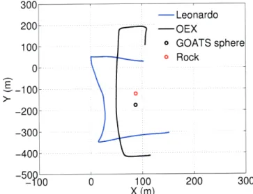
4-2 Location of the OEX and Leonardo during the run . ... 50
4-3 Experimental scattering strength of the GOATS sphere . ... 51
4-4 Ricker pulse applied to the Lubell source . ... . . . 52
4-5 Calibration setup of the Lubell source . ... . 52
4-6 Transmitting voltage response of the Lubell source measured during cali-bration . . . .. . 53
4-7 Depth of the Lubell source during the run . ... 55
4-8 Stack of pings . . . 57
4-10 Predicted time of arrivals of the multipath echoes . ... 58
4-11 Experimental time of arrivals of the multipath echoes . ... 58
4-12 Elastic target echo -First and second singular value . ... 60
4-13 Elastic target echo -Third and fourth singular value . ... 61
4-14 Rock echo -First and second singular value . ... 61
4-15 Rock echo -Third and fourth singular value . ... . . . 62
4-16 Singular Values associated with the echo from the elastic target ... 63
4-17 Free field backpropagation of the first singular vector . ... 64
4-18 Free field backpropagation of the second and third singular vector ... 64
4-19 Singular Values associated with the echo from the rock . ... 65
4-20 Free field backpropagation of the first singular vector . ... 65
Chapter 1
Introduction
1.1 Background and Motivations
Recent developments in Autonomous Underwater Vehicles (AUVs) technology have brought new perspectives in various fields of ocean engineering such as oil exploration, fishery, ma-rine archeology and mine countermeasures (MCMs). The deployment of autonomous ve-hicles requires significantly less manpower than surface vessels and is often better adapted to exploring areas with limited access. For economic reasons, the choice of inexpensive platforms to collect data also presents competitive advantages for many applications. The costs involved in mine hunting missions conducted from military ships are reduced by us-ing AUVs which also allow for safer, cooperative and inexpensive operations. However, the shift toward smaller platforms for MCMs as well as for many other fields also intro-duces new challenges, each of which calls for innovative solutions.
Power limitations onboard AUVs impose reduced power-budgets allowable for the pro-cesses running on the payload and call for efficient algorithms. The efficiency of active Detection Localization and Classification (DCL) techniques in the field of MCM can be measured in terms of coverage rates and false alarm rates. Coverage rates are typically constrained by the frequency band of the detection signals. High frequencies ('MHz) used by side-scan sonars provide high-resolution images of the seafloor at the cost of
seawa-ter. In addition, the poor bottom penetration of high frequency signals also prevents their use for the detection of mines buried in the seabed. In comparison, low-frequency signals (-kHz) suffer little transmission losses, penetrate deeper into the seabed and can reveal the structural response of mine-like elastic objects [1]. The scattering from elastic spherical shells at low-frequency has been investigated during past experiments [2] [3] along with the development of high-fidelity numerical models that can now treat a broad class of scat-tering problems [4] [5]. The sampling of low-frequency scattered fields using AUVs has long been problematic due to the lack of control techniques adapted to the towing of long receiving antennas by a small platform. A behavior-based control approach [6] recently tested at sea with a 100m long array towed behind a 21 inch AUV demonstrated robust control maneuvers and brings promising sensing capabilities for AUVs.
The presence of multipath and reverberation in shallow waveguides greatly compli-cates the detection of target echoes and constitute a limiting factor for most DCL tech-niques. Therefore, the focusing of acoustic energy on potential targets is desirable in order to achieve higher signal to noise ratio. In homogeneous and unbounded media, focusing monochromatic signals in space can be achieved with a set of acoustic sources by properly choosing their amplitude and relative phase delays. Beamforming techniques are com-monly used to estimate this weighting from geometrical approximations and produce with an array of sources, a set of pressure wave-fronts that interfere constructively in the focus-ing region. In ocean waveguides, however, the task of estimatfocus-ing appropriate amplitude and phase delays that account for boundary reflections becomes intractable without the knowledge of the environment. In contrast, the Time Reversal (TR) process automatically determines the response of the waveguide from the scattered field measurements to com-pensate for multipath effects. The ability of the TR acoustics methods to achieve focusing in time and space without prior knowledge of the environment has attracted a lot of atten-tion among acousticians [7] [8] [9] [10]. Focusing techniques based upon the TR process have been developed to handle multiple scatterers and extract simultaneously the location
1.2 Thesis objectives
The main objective of this research is to investigate the concurrent detection classification and localization of seabed objects using a TR approach. The DCL technique involves a sin-gle acoustic source and a set of receivers in a bistatic configuration. The source insonifies the target field at low frequency while the scattered field is sampled with a receiving array towed behind an AUV. The detection of the scatterers requires the analysis of invariants of the TR process determined from the singular value decomposition of the TR operator. The localization of the scatterers is then achieved with a Time Reversal imaging of the seabed, best described as a "virtual" TR mirror since it does not imply actual acoustic transmis-sions. Due to the limited amount of calculations involved in the detection and localization process, this approach is well suited to AUV operations. In order to meet our objective, we consider the following intermediary steps:
* Modeling of realistic operational scenarios to test the feasibility of the virtual TR mirror approach and understand its limitations
* Implementation of the TR imaging used to localize the seabed targets * Testing of the virtual TR mirror approach with experimental data
1.3 Thesis Outline
The thesis report will be organized as follows:
The second chapter introduces the theoretical concepts upon which the proposed ap-proach is based. In particular, the derivation of several focusing methods is presented to formulate the relations between the eigenstates of the TR process and the scatterers present. The theory on scattering from elastic spherical shells is also reviewed. The chapter con-cludes with the review of past research work in the field of Time Reversal acoustics.
The third chapter describes the modules involved in the modeling of the broadband in-sonification of a shallow water waveguide in presence of targets located on the seabed and the measurement of the resulting scattered field at the receiving array. It also provides jus-tifications for the modeling simplifications made to reduce computation time while main-taining modeling accuracy. Finally, the principle of the virtual Time Reversal mirror used localize the scatterers on the seabed is presented along with the analysis of simulated re-sults.
The fourth chapter presents the setup of the sea trial that took place near the island of Palmaria (Italy) in January 2008 and the steps taken to process our experimental data. In particular the time of arrival of echoes from the scatterers are determined from the analy-sis of the singular value of the TR operator and compared to the time of arrival estimated using geometrical consideration. The localization of the scatterers based upon the virtual time reversal mirror approach is also compared to known positions of the scatterers present. The last chapter concludes the thesis and summarizes the simulated and experimental results. In light of observations made, several limitations of the proposed approach are presented along with possible future developments.
Chapter 2
Theoretical Background
This chapter introduces the theoretical concepts underlying the virtual TR mirror approach presented in the third chapter of the thesis and reviews past research work in the field of Time Reversal Acoustics.
2.1
Time Reversal Acoustics
2.1.1 Background
The wave equation governing the propagation of pressure waves in lossless inhomogeneous media is given by:
p (r)V1 Vp 0 (2.1)
( (r) c2(r) ( t2
where p, c, and p refer respectively to the pressure, sound speed and density in the medium. Since the order of the time derivative in Eq. (2.1) is even, if a function p(r, t) satisfies the wave equation, its time reversed form, p(r, -t) is also a solution of the wave equa-tion. From a practical aspect, the invariance of the wave equation to time inversion implies that the field emitted from a source can be recorded, time reversed and focused back at the source location as if time was running backwards. Achieving time reversed focusing
requires that time shift invariance, linearity and reciprocity hold in the environment. Time Reversal mirrors (TR mirrors) are physical implementations of the time reversal procedure. The TR mirror typically consists of a set of receivers connected to a storage device that records the pressure field incident on the mirror. A set of sources co-located with the receivers of the TR mirror retransmits the recorded signals in a time reversed manner (First In Last Out). During the backpropagation, the acoustic field produced by each source of the TR mirror interferes constructively where the pressure field initially measured by the TR mirror was emitted and destructively elsewhere. TR mirrors are well suited for active detection purpose since they allow to focus energy on reflective scatterers playing the role of sources after insonification of the environment.
2.1.2 Time Reversal process
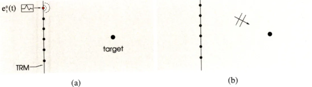
We describe in more details the steps involved in a focusing cycle in presence of a single scatterer in a free field environment. The sources of the TR mirror first insonify the envi-ronment with a set of probing signals em (t) (m = 1, ..., N assuming N sources) (Fig. 2-1).
e (t) E -:
target
TRM-(a) (b)
Figure 2-1: Target Insonification
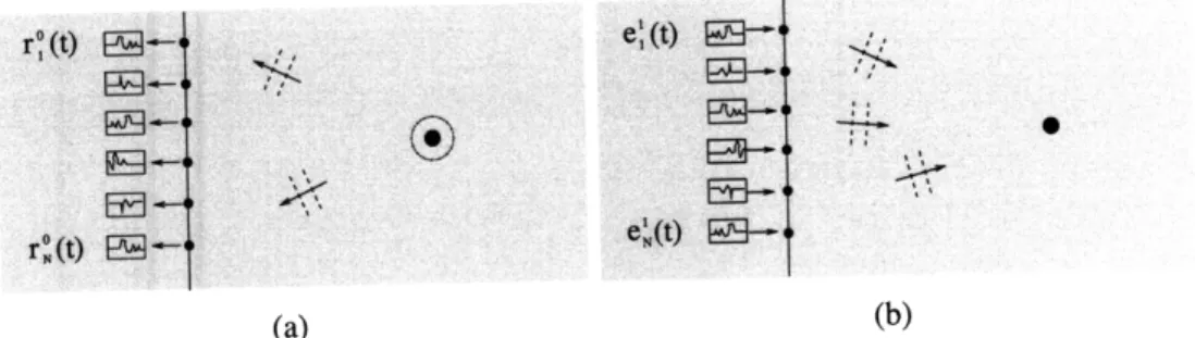
The resulting scattered field measured at the 1th receiver of the TR mirror (1 = 1, ..N)
(Fig. 2.2(a)) is expressed as follows:
N
r(t) = kim(t) 9 em(t) (2.2)
where kim(t) is the impulse response between element m and element I of the TR mirror. "0" denotes the time domain convolution. In the frequency domain, Eq. (2.2) becomes:
(2.3) Ro(w) = Kim(w)Eo(w)
m=1
where the 0 index refers to the initial cycle.
FE--A
ro(t) Pq_
C~ (t)~
Figure 2-2: Backpropagation in presence of a single scatterer
The field recorded at the receivers is then time reversed or equivalently phase conju-gated in the frequency domain. The new set of signals to be transmitted (Fig. 2.2(b)) in order to focus on the target is expressed as:
N Ell(w) = Km(w)E,*(w) m=1 (2.4) or in matrix notation: El(w) = K*(w)EO*(w) (2.5)
where K(w) refers to the interelement matrix evaluated at the frequency w.
In presence of a single scatterer, repeating the focusing cycles progressively reduces the extent of the focusing region and converges to an optimized set of amplitudes and phase delays associated with the scatterer. The analysis of convergence of successive focusing
cycles in presence of multiple scatterers yields the iterative focusing approach.
2.1.3 Iterative Focusing Approach
In presence of multiple reflectors, the procedure described in section 2.1.2 is repeated in order to focus on the most reflective scatterer by iteratively filtering the scattered field of weaker reflectors. This self-converging process initially formulated by C.Prada [12] yields without calculations the amplitudes and phase delays that are to be applied to the sources of the TR mirror in order to achieve focusing on the dominant scatterer. We proceed with an analysis of convergence of the iterative focusing approach in presence of a set of d point-like scatterers (where d < N) with distinct reflectivities.
The focusing procedure introduced in section 2.1.2 yields the signals to be transmitted
by the TR mirror in order to focus on the scatterer present. The same approach applies in
presence of multiple well-resolved' scatterers and results in a transmitted field that initially focuses on each of them. Starting from Eq. (2.5), the scattered field resulting from the transmission of E'(w) by the TR mirror is given by:
Rl(w) = K(w)El(w) (2.6)
and yields the transmitted signal of the next cycle:
E2(w) = Rl*(w) (2.7)
= [K*(w)K(w)]E(w) (2.8)
K*(w)K(w) in Eq. (2.8) is referred to as the Time Reversal operator (TR operator).
Since reciprocity holds in the environment, the interelement matrix K is symmetric and consequently the TR operator matrix is hermitian, has real positive eigenvalues and orthog-onal eigenvectors. In presence of point-like well-resolved isotropic scatterers, the rank of
1Scatterers are said to be well-resolved when the field focused on one of them does not insonify the other
the TR operator is equal to the number of reflectors present [13] and each eigenvalue Ai(w)
(i=l,...,d) (and corresponding eigenspace) is associated with one of the reflectors present.
Therefore, any vector can be expressed as a combination of d non-null vectors from these eigenspaces. For example, the first transmission vector EO(w) can be expressed as:
EO(w) = Fi(w) + F2(w) + ... + Fd(w) (2.9)
where Fi(w) is a vector from the ith eigenspace. Using this form of EO(w), the trans-mitted signals corresponding to the 2n iteration and given by:
E2n(w) = [K*(w)K(w)]Eo(w) (2.10)
can be rewritten as:
E2"(w) (W) F= ) + A (w)F2(w) + ... + )Fd() (2.11)
Similarly the transmitted signals corresponding to the 2n + 1 iteration expressed as:
E2n+(W) = [K*(w)K(w)lnK*(w)E*(w) (2.12)
can be rewritten as:
E2n+1(A) n(w)K*(w)F*(w) + ... + A (w)K*(w)F*(w) (2.13)
For a large number of iterations, Eq. (2.11) and Eq. (2.13) converge respectively as follow:
E2n () n )(w)F(w) (2.14)
where j is the index associated with the largest eigenvalue of the TR operator. Eq. 2.14 shows two distinct limits of convergence of the iterative approach both associated with the dominant scatterer. The DORT method described in the section 2.1.4 extends this analysis
to the remaining eigenvectors of the TR operator to achieve selective focusing on the each scatterer present.
2.1.4
DORT Method
The DORT2 method enables selective focusing in a multiple-scatterer environment. The technique consists of the following steps:
1. Construction of the interelement matrix K(w),
2. Extraction of the eigenvalues and eigenvectors of the TR operator (= K* (w)K(w)),
3. Focusing on a selected scatterer by transmission of its associated eigenvector. The formulation of the DORT method is a direct consequence of the convergence analy-sis of the iterative focusing approach. It was demonstrated in section 2.1.3 that the iterative approach yields the focusing on the strongest scatterer present. The following derivations show that in the presence of point-like well-resolved isotropic scatterers of different reflec-tivity, the transmission of each eigenvector of the TR operator allows for the focusing on its associated scatterer.
Considering the transmission of an impulse signal 6(t) from the location of the ith scatterer present, the field measured at the TR mirror by the 1th receiver is expressed as
ar(t) 0 hil(t) where ar(t) is the acoustoelectrical response in reception of the receivers of the TR mirror. For simplicity the receivers of the array are assumed to have identical response in reception. hit(t) referes to the diffraction impulse response between the ith
scatterer and the 1th receiver of the TR mirror. The field to be emitted by the Ith source of the
TR mirror in order to focus at the location of the ith scatterer is given by ar(-t) 0 hil(-t)
and the pressure field at the location of the jth scatterer after the time reversed transmission is expressed as:
N
Pj(w) = A*(w)Ae() Hj(1 w)H(w) (2.15)
l=1
2
The term Ae(w) in Eq. (2.15) refers to the Fourier transform of the response in emission of the sources of the TR mirror. For simplicity the sources of the array are assumed to have identical response in emission.
In a vector form Eq. (2.15) becomes:
P(w) = A (w)Ae() THj(W)H*(w) (2.16)
The condition of well-resolved scatterers implies that the vectors Hi (w) are orthogonal and that the field produced at the jth reflector and given by equation (2.16) is null unless
i = j. The preceding analysis demonstrates that propagating HZ (w) from the TR mirror
allows to focus on the ith reflector present. We now show that Hj(w) is the eigenvector
of the TR operator associated with the eigenvalue Ai (w). Transmitting HZ* (w) from the TR mirror produces a scattered field measured at the TR mirror an d given by K(w) H (w). The component of the scattered field measured at the receiver I is expressed as:
N
R, (o) = Hi* (w)K,(w) (2.17)
m=l
Introducing the reflectivity of each scatterer C, (w), Cz(),...,Cd(w), the interelement2 frequency response Kmi (w) can be related to the diffraction response as follows:
d
Km (W) = Hmkc(W)Ck()Hkl(W) (2.18)
k=1
Using the fact that the diffraction responses are orthogonal, Eq. (2.17) becomes:
N R,(w) = Hi (w)C(w)) IH m()1Him 2 (2.19) m=1 or in a vector form: N K(w)Hf (w) = C(w) IHim ()2H (W) (2.20) m=l
Finally multiplying Eq. (2.20) by K*(w) and replacing K(w)*Hi(w) by its form in Eq. (2.20) yields:
K*(w)K(w)Hj(w) = I(W) 12 Him(W) 12 Hi (w) (2.21)
(N=2
From Eq. (2.21), it is clear that the eigenvector H* (w) of the TR operator is associated with the eigenvalue AiX(w) defined as :
Ai(w) Ci(w) 2 ( Him() 2 (2.22)
Thus the magnitude of each eigenvalue is equal to the square of the effective reflectivity of the corresponding reflector. It is important at this point to make the distinction between the effective reflectivity of the scatterer and its structural reflectivity. The form of AX(w)
shows that the effective reflectivity of a scatterer depends on the coefficient of reflexion but also on the transmission between the scatterer and the receivers of the TR mirror.
The iterative focusing approach generates a vector field that converges to the eigen-vector produced by the DORT method for the dominant scatterer. However in presence of scatterers with similar effective reflectivities, the convergence process requires a large number of iterations. Furthermore, it does not provide any of the eigenvectors associated to the weaker scatterers present. In these regards, the DORT method overcomes the lim-itations of the iterative focusing approach but does so at the cost of the time consuming construction of the TR operator which is not needed by the iterative approach. The in-terelement response kl,(t) between element L and element m is measured by emitting an impulse from the source 1 of the TR mirror and recording the scattered field at the receiver
m. Due to the reciprocity of the transmission, kim (t) = kml(t) and for a TR mirror of N
element the construction of the TR operator requires N2/2 measurements. An alternative
approach well suited to reverberating waveguides has been introduced by Lingevitch [14] and results in higher signal to noise ratios during waveguide insonification. A set of beams defined by orthogonal weighting vectors at the transmitting array is used to insonify the
waveguide in place of the conventional insonification from individual sources. The process results in a "beam space" interelement response matrix from which the "element space" interelement response is recovered with a simple matrix manipulation.
2.1.5
Covariance matrix representation of the TR operator
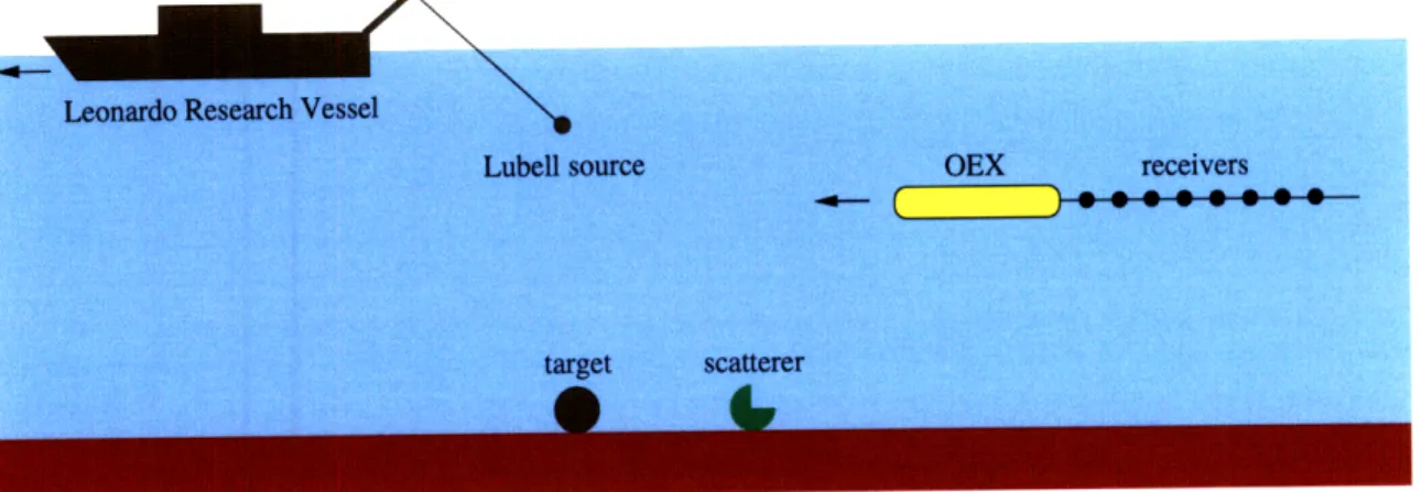
In section 2.1.3 and 2.1.4, the construction of the TR operator is formulated for a set of stationary co-located sources and receivers. The virtual TR mirror approach presented in this thesis however involves a moving source that insonifies the waveguide at regular time
intervals and a receiving array towed behind an AUV (Fig 4-1).
Lubel source OEX receivers
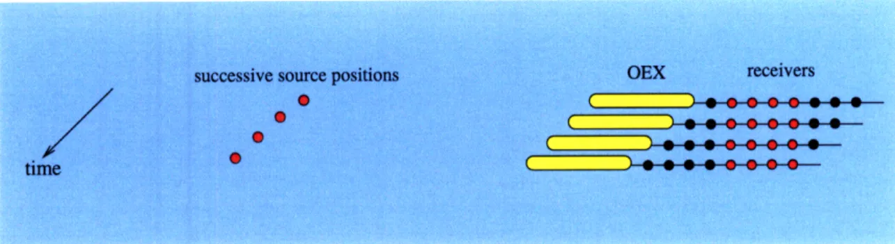
Figure 2-3: Bistatic configuration envisioned for the virtual TR mirror approach Here, the condition of a stationary array is re-created by restricting our processing to a set of receivers that overlap at the time of emissions of the source. In the configura-tion described here, Doppler shifts are introduced due to the relative moconfigura-tion between the source and the targets and due to the motion of the receivers relative to the target. However, since the waveguide is insonified at low frequency and since the speed of the source of the receivers is small Doppler effects are assumed to be negligible. Therefore the source is considered stationary at each time of emission and it re-creates from its successive posi-tions a stationary transmitting array (Fig 2-4).
Figure 2-4: Set of receivers chosen for the construction of the TR operator
For configurations that involve separated array of sources and receivers, invariants of transmissions of the TR process are identified with a similar approach as described in sec-tion 2.1.3: the interelement matrix K is constructed by measuring the field incident on a stationary receiving array subsequent to successive emissions of probing signals from each source of the transmitting array [8]. The Singular Value Decomposition of the interelement matrix (or equivalent eigenvalue decomposition of the TRO = K*KT) provides each eigenstate of the TR process. This form of the TR operator that differs from the previously introduced K*K, allows to obtain a Hermitian matrix from non-symmetric interelement matrix [15] which is particularly useful in channels where the short time coherence affects the reciprocity. Our approach to construct the TR operator (in the form K*KT) involves a passive source detection technique based on the decomposition of the covariance matrix. We present below some of the steps of the construction of the covariance matrix described in [10] [16] [17].
Assuming a linear time-invariant environment where d sources emit the signals si (),...,
Sd(t) measured by L receivers. The signal measured at receiver 1 is given by: d
rt(t) = hi(t) 0 si(t) + b(t) (2.23)
i=-i
where h1 (t) refers to the impulse response from the source i to the receiver 1. b(t) refers
to the noise signal measured at the receiver. In the frequency domain, Eq. (2.23) yields the following matrix formulation:
R(w) = H(w)S(w) + B(w)
where H(w) is the transfer matrix from the sources to the receivers and B(w) is the noise vector. Each of the M realizations is associated with the column vector R, (w) of the received signal. An estimate of the covariance matrix is obtained from :
C(w) = ZRm(w)T Rm(w)* (2.25)
m
Assuming that the background noise and the sources are mutually decorrelated, the covariance matrix is expressed as:
(C(w)) = H(
)(S(w)S(w)*)H(w)*
*+ (B(w)B(w)*) (2.26)The assumption of uncorrelated sources yields:
H(w) (S(w)'S(w)*)T H(w)* = (jS(w) 2)H(w)TH(w)* (2.27) Also assuming an incoherent background noise yields:
(B(w)TB(w)*) = 02I (2.28)
Combining Eq. (2.26), Eq. (2.29) and Eq. (2.28), the diagonalization of the covariance matrix is given by:
L
A = ( Si () 1Hei(w) 2 + 2 (2.29)
l=1
For the implementation of the virtual TR mirror approach, the TR operator is con-structed from the estimated covariance matrix given in Eq. (2.25). The sum over several source realizations allows to average out the noise contribution in the measured signals.
2.2
Scattering from elastic targets
The classification of seabed objects as "elastic target" or "clutter" relies on the compari-son of their response subsequent to an incident acoustic field. In the context of the DORT method, the singular value decomposition of the TR operator constructed from successive scattered field measurements provides classification information for each target present. However understanding the characteristics of the scattered fields associated with objects of different nature is essential to implement a reliable classification procedure based on the resulting singular values. In this section, the scattering from elastic spherical shells sub-sequent to a plane wave insonification is introduced with an emphasis on the differences between the scattering from rigid (i.e high density contrast) and elastic objects.
The Resonance Scattering Theory originally introduced in quantum mechanics and first applied to classical physics by Flax [18] has been used to investigate various acoustic scat-tering problems involving elastic objects. The formulation of scatscat-tering problems with the Resonance Scattering Theory underlines the physical meaning of each component of the scattered field and their angular dependence. The scattering from cylinders and spheres has been studied based upon this approach. We examine in this section the scattering in free field resulting from a plane wave incident on a spherical shell. A complete analysis of the scattered field from elastic spherical shells based upon the resonance scattering theory has previously been reported [19] and [20]. Here, we present several of the steps of the derivation presented in [20] along with properties of the elastic waves given in [1].
Given a plane wave insonification of amplitude po expressed as:
pi = po exp[i(kr - wt)] (2.30)
The scattered field from an elastic spherical shell takes the form:
00
s = po exp[-iwt] E i(2n + 1)Rh() (kr)P(cos(O)) (2.31)
where R, is a function of the wavenumber k of the incident plane wave and a the outer radius of the spherical shell which involves the density and phase speed of the shell material and surrounding medium. r is the radial distance from the center of the shell,
n is the modal order, h(1) is the spherical Hankel function of the nth order and P, is the
Legendre polynomial of the nth order. The partial-wave scattering function S, and the scattering phase shift 6, are related as follows:
Sn = 2R, + 1 - exp(2i3n) (2.32)
Introducing the form function f (0) expressed as a sum of partial waves functions
00
f(0) = E f (0) (2.33)
n=O
f,(0) = (2n + 1)S /2 sin 6,P,(cos(0)) (2.34) and the asymptotic representation of the spherical Hankel function
h() (kr) i - (n+l) exp(ikr) (2.35)
n kr
The scattered field in the limit r > oc takes the form
Ps Po exp[i(kr - wt)]f(0) (2.36)
2r
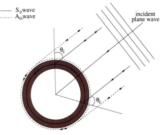
The scattering from elastic objects can be represented as the superposition of a rigid body contribution and a radiation contribution. For thin spherical void elastic shells, the radiation contribution at frequency (i.e for small values of ka) is limited to the low-est order compressional and flexural modes and their respective circumferential Lamb-type waves: the symmetric wave So and antisymmetric wave A0. Upon fluid loading, the
an-tisymmetric wave A0 bifurcates into two dispersive waves A0- and Ao+. The symmetric
So wave is supersonic and reradiates periodically out of the spherical shell at the coupling
Oc = arcsin ( t) (2.37)
( Cshell )
where cxt refers to the sound speed of the surrounding medium and Cshel refers to the phase speed of the So wave in the shell. Fig. 2-5 depicts the travel paths of the Ao- and So Lamb-type elastic waves backscattered by a spherical shell after insonification around the
coincidence frequency. The radiation angles are outlined for the two wave types.
At higher frequencies, the amplitude of the response of the elastic target increases within the mid-frequency enhancement region where the phase speed of the Ao- wave approaches that of the surrounding medium and reaches a maximum at the coincidence frequency fc defined as:
Cext
fc
2xdird (2.38)where d defines the shell thickness. From the measurement of the time of arrival of the So reradiated waves, Eq. (2.38) can be used to estimate the shell thickness. As the frequency increases above the mid-frequency enhancement region the number of modes excited increases.
S owave
SAowave incident
The dissipation of the circumferential waves determines the number of reradiation de-tectable and consequently the duration of the elastic response. The scattering from rigid objects defined by large density contrast with the surrounding medium, differs from that of elastic objects in that the radiation contribution is negligible and the scattered field reduces to the specular echo of the incident field. From the perspective of the TR operator, the presence of the elastic response in the scattered field introduces new invariants of transmis-sion and therefore additional eigenstates of the TR process associated with the modes of the target. As a result, for similar configuration and target size, the number of significant singular values associated with an elastic target is expected to be larger. In a waveguide, the number of singular values associated with an object also depends on the presence of boundaries that introduce its images and therefore virtually extends its size.
2.3 Literature review
2.3.1 Iterative Focusing Approach
In 1989, Fink extended the phase conjugation method -used in optics to correct the wave-front distortion affecting monochromatic signals -to broadband signals with the formula-tion of the Time Reversal Mirror [21]. The time reversal process was first applied to the problem of focusing through aberrating media in pulse echo mode and to selective focusing in presence of multiple scatterers. Numerical simulations of the iterative focusing approach were presented in 1991 [22] to examine the effect of the array aperture and of the differ-ence of reflectivities between scatterers. In 1995, the convergdiffer-ence of the iterative focusing method was investigated for well and poorly resolved scatterers [12]. The theoretical anal-ysis showed distinct limits of convergence for odd and even number of iterations. The number of iterations needed to achieve convergence on the dominant scatterer was found to depend on the differences of reflectivity between the scatterers. The iterative focusing approach was explored at sea in 1999 [23] with a TR mirror spanning the water column and a receiving array located at the focusing range. A probe source was used in place of a scatterer to insure higher signal to noise ratios and the field transmitted by the TR mirror
after each iteration was amplified. A spread in time of the signal measured at the retrofocus location was attributed to the bandpass filtering introduced by the transducers of the TR mirror and the waveguide. In 2004, Montaldo [24] proposed a solution to the problem of time spreading. The method based on the iterative focusing approach resolves the wave-fronts associated with each scatterers from the signals measured at the TR mirror. Each set of wavefronts detected is then recompressed in time prior to its retransmission to limit the bandpass filtering introduced by the transducers of the TR mirror and the waveguide. The same authors [25] introduced a new method based on the iterative focusing approach that involves two Source Receivers Arrays (SRA). A control array measures the field produced by the emitting array and compares it to a objective/desired field at the control array. The difference between the desired field and the measured field at the control array is then used to adjust iteratively the field transmitted from the emitting array and successively achieve optimum focusing. This technique overcomes the time spreading effects mentioned earlier and allows to achieve optimum focusing faster and with little computation efforts.
2.3.2
DORT method
In order to provide the reader with an organized literature review of the DORT method, the following section is divided into categories of problems to which the DORT method has been applied. Within each category, the publications are presented in chronological order.
Selective focusing on point-like and extended scatterers
In 1993, the theoretical formulation of the DORT method was introduced from the
deriva-tion of the iterative focusing approach [26] and the predicderiva-tions made with the method were confirmed by simulated results [11]. The selective focusing based on the DORT method was investigated theoretically for well-resolved wires and the focusing ability of the DORT method was compared to that of the iterative approach for the most reflective scatterer of a set. Experimental results showed that both methods have the same ability to focus in space however the DORT method achieves focusing with only one iteration. Prada extended the DORT method to a finite size hollow cylinder and found that each eigenstate of the TR
operator is associated with a circumferential elastic wave and two points of emission on the cylinder [27]. The experimental backpropagation of each eigenvector confirmed this analysis and allowed an accurate estimation of the phase speed associated with each type of wave. In 1996, the special case of selective focusing on two targets with same apparent reflectivities was investigated theoretically and experimentally [7]. In such configuration, the DORT method produces two eigenvectors with unique characteristics. The magnitude of the first eigenvector shows in-phase contributions of the two targets while the second eigenvector shows their out-of-phase contributions. Selective focusing in this case requires the backpropagation of a linear combination of the two eigenvectors. In light of these re-sults, the scattering analysis from the hollow cylinder conducted in 1994 was revisited [28]. The two secondary sources (associated with the radiation of elastic waves) have identical "reflectivities" and as observed for the two well resolved wires, the DORT method results in two eigenvectors whose magnitude exhibit interferences of these secondary sources radiat-ing in-phase and out-of-phase. In 2001, Chambers carried out the theoretical analysis of the time reversal process associated with a homogeneous point-like scatterers (i.e. subwave-length and spherical) and demonstrated that one eigenstate of the TR operator is associated with the compressibility contrast between the scatterer and the medium while three other eigenstates are associated with the density contrast [13]. The analysis of the TR opera-tor conducted on subwavelength isotropic and anisotropic cylinders results in observations validated by ultrasonic experiments [29]. Chambers applied the theoretical analysis of the DORT method to finite objects of simple geometry such as spheres and finite objects of arbitrary geometry in far-field configurations and confirmed theoretically the relation be-tween the number of eigenvalues associated with an extended scatterer and its size [30]. Minonzio investigated the relation between the modes of vibrations of an elastic scatterers (caused by the density and compressibility contrasts), the projected harmonics associated with each mode and the singular values of the TR operator [31]. In particular, the maxi-mum number of projected harmonics resolvable by the receiving array yields the possible reduction of the dimension of the TR operator.
Environment effects on selective focusing
In 1995, the selective focusing method was tested with a layer of inhomogeneous aberrating media separating the TR mirror from the scatterers [32]. It was shown experimentally that selective focusing on well-resolved scatterers can be achieved under the condition that the phase variations introduced by the layer of aberrating medium are smooth. In 1999, Mor-dant showed significant improvements in resolution obtained when focusing in a waveg-uide. Each image of the TR mirror relative to the waveguide boundaries virtually increases its extent and allows for higher resolution focusing compared to predicted resolution in free field. The effects of time variance of the environment on the selective focusing were investigated experimentally in presence of waves of varying amplitude [9]. It was observed that increasing the wave amplitudes increases the amplitude of the noise eigenvalues and decreases the amplitude of the eigenvalues associated with the targets. Finally, Mordant formulated the condition for selective focusing in time and space. The time domain DORT method requires that the reflectivity of each scatterers present in the waveguide allows to attribute to each of them the corresponding eigenvector over the frequency band of a short duration pulse. A similar study from Roux [33] also provided an analysis of the tempo-ral focusing in the waveguide and genetempo-ral formulations for the size of the focal spot and sidelobe levels around the focal spot. In particular, it was observed that the size of the retrofocus increases when the insonifying source is located near the interface. Sabra and Dowling reported on the effect of background noise [34], array motion [35], array de-formation [36] and ocean currents [37] on retrofocusing in shallow water environments providing theoretical background for realistic time reversal scenarios in ocean waveguides. The effect of bottom absorption and reverberation on the resolution of the focusing have been investigated [38] and a method was presented to compensate for transmission losses affecting each multipath between the TR mirror and the scatterer and improve signal to noise ratio at the scatterer but requires prior knowledge of the environment. In the light of earlier investigations showing degraded retrofocus in reverberating environments, several solution were proposed that attempt to reduce the amount of backpropagated field reaching the seabed at the focusing range. Kim [39] discussed the potential benefits of using a
prob-ing source located at mid-depth to determine the field to be transmitted by the TR mirror in order to produce a null of transmission near the bottom at the range of the probing source. A similar approach consisted in insonifying a mid-depth target with a probing source and showed improvements in the backpropagated field reaching the target. The use of a prob-ing source however limited the potential of these approaches. Instead, simulated results from Song [40] explored the possibility of determining the eigenvector associated with the seabed reverberation at a range of desired focusing to generate a nulling vector by linearly combining the remaining orthogonal eigenvectors of the TRO. [41]
Time Reversal Imaging
The localization and shape estimation of extended targets based on TR imaging has been in-vestigated in publications related to inverse problems. In 2004, Hou layed out an approach based upon the coupling of the target location estimation with a shape estimation algorithm based upon a level set method [42]. In 2007, Hou examined the construction of imaging functions for several types of scatterer boundary conditions (i.e. scatterer properties) [43] which were used to determine the location of the target and its boundaries using a prior es-timation of the number of singular values associated with the target subspace. The number of target associated eigenstates was determined by comparing ratios of singular values to a predetermined threshold. It was observed during numerical experiments that the resolution of the focusing is found to improve when estimated boundary conditions considered for the imaging functions match actual boundary conditions at the scatterer. Carin [44] presented similar observations in presence of a strong scatterer, the waveguide characteristics which are unknown and supposed for the TR imaging of the scattered field can be adjusted until an optimum focusing is reached.
Chapter 3
Modeling of the virtual TR mirror
approach
3.1
Introduction
In order to predict the performance of the concurrent detection classification and localiza-tion method based on Time Reversal, a numerical model of the virtual TR mirror approach is implemented. The model allows the localization of the seabed targets by transmitting the singular vectors of the TR operator (see Chapter 2) and also provides valuable insights into the method's limitations,. Since the backpropagation does do not involve actual transmis-sions underwater, the process is referred to as a "virtual Time Reversal mirror". In order to meet the limited power constraints imposed by autonomous operations, the amount of computations involved is minimized by making appropriate simplifications on the model-ing. The steps taken to simulate the target insonification, target scattering, and scattered field measurements are described in the first section of this chapter with an emphasis on the underlying theory. The second section explains the implementation of the virtual TR mirror, presents results and summarizes observations made from the simulations.
3.2 Scattered field modeling
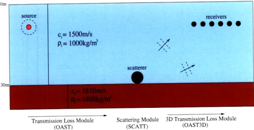
An overview of the modules involved in the modeling of the virtual TR mirror approach is shown on Fig. 3-1.
Transmission Loss Module Scattering Module 3D Transmission Loss Module
(OAST) (SCATT) (OAST3D)
Figure 3-1: Overview of the modeling steps
3.2.1
Target insonification
-
OAST
The waveguide characteristics considered in this section are chosen to reflect the sea trial during which the virtual TR mirror approach was tested. The sea trial was conducted during the winter of 2008 in a shallow waveguide (30m deep). For modeling purposes, we assume an isospeed water column of 1500m/s. In absence of bottom properties measurements, we make the assumption of an isospeed bottom and use table values corresponding to a sandy bottom [45]. Considering the previous assumptions and the fact that the bathymetry in the area of the sea trial is roughly constant, the propagation environment is conveniently mod-eled as a Pekeris waveguide.
In a range independent waveguide, the Helmholtz equation satisfied by the total field in each layer takes the following form':
[V2 + k2(z)<(r) = f(r) (3.1)
where k is the wavenumber, b the field parameter of interest and r is the position vector
A common approach to solving the Helmholtz equation (3.1) is the use of integral trans-forms: the total field is decomposed into plane waves defined by their individual horizontal wavenumbers. This approach simplifies the treatment of the boundary conditions at each layer interface of the waveguide. The Hankel transform pairs are given by:
f (r, z) = f (kr, Z) Jo(krr)dk, (3.2)
f (kr, z) =
f
(r, z)Jo(krr)dr (3.3) The Hankel transform applied to the Helmholtz equation reduces the three dimensional Helmholtz equation 3.1 to the following depth-separated wave equation :+ (k2 - k) (k, z) = S 6(- (3.4)
dz2 2r12
where S, is the source strength at the frequency w, kr is the wavenumber in the radial direction, and z, is the depth of the source.
The solution of the depth-separated wave equation is obtained using the Direct Global Matrix (DGM) approach. The field within each layer of the waveguide is represented in terms of source contributions and unknown scalar fields amplitudes of up and down going conical waves [46] [47] [5]. The unknown scalar fields which are superposed to the fields resulting from the source contributions are integrated into local sets of equations which are then mapped into a global set of equations solved simultaneously for the amplitude of the
unknown scalar fields within all the layers. The implementation of this method involves some complexity but this approach is unconditionally stable.
Once the depth-separated wave equation has been solved, the field parameters of inter-est are determined in the waveguide at any given range and depth by evaluating the inverse Hankel transform (Eq. 3.2) using the Fast Fourier approximation. For practical purposes, the integration domain of Eq. 3.2 is truncated to the largest wavenumber providing signifi-cant kernel contribution. The reader can refer to [45] for the detailed derivations.
The waveguide insonification from an omnidirectional source is modeled with OAST, the transmission loss module of the OASES package (Ocean Acoustics and Seismic Ex-ploration Synthesis) developed by H.Schmidt [48]. OASES is a propagation model based on wavenumber integration and the Direct Global Matrix approach. It supports a large variety of environmental models including isovelocity fluids, fluids with speed gradient, isotropic elastic media. The transmission loss module takes as inputs the depth of the source and the characteristics of each homogeneous layer constituting the waveguide (depth of the layer boundaries, fluid density, compressional/shear sound speeds, attenuation coef-ficients). Since we are concerned with the modeling of a Pekeris waveguide, only three layers are necessary: the upper half space, the water column layer, the sea bottom layer. Solutions are provided in the frequency domain and time domain analysis is obtained by Fourier synthesis. In order to compute the field in the vicinity of a scatterer, OAST ac-cepts as an input the range from the source to the scatterer and the layer where the target is located.
3.2.2
Scattered field
-
SCATT
The scattering module of OASES called SCATT uses the incident field computed in the vicinity of the scatterer to determine the resulting scattered field using the virtual sources approach. The virtual sources approach consists in replacing the scatterer by a set of sources distributed within its volume. The strength of each source is determined so that
the field produced by the virtual sources when superimposed to the incident field, satisfies the boundary conditions imposed by the type of scatterer. In the case of elastic targets, the dynamic stiffness matrix relates the pressure on the surface of the scatterer to the normal displacement of its surface. We follow several of the step of [3] to describe the computation of the virtual source strengths.
The total pressure p and total displacement u on the surface of the scatterer are first expressed as:
P = Pi +Ps U = Ui + us (3.5) where pi and ui refer to the incident field contribution. ps and us refer to the scattered field contribution.
Considering a set of N virtual sources of strengths s, the scattered field contribution is expressed as:
Ps = Ps us = Us (3.6)
where P and U are N x N matrices containing the pressure and normal displacement Green functions.
The total pressure is then related to the total displacement through the dynamic stiffness matrix K as follows:
p = Ku (3.7)
It is important to note that the stiffness matrix of the target is computed independently of the medium that surrounds it and can be used to treat scattering problems for different burial depth and target orientation. The stiffness matrix can be computed with an exact spherical harmonics representation in the case of spherical shells or with a finite element method for objects of arbitrary shapes. Combining Eq. 3.5, 3.6 and 3.7, the source strengths are computed using the following equation:
s = [P - KU]- 1[Kui - pi]
The scattering module of OASES, SCATT, is used to compute the virtual source strengths associated with various scatterer geometries and properties. In the special case of spherical targets, the command sphcvs3d takes the characteristics of the scatterer as an input to compute the virtual source strengths and the scattered field in the surrounding medium can be obtained from the spectral Green functions.
3.2.3 Transmission of the scattered field to the receiving array
Given the distribution of virtual sources and their respective strength, the Green func-tions from the virtual sources to the surrounding medium are computed with the command OAST3D. Since the virtual sources are distributed in a volume generally much smaller than the region of interest, the scattered field is conveniently derived in a cylindrical coordinate system [49]. Within each layer of the stratified surrounding medium, the scattered field is expressed as the superposition of the field produced by the virtual sources present (if any) and the unknown field required to satisfy the boundary conditions at the layers interfaces. It is governed by the homogeneous wave equation. In a horizontal fluid layer, the resulting displacement potential is expressed with an azimuthal Fourier series as follows:
00 cos mO
0(r, 0, z) = ~- (r, z) +
0'\(r,
z)] (3.9)m=0 sin mO
where 0'(r, z) is the contribution from the virtual sources and 0'(r, z) the contribution that satisfies the layers boundary conditions. Each contribution can be expressed in terms of horizontal wavenumber integrals as follows:
cos m0
sin mj rr) j
(3.10) (3.8)
H'4(r,0,z) j [A+kr)ekzz + AMi(kr)e-J kzZ]kJ(k~r)dkr (3.11) where kr and kz are respectively the horizontal and vertical wavenumber, sj is the jth virtual source strength to be determined and A+ and A- are the azimuthal Fourier coeffi-cients of the up and down-going planes waves satisfying the boundary conditions in each layer. The factor ,m equals 1 for m = 0 and 2 otherwise.
For the case where both virtual sources and receivers are located in the water column, the Green function becomes:
G(rrr)
41rrIrjj -=0 sin mOi sin mOj
(3.12) x<m (o
FJ[m(krr)Rll(kr)e
i zk-47r JO jmr~1,
x kr Jm(krri)dkr
3.3 Modeling implementation
The commands involved in the modeling described in sections 3.2.1, 3.2.2 and 3.2.3 are executed from a Matlab code. The position of the source and receivers are expressed in a Cartesian coordinate system centered on the elastic target. Using this representation, the computation of distances between the elements of the setup reduces to simple vector calcu-lus operations. This coordinate system also simplifies the grid points representation of the seabed described in the next section. The simulations involve a set of stationary receivers and a set of stationary sources all located at the same depth. The target modeled here is the GOATS sphere and we consider for the clutter a rigid spherical shell of dimensions identi-cal to the GOATS sphere. Each insonification from one of the source location yields a set of complex pressures at the receivers which are stored to construct the interelement matrix. For each of the frequencies of the insonifying signal, the interelement matrix is determined in order to produce the singular values and singular vectors associated with each scatterer over the frequency band of the insonifying signal.
3.4 Virtual Time Reversal Mirror
The previous section of this chapter describes the steps taken to model the waveguide in-sonification and the scattering from targets present in the waveguide. The complex pres-sures at the receivers obtained from this numerical model or from actual measurements are used to virtually transmit the time reversed scattered field from the receivers to the seabed and localize the scatterers present.
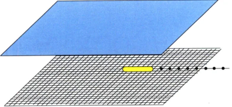
In the modeling framework introduced above, the seabed is represented as a grid (Fig. 3-2) that extends over the operating area of the AUV. The pressure amplitudes resulting from each backpropagations on the seabed are computed at every point of the grid. The Green functions required to calculate the pressure field on the seabed from the complex pressure at the receivers are precomputed using the oasp command for predefined source depths, frequencies and waveguide characteristics. At run time, the real and imaginary part of the Green functions are interpolated at the radial distances of each grid point. Since the waveg-uide is assumed to be range independent and the receiving array assumed to be horizontal, the same set of Green functions is used to compute the field produced on the seabed by all elements of the array. The resolution of the grid can be adjusted to reduce the time of computation or improve the resolution.
The backpropagation of the singular vectors can also be computed in free field as it will be discussed in the next chapter. The pressure at each grid point of the seabed is then determined by the cross product of the singular vector with the propagation vector M defined by :
M -jklr-rl -jkr-r2
e-jk
r-rn(3.13)
r -r I' Ir -r 2 r-rn
where r refers to the position vector of the grid point and rj refers to the position vector
Figure 3-2: Grid representation of the seabed
3.5
Results and observations
The modeling described in sections 3.2 and 3.4 is used to test the ability of our TR based approach to reject clutter and localize seabed scatterers in configurations similar to the set up of the sea trial presented in chapter 4. For the following, we consider a set of stationary sources and a set of stationary receivers located at the same depth in a shallow water waveguide. The targets to be detected and localized are an elastic spherical shell and a rigid spherical shell. Multiple scattering effects between targets are neglected.
3.5.1
Clutter rejection
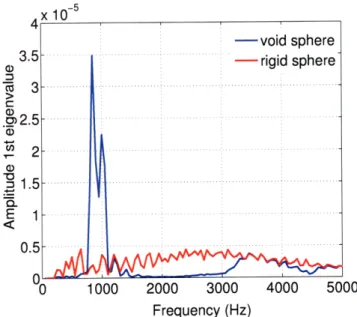
It was discussed in the second chapter that the response of elastic targets exhibits reso-nances which are not present in the response of rigid objects. In order to illustrate this point, the TR operator is constructed using the modeling of our approach in presence of an elastic spherical shell and in presence of a rigid spherical shell of identical dimensions. Fig. 3-3 depicts the amplitude of the first singular values for both targets as a function of frequency. The singular value associated with the elastic sphere clearly exhibits a resonance near 900Hz. In contrast the singular value associated with the rigid sphere does not show significant variations over the same frequency band. For elastic targets, the time of arrival of the Lamb-type waves re-radiated in the direction of the receivers varies depending on the array position and orientation. Therefore, the interference of these waves results at the receivers in time signals that differ significantly depending on the configuration source tar-get receivers. As a consequence, the frequencies at which the singular values have maxima
can not directly be used to classify the target; instead the variability of a singular value with respect to frequency can be used to classify a target as rigid or elastic.
x 10-5 -void sphere 3.5.. - rigid sphere 1.5 0 1000 2000 3000 4000 5000 Frequency (Hz)
Figure 3-3: Amplitude of the first singular value as a function of sphere and a rigid sphere
frequency for a void elastic
It is also important to observe from Fig. 3-3 that the dominant singular value is not necessarily associated with the same scatterer throughout the whole frequency band. The backpropagation of the first singular vector therefore results in a field that focuses on the
3.5.2
Selective focusing
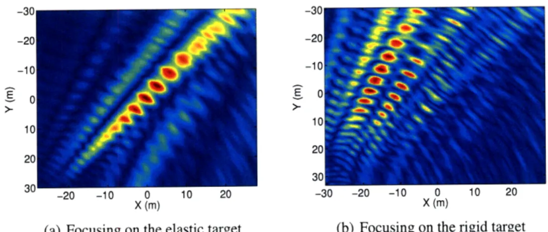
We investigate in this section the ability of the virtual TR mirror approach to localize tar-gets on the seabed. The scattered field computed at the receivers in presence of an elastic target and a rigid target is used to construct the TR operator. The backpropagation of the eigenvectors associated with each targets is achieved using the virtual Time Reversal mirror approach described in section 3.4. The receiving array considered here is composed of 20 elements spaced every 0.75m for a total length of 14.25m. In presence of well resolved scatterers (i.e scatterers separated by a distance larger than the resolution cell), the singular vectors of the TR operator provide the phase and amplitude information to focus selectively on each scatterer present. Fig. 3.4(a) and 3.4(b) show respectively the field backpropagated on the seabed for the transmission of the singular vector associated with the elastic target located at (0,0) and the singular vector associated with the rigid target located at (-20,0). We observe that the transmission of each singular vector shows a maximum at the location of each corresponding scatterer. The size of the retrofocus is related to the resolution of the array. For the smaller array extent considered during the sea trial, we expect a decrease in resolution. -30 -30 -20 -20 -10 -10 E 0 E 0 10 10 20 20 30 30 -20 -10 0 10 20 -30 -20 -10 0 10 20 X (m) X (m)
(a) Focusing on the elastic target (b) Focusing on the rigid target
Figure 3-4: Backpropagation of singular vectors associated with an elastic sphere located at (0,0) and a rigid sphere located at (-20,0) compensated for spherical spreading