APPROXIMATE INTEGRATION METHODS
APPLIED TO WAVE PROPAGATION
by
V.
WADSWORTH
DEPARTMENT
MASSACHUSET'
CAMBRIDGE
OF GEOLOGY
TS
INSTITUTE
39,
AND GEOPHYSICS
OF TECHNOLOGY
MASSACHUSETTS
U.S.
A
JANUARY, 1958
DONALD
INTEGRATION
APPLIED
TO
WAVE
PROPAGATION
by
Donald van Zelm Wadsworth
B. A., Williams College (1953)
Submitted in partial fulfillment of the requirements for the
degree of doctor of philosophy at the Massachusetts Institute
of Technology, February, 1958.
Signature of author
Department of Geology and Geophysics
Certified by
Thesis Supervisor
..001
'-k
/7
Accepted by
Chairman, Departmental Committee
on Graduate Students
ABSTRACT
APPROXIMATE INTEGRATION METHODS APPLIED TO WAVE PROPAGATION
by
Donald van Zelm Wadsworth
Submitted to the Department of Geology and Geophysics on January 27 1958 in partial fulfillment of the requirements for the degree of Doctor of Philosophy.
The standard techniques for handling the integral solutions to geophysical wave propagation problems yield results of limited applicability. Furthermore in attacking a particular problem it is not always clear which techniques should be tried, as the
relation-ships between many of these techniques are not well systematized. The purpose of this thesis is to explore new techniques based on topological considerations as well as to extend standard techniques. Also attention is given to clarifying the interrelation between the standard techniques and to relating these to the new techniques.
The principal new technique developed is the "cliff" method of integration originated by Dr. M. V. Cerrillo of the Massachusetts
Institute of Technology. This method will often yield compact solutions to integrals associated with branch cuts when well-known methods such as quadrature formulas are impractical to apply. The basic idea of the cliff method is the use of rational function approximants to replace branch cuts by chains of poles. Contour integration around the original branch cuts then can be collapsed onto the poles and the solution
obtained by the Residue Theorem.
This cliff method is generalized in two ways. First, in the
"extended" cliff method the convergence of the cliff method is improved by letting the number of poles in the approximants become infinite. For certain applications the solutions can be given in compact form. Second, the basic ideas of the cliff method are generalized by expanding the argument of a function in rational functions. The branch cuts are then replaced by more complicated singularities than the poles of the (simple) cliff method.
Finally a means is given for extending the standard saddle point methods by combining the topographic features of the saddle point methods with either the cliff methods or with quadrature methods. The solutions
are convergent and reasonably compact.
As is shown by a number of examples, the cliff methods together with the extension of the saddle point method offer a practical means
for overcoming the following limitations of standard integration methods: (1) they make it possible to extend saddle point methods to integrands having broad saddles and sharply curved steepest descent paths, (2) the cliff methods offer a simple means of handling many integrals for which quadrature methods are difficult to develop, (3) the cliff methods can handle many singular integral equations which do not readily yield to standard techniques such as Gaussian quadrature.
Thesis Supervisor: Dr. M. V. Cerrillo Research Associate Research Laboratory of Electronics
TABLE OF CONTENTS
ABSTRACT 2
LIST OF FIGURES AND TABLES 6
ACKNOWLEDGEMENT 7
BIOGRAPHY 9
INTRODUCTION 10
THESIS ORGANIZATION 16
CHAPTER I CLIFF METHODS AND BRANCH CUTS 17
Representation by Rational Functions 18
Cliff Method 24
Extended Cliff Method 27
Error Analysis 32
General Cliff Method 35
Summary 41
CHAPTER II CLIFF METHODS AND SADDLE POINTS 42
Cliff Method--Separated Integrand 42
Cliff Method--Mixed Integrand 45
Example of Cliff Method 48
General Cliff Method 49
Summary 49
CHAPTER III SADDLE POINT METHODS 50
First Order Method 52
Extended Saddle Point Methods 56
Limitations, Steepest Descent Paths 57
Quadrature Saddle Point Method 67
Summary 72
CHAPTER IV APPLICATION TO THE SOMMERFELD PROBLEM 74
Introduction 74
Formal Solution 76
Riemann Surface 77
Location of Pole 78
Approximate Methods of Solution 81
CONCLUSIONS 88
SUGGESTIONS FOR FUTURE WORK 89
APPENDIX A HANKEL FUNCTIONS 91
APPENDIX C APPENDIX D APPENDIX E APPENDIX F APPENDIX G BIBLIOGRAPHY BASIC THEOREMS RIEMANN SURFACES
Double Valued Functions Integral Transformations EXAMPLES
Cliff Method
Extended Cliff Method General Cliff Method
Cliff Method and Integral Equations GENERAL CLIFF METHOD
Contribution of Branch Cuts
Integration Around Essential Singularities with Branch Points
INTEGRATION ON BANKS OF BRANCH CUTS
97 97 99 102 102 106 106 108 111 111 112 116 126
LIST OF FIGURES AND TABLES FIGURES 0-0, 1-1, 1-5 1-6, 0-1 1-2, 1-3, 1-4 1-7 2-1, 2-2, 2-5, 2-6 3-1, 3-2, 3-4, 3-9 3-5 3-6 3-7, 2-3, 2-4 3-3 3-8 4-1, 4-2, 4-3 4-4 4-5 A-1, D-1, D-3, D-5, E-1, E-3 A-2, D-2 D-4 D-6 E-2, B-1, B-2, B-3 F-i, F-2 G-i, G-2, G-3, G-4, G-5 TABLES Page 119 120 121 122 123 124 125 124a
7
ACKNOWLEDGEMENT
I am indebted to my thesis supervisor, Dr.
M.
V. Cerrillo of the
Research Laboratory of Electronics, Massachusetts Institute of
Technology, for suggesting the thesis topic and many of the ideas on
which it is based. His guidance during many consultations was an
inspiration and invaluable in carrying out the various ramifications
of the research.
Professor S. M. Simpson and Mr. T. R. Madden of the Department of
Geology and Geophysics spent much time both in reviewing the
prelim-inary stages of the research as well as in studying the final forms
of the thesis manuscript. A number of their suggestions have been
incorporated.
Others to whom I am grateful for consultations on various aspects
of the thesis investigation include Professor L. V. Ahlfors of the
Department of Mathematics, Harvard University; Professor F. B. Hildebrand
of the Department of Mathematics, M.I.T.; Professor K. U. Ingard of the
Department of Physics, M.I.T.; Dr. J. C. Savage of the Department of
Geology and Geophysics, M.I.T.; Dr. S. C. Wang of the Lincoln
Laboratories of M.I.T.
I also wish to express my appreciation for the cooperation of
various members of the Department of Geology and Geophysics and to
the Research Laboratory of Electronics for the use of some of its
facilities.
8
Mining Co. Much of this research was carried out while I was a National
Science Foundation Terminal Fellow.
Mrs. Lena Fried of the Joint Computational Group of M.I.T. carried out most of the numerical computations. Mrs. Joan Grine made it
BIOGRAPHY
The author, Donald van Zelm Wadsworth, was born in Mamaroneck,
New York on July 14, 1931. After attending grammar schools in New
York and Connecticut, his family moved to Miami, Florida where he
graduated from Ponce de Leon High School in 1949. From then until
1953 he majored in physics at Williams College, Williamstown,
Massachusetts where he received a B. A. degree in June, 1953. The
title of his thesis was "Survey of the Most Recent Developments in
Experimental Physics". From June, 1953 until February, 1958 he was a
candidate for a Ph. D. degree in the Department of Geology and
Geophysics at M.I.T.
During high school he received an honorable mention in the
Westinghouse Science Talent Search for a paper on "Rocket Satellites
of the Earth". At Williams College and for three years of graduate
study, he was a Tyng Scholar. During his fourth year at M.I.T. he was
a National Science Foundation Terminal Fellow and was also awarded a
Postdoctoral NSF Fellowship. He is a member of Phi Beta Kappa, Sigma
Xi, the American Geophysical Union, the Society of Exploration
INTRODUCTION
Most of the geophysical problems connected with electromagnetic
and seismic wave propagation can only be solved approximately. The
method of approximate solution will depend on whether the problem is
formulated in terms of differential equations, integral equations or a
combination of these. In a particular case, it
may be easier to deal
directly with the differential equation rather than a solution in
inte-gral form. Various techniques of approximate solution such as
pertur-bation calculations, variational methods and relaxation methods are
described, for instance, by P. M. Morse and H. Feshbach in "Methods
of Theoretical Physics" and by F. B. Hildebrand in "Methods of Applied
Mathematics". Some of these methods apply especially well to scattering
and diffraction problems. However, in this thesis, we shall restrict
ourselves to approximate methods which deal with solutions already in
integral form--perhaps multiple integrals, but no unknowns in the
integrands. Nevertheless an unanticipated fruit of the research is
that one of the methods developed--the "cliff" method--has important
applications to integral equations, as described in Appendix E.
The various techniques for handling the integrals we are concerned
with can be grouped under the two classifications:
(1)
Topological Methods. These include the methods of complex
analysis which are concerned with: the nature and location of
-U I
one Riemann surface to another; the topography of a surface,
partic-ularly with respect to saddle points and steepest descent paths.
Spe-cific examples are the powerful saddle point methods of integration and
the Residue Theorems.
(2) Non-topological Methods.
These are the methods which are not
primarily concerned with the behavior
of an integrand on a surface. In
fact the variable of integration is not generalized to a two-dimensial
or complex variable. In the case of single integrals, the operations
are in one dimension only. Specific examples include the quadrature
methods of integration such as Gaussian quadrature and Simpson's rule,
expansions in orthogonal functions with term by term integration
(Fourier series, Bessel series, orthogonal polynomial series, etc.),
power series developments with summation by continued fractions and
many others.
The topological methods possess an inherent power which the other
methods lack. All the effort in the latter is concentrated on one
fixed line in the complex. In the topological methods, we consider
the whole scope of the complex plane and can see where to move our line
of integration to the best advantage. For instance, the convergence of
the non-topological methods may be very poor on part of the fixed line
because of the nearness of a singularity. In the topological methods,
we can often deform our line of integration to a less sensitive position
where the convergence is improved.
Many of the integrals appearing in the solutions to geophysical
topolog-12
ical methods of complex analysis. In general they can be put in the form
where f(z) and w(z) may be multivalued functions and may contain
param-eters. The exponential behavior of the integrand is concentrated in w(z).
L is a prescribed contour in the complex z plane. The two principal
techniques for handling these integrals are the deformation of
integra-tion contours onto steepest descent paths (which usually pass through
saddle points) or onto the singularities of the integrand. In
the former
case, the solutions are obtained by the saddle point methods of
integra-tion, while in the latter case, the solutions are obtained by the Residue
Theorem, if the singularities are poles. Of course a given problem may
require
the
use of both techniques.
For the type of integral of interest in wave propagation in
disper-sive media, these techniques have serious limitations. The saddle point
methods are asymptotic, so that the solutions are valid only in a
restricted region--usually the far field. In
many cases the asymptotic
solutions cannot be differentiated. In the second technique, the
singularities which contribute to the final solution frequently include
branch cuts, besides poles. Often the integrals associated with these
branch cuts are as difficult to evaluate as the original integral, or
else the available (non-topological) methods of handling them yield
solutions which have reasonable convergence only in a restricted region.
13
power of the topological methods to overcome the above limitations.
This goal is attained, in part, through two principal developments.
First integration processes called "cliff" methods are developed to
handle branch cut integrals. Secondly the ordinary saddle point
methods are extended through application of the cliff methods and
through adaptation of standard quadrature methods.
The basic idea of the cliff methods can be seen by considering
the integral
=f
(z),Cz)
d2
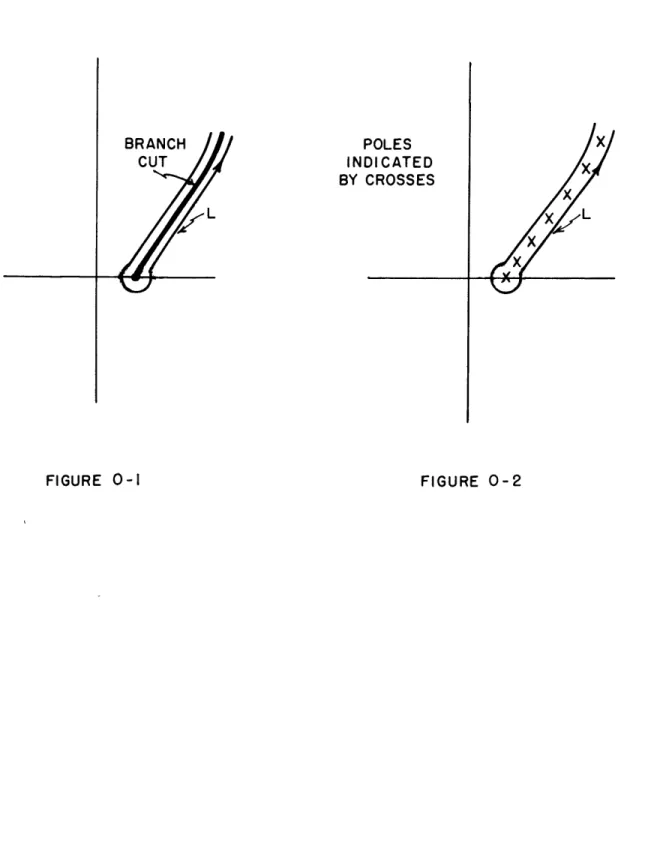
where L is the lancet contour of Figure 0-1. The singularities of g(z)
are outside of this contour,whereas f(z) has a branch cut inside the
contour. Now by a theorem of Mittag-Lefler or a similar theorem by
Runge (see Appendix C) we can replace f(z) by a rational function
approx-imation with poles in the original branch cut position, as indicated in
Figure 0-2. We then collapse the contour L onto these poles employing
the Residue Theorem to obtain the approximation to the branch cut
inte-gral I. If the number of poles is increased indefinitely, we can cause
the approximation to converge to the true value of I. In
most practical
cases only a few poles are needed.
This method of replacing the branch cut by poles or pole-zero
chains, since there are always zeros between the poles, and then using
the Residue Theorem has been called the cliff method of integration
(CerrillO, 1953). The name comes from the fact that the surface of the
14
The principal developments of this thesis are based on research carried out since 1950 by Dr. M. V. Cerrillo of the Massachusetts Institute of Technology. His investigations showed the practicality of the developments by obtaining new forms for the solution to an electromagnetic wave propagation problem (Research Laboratory of Electronics Quarterly Progress Report, July 15, 1953). The integrals associated with wave propagation problems appeared to be well suited to the mathematical approach of these investigations. Since this
coincided with my interest in geophysics, I decided to make this my thesis area.
POLES INDICATED
BY CROSSES
16
THESIS ORGANIZATION
Chapter I is concerned with the evaluation of branch cut integrals by the cliff methods of integration. These methods are developed in detail and compared with the non-topological methods of numerical analysis.
Chapters II and III are devoted to integration methods which are primarily concerned with saddle points and steepest descent paths. Chapter II demonstrates how the cliff methods of integration can be advantageously combined with the topographic features of saddle points. Chapter III demonstrates how non-topological methods--quadrature
methods--can be used to extend the range of the well-known saddle point methods of integration. The first part of Chapter III is devoted to a review of the saddle point methods and their various modifications in
order to provide a basis for evaluating the quadrature method extension. In Chapter IV the Sommerfeld dipole radiation problem is used to illustrate the analytical steps which must be taken before applying the approximate integration methods to a wave propagation problem.
A perusal of the Table of Contents will give a more detailed picture of the organization.
Chapter I
CLIFF METHODS AND BRANCH CUTS
In this chapter the application of cliff methods of integration to branch cut integrals will be developed. The results will then be compared with the standard quadrature methods for handling these integrals. In order to employ the cliff methods, three basic steps must be taken.
First the integral to be evaluated must be put in the form
j
g(z)f(z)dz where C is a lancet contour about the branch cut(s) of f(z) and g(z) contains no singularities inside this lancet contour. Later on these conditions will be relaxed somewhat.Second, the function f(z) which is generated by branch cuts and perhaps additional singularities must be approximated by rational functions. The conditions under which this can be done and the
mechanism for finding the appropriate rational functions are given in the section on Representation by Rational Functions. One method for generating the approximations is given by the branch of analysis called continued fraction analysis. It is a logical starting point, as it is a well developed field. However for our purposes, a more general approach
comes directly from the Cauchy integral, and it is this latter method which will be developed in detail.
The third step is to replace f(z) by its rational function
18
as the original branch cut, so we can collapse the lancet contour C onto these poles. For the (simple) cliff method the integration around the poles is accomplished by the Residue Theorem. The same is true for the
"extended cliff" method to be developed in this chapter. In the section on the "general cliff" method, the integrations are performed in an entirely different manner due to the fact that the approximant to f(z) is no longer a rational function with simple poles but is a function of a rational function.
The formal basis for what follows in this chapter is to be found in the work of Borel, Hadamard, Mittag-Lefler, Weierstrass and others. For instance the Weierstrass factorization theorem for entire functions, a similar theorem for meromorphic functions by Hadamard and the Mittag-Lefler theorem on partial fraction expansions are basic. However, only a theorem by Runge (which includes the Mittag-Lefler theorem) will be necessary for an orderly development of what follows. Rather than
couch the ideas in a great deal of mathematical rigor, I have decided to make the presentation simpler by including a minimum of general theorems,
as these can be found in the references. This does not affect the methods developed or the conclusions obtained. Also much of the conciseness of formal mathematics has been sacrificed in order to make the ideas
accessible to a wider audience.
REPRESENTATION BY RATIONAL FUNCTIONS
By the theorem of Mittag-Lefler or of Runge, a function f(z) which is generated by poles, branch cuts and essential singularities can be
approximated by rational functions which, of course, have only pole singularities. Furthermore the rational functions can be made to converge uniformly to the original function. In general, we have
where h(z) is a polynomial, as the expansion in rational functions. If the sum is truncated after a finite number of terms, it is called a partial fraction expansion. The partial fraction expansion together with the polynomial form a rational function approximant to f(z). The methods for locating the poles z. and determining the coefficients a. will now be given.
The powerful methods of continued fraction analysis enable us to obtain the coefficients a and the poles z. for the rational function approximants to a large class of functions. There are quite general theorems which show when the approximants obtained by these methods converge uniformly to the original function. If the singularities of a function are branch cuts, in general the poles and zeros of the approximants will be in the position of the branch cuts. The theorems and details are given by Perron and Wall.
This approach to finding the rational function approximants to the original function is limited by a certain rigidity as to the shape and position of the branch cuts involved. A more objectionable limitation for our applications is that the positions of the poles of the approx-imants are predetermined by the method, so that in general the poles
20
are not optimally located with respect to the integration around the branch cut. Also there is no simple method for obtaining the numbers a. and z..
3 3
Now it can be shown (see Perron) that the representation given by continued fraction analysis is equivalent to a representation of the original function by Stieltjes integrals. This representation in turn is, for our purposes, a special case of a more flexible method which employs the Cauchy integral and is developed in what follows.
Since it is basic to the discussion, the Cauchy Integral Formula also known as the Cauchy Integral Theorem is repeated here. If F(z) is continuous on C and analytic interior to C then
F(Z)
z
interior to
C
c
0
z exierior
to
C
where C is the smooth boundary of a finite, finitely connected region. Generalizations and rigor are given in the references by Muskhelishvili, Plemelj and Privalov among others.
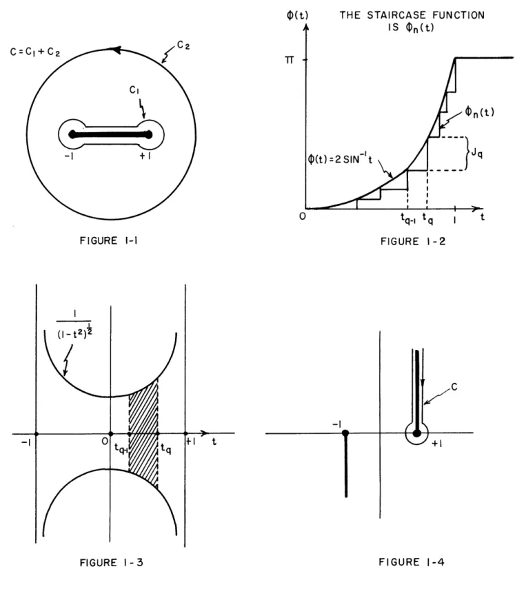
We shall now illustrate how the Cauchy Formula is applied to obtain rational approximants to a function f(z). We shall take the specific case f(z) = (1-z2) where we take the branch for which the real part of this function is positive in the upper half plane when the branch cut is chosen as in Figure 1-1. If C1 + C2 is the contour of Figure 1-1 then
(1-1)
(i zl J-
2
6
.Lj'
LYt
d'
lrit - Z iO
(|(t) THE STAIRCASE FUNCTION IS $n(t) c=ci+C c' 2
CC
On( -1+1 (t) = 2 SIN~1 t J 0 tq. t tFIGURE I-1 FIGURE 1-2
FIGURE 1-4
t)
22
The integral on C2 vanishes as the radius of the circle is extended to infinity, so that upon collapsing C1 onto the cut we are left with
where r(t) = 2sin~it. In this particular example, due to the symmetry,
we find it simpler to deal with the integration over (0,1) instead of over (-1,1). The final integral above is in the form of a Stieltjes integral where ? (t) is called the distribution function. We require the Stieltjes form because the method of approximation we shall employ
cannot be developed with just the Riemann integral. In general the distribution function is obtained by integration:
The properties of the Stieltjes integrals are described, for instance, by Widder and will not be repeated here.
In order to obtain a rational function approximant from 1-2 we approximate the distribution function
(t)
by the staircase functionf,(t)
shown in Figure 1-2. Then by the definition of the Stieltjes integral we have on substituting f, (t) into the final integral of 1-223
exact meaning of the J is clearer if we use the definition of the distribution functions to write
t
Now the function (1-z2)-T has a cliff-like discontinuity at the branch
cut from -1 to +1 on the real axis. The face of this cliff is shown in Figure 1-3. It is evident from the above integral representation that the jumps Jq are just the areas of the cliff face between pairs of poles
t and t . In the general case when the branch cuts are not on the
q
q-1
real or imaginary axes, the cliff will have a complex area so that the jumps Jq will also be complex.
The position and number of poles in the right side of 1-3 will depend on the particular application. Suppose we want to evaluate
f, g(z)(l-z2)4dz where C1 is the contour of Figure 1-1. Then the optimum position of the poles is determined by the weighting factor
g(z) and the accuracy desired. By the method of construction it is clear that we are free to place the poles where we want them as long as they are in the position of the branch cut. This is is contrast to the continued fraction analysis approach in which the pole positions are predetermined (see Perron or Wall).
Suppose that the weighting factor g(z) is such that we can take the jumps Jq of Figure 1-2 to be equally spaced so that -J
=
/N.24
(1-4)
p
~:
Jimz)~ -X> +If N is finite, the right side of 1-4 is a rational function approximant to (1-z2)d. If the limit process is carried out we obtain the function on the left as expected. In this example the jumps are equally spaced. In some problems it might be preferable to choose some other spacingor we could choose the poles t to be equally spaced. Various theorems
on convergence and estimates on the error for a given number of terms can be derived from the results of Perron.
CLIFF METHOD
The preceding section gave the mechanism for expanding a function f(z) in terms of rational functions which we shall denote by Rn(z). The theorems given Appendix C show that the R (z) can be uniformly convergent.
n
Even though these functions converge uniformly to f(z), this is no guarantee that the right hand integral of
where Rn(z) is the rational approximant to f(z) will also converge uniformly to the limit. In fact the limit may well be divergent.
Sufficient conditions for convergence can be obtained from the theorems of Appendix C. If these conditions are met, then we can make some very definite observations about the whole structure of the cliff method.
25
In 1-5 let us substitute for R (z) its general form n
where h(z) is a polynomial. Then we obtain
(1-6)
=
||
ia
n IM
/i
where J are the jumps derived from the distribution function
f(t) for
f(t). We have assumed C to be an appropriate contour such as that of Figure 1-4, so that the Residue Theorem applies at the poles of R n(z).That the a. can be replaced by J./27ri in the right side of 1-6 can be seen for the case f(z) = (1-z2)-f if we write the sum on the
right side of 1-3 in the form
(1-7)
-z--Z
i
where J = +Jq and t
=
+t q, the upper sign corresponding to j being a positive number. Then since f(z)=
lim Rn(z) = lim a/(z-tj)
+ h(z),we have ai = J /2mri on comparing coefficients. It is not hard to
generalize this, but we shall omit the proof here.
Now if we take only a few terms of the sum on the right of 1-6 we have the cliff method approximation to the integral I. The relation-ship of this approximation to the Stieltjes definition of the original integral can be seen if we replace f(z)dz by d f(z)/2] in the left hand integral of 1-5 and collapse the contour C onto the cut. We then have by a definition of the Stieltjes integral
26
(1-8)~~aj
1
d9~
I~
9
where f(t) is the distribution function for 2f(t). The sum on the right has the same form as the sum on the right of 1-6 if we remember that the jumps J were defined in terms of the distribution function for f(t) by J
=
?(t )- '(t1 ). It is clear now that the cliffmethod approximation is just a partial sum of the Stieltjes definition of the original integral along the banks of a branch cut.
Our method of approximate integration can viewed from these two standpoints. In one we replace a branch cut by a chain of poles and deform our contour of integration onto these poles. In the other, we deform our contour of integration onto the banks of the branch cut and simply use the Stieltjes definition of the resultant integrals. Since we are dealing with contour deformations and singular lines (branch cuts),
the former viewpoint is probably more natural. In the general cliff method described later, this viewpoint will be imperative. For the
cliff method and the extended cliff method of the next section, it will be helpful to think in terms of the Stieltjes integral approach as well as the purely topological approach of rational function approximants.
Before developing the extended cliff method, let us see how to apply the cliff method when we do not have a lancet contour around a cut.
Suppose the integral to be evaluated is of the form 1-5, but that the contour C only extends along one bank of the cut. As before, expand
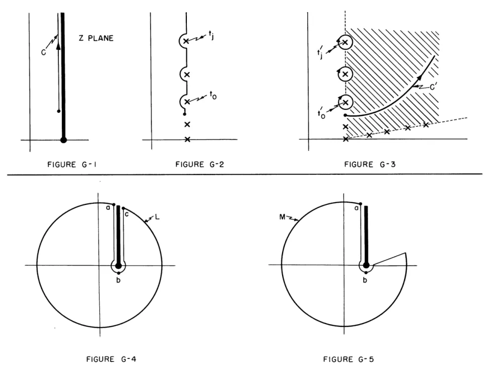
f(z) in a rational approximant with poles along the cut position. We then deform C onto these poles so that C consists of semicircles around the poles plus straight line segments between the poles. Our cliff method solution to the integral I is then given by taking one-half of the values of the residues at these poles. (If we are dealing with other than double valued functions, then the residues would be weighted differently). We neglect the contribution from the straight line
segments in our approximation. That this should be done can be seen by an appeal to the Cauchy Integral Theorem as explained in Appendix G. Another way to see this is to employ the Stieltjes integral along the bank of the cut and show that the approximation obtained in this manner gives the same result as taking half residues.
EXTENDED CLIFF METHOD
It sometimes becomes necessary, in order to obtain a good approxi-mation, to use a large number of steps in the staircase approximation to the distribution function. Then the cliff method becomes impractical. To see how this situation can be remedied, consider the general form of the cliff method solution given in 1-6. If the sum index appears in g(t ) and J.
=
f(t
)-f(t.
) in certain ways, it is possible to perform the finite summations and take the limit as the number of terms, and hence poles, become infinite. But this is redundant if, in the summation and limit, the poles become dense along the branch cut position. All we succeed in doing is to obtain the original Stieltjes integral or an28
equivalent form, since we are actually dealing with a definition of the
point
Stieltjes integral. The importantgis that if the original integral is unknown, we may be able to evaluate it approximately by replacing g(z)
and the distribution function for f(z) by approximate forms whose Stieltjes integrals are tabulated functions.
A simple example will make the ideas clearer and at the same time show the basic difference between the extended cliff method and quad-rature methods. We shall evaluate the integral representation for the Bessel function
e
Z
(1-10)
"I
jz
where C1 is the contour of Figure 1-1 and a is real.
The first step is to obtain a rational approximant to (1-z2 We start with the right hand integral of 1-2 and replace the distribution
f(t)
= 2sin~it by the straight lines shown in Figure 1-5. These two straight lines, (t) and p(t) form an approximate distribution functionet) + P(t)- f(t). The next step is to approximate 9It) and
e(t) by the staircase functions G(t) andr (t) indicated in Figure 1-5.
If we take the jumps of (t) and
f,
(t) to be equally spaced, we have J= 3/2N and J=
3/2N so that ?,t)
3q/2N and tq)=
q q q
3/2 + 3q/2N . Then we can solve for t obtaining t
=
3q/4N andq q
29
Z..2Z
7
7
If we now substitute the rational approximant on the right into 1-10 and employ the Residue Theorem, we obtain finally
(1-11)
7
(5o(co(
-e4)
1
trN IV
V )v
The extended cliff solution is obtained by letting N become infinite in 1-11. We first perform the finite summations and then take the limit obtaining
(1-12)
3c)
a
/#4
-5/
.Ira
When we let N become infinite, the stair case functions (t) and
t)
became identical with the functions
7
t
kt)
and
/t).X
Then the
only error introduced in our approximation is due to the difference between t) + (f (t) and 0(t). In other words the extended cliff method handled the function exp(iaz)of 1-10 exactly but approximatedthe integral of (1-z2)-A --that is, the distribution function. The actual error of the above approximation is a few per cent for small z.
The accuracy could be increased by choosing the ordinates in an optimum fashion or using three or four straight lines to approximate the arc sine. We could also have used the first few terms of a fourier expansion or a higher order polynomial as an approximation to the arc
0(t) A TT - 0(t) =2 SIN't IS APPROXIMATED BY THE LINES
0
(t)=2t FOR t ( 10, .75] , $ (t)fl= 6 t-3 FOR tE1.75,1] 2-I| -FIGURE 1-531
sine.
In Appendix E, Figure E-3, the approximation 1-12 is compared to a four point Chebyshev-Gauss quadrature for the integral obtained by collapsing the contour of 1-10 onto the branch cut:
(1-13)
(a)
-I
The interesting fact is that for this example, the extended cliff sol-ution compares very favorably with the quadrature solsol-ution--in fact the extended cliff solution stays with the Bessel function longer than does the quadrature.
If we had started with the integral 1-13 along the banks of the branch cut, and put it into the Stieltjes form
4T.(a)
z{c5tfs,''
we could work directly with the distribution function. We simply make the straight line approximation to the distribution function and obtain the solution 1-12. This way we do not have to consider rational function expansions or take limits as the poles become dense along the branch cut position.
We see that the extended cliff method is equivalent to dealing with the Stieltjes form of an integral along the banks of a branch cut. The distribution function is approximated by simpler functions for which the
apply a quadrature rule, the extended cliff method has the advantage of being easy to apply.
The past two sections have brought out the relation between
rational function approximants and approximations made directly to the distribution function of a Stieltjes integral. In the general cliff method section, the viewpoint of expansion in rational functions will not be equivalent to a Stieltjes integral representation.
ERROR ANALYSIS
We shall now consider the errors introduced by the cliff and extended cliff methods. First we shall examine a specific function to illustrate what happens in the cliff method from the geometric stand-point.
24-Let f(z) = (1-z ) in the left hand integral of 1-5 and let C be the contour designated by C in Figure 1-1. We shall employ the
1
expansion 1-4 and keep the number of poles finite. We have on
substituting 1-4 into the above integral and using the Residue Theorem:
where J = 7T/N . Now as shown in Figure 1-3, the jumps J are the
q q
areas of the face of the cliff for (1-z between the poles tq and t If the weight factor is unity, that is, g(z) = 1, then, exactly,
q-1.
Since the integral is just the total area of the cliff face, we need only a finite number of poles for an exact answer. In fact two poles (at z = +1) would be sufficient.
Now if g(z) is not unity it is clear that the cliff method weights the areas J by the value of g(z) at z
=
t so that g(z)is approximated by a constant between each pair of poles.
Next compare this cliff method solution with a quadrature for which f(z) = (l-z2)-I is a weight factor--the Chebyshev-Gauss formula.
In place of the crude step-like approximation to g(z) of the cliff method, the quadrature rule with, say, m points approximates g(z) by
a 2m-1 degree polynomial. This is generally a considerable improvement on the cliff method solution. However if f(z) does not have the form of a weighting function of known orthogonal polynomials, then the cliff method may be the most practical means for obtaining the approximate
solution. Moreover the method is straight forward and easy to apply. In fact as the examples of Appendix E show, the cliff method solution is not
so crude as might be thought from the above comparison.
A tight error analysis for the cliff method is quite difficult to develop. However a conservative analysis can be obtained by considering
the integral of 1-5. We have
where
jf(z)
is the distribution function for f(z). The approximation to I is given by34
where for the cliff method
9h
(z)
is the staircase approximation to
(z)
as indicated in Figure 1-2 for the case
9(t)
=
2sin
1t. The
error is then
By collapsing C onto the branch cut we can consider this to be a line
integral with limits a and b. For this line integral we shall let
z
=
t. By the partial integration formula for Stieltjes integrals we
can then express the error as
'IA
b
For the cliff method the set of points at which
f(t)-
,(t) is
discontinuous has measure zero. Also we can assume
()
(t
is bounded on [a,b]
.
Then if g(t) is continuous and monotonic, it
can be shown by the methods of functional analysis that
Also if g(t) is
merely of bounded variation on
[a,b]
and
q'(t)-9f(t)
is continuous (as it is in the extended cliff method) then we have
35
where lub means least upper bound and V denotes the total variation.
These inequalities enable us to set a bound on the error
I-In'
However these bounds are very conservative. Until a better error analysis
is developed the best that can be done is to give some numerical
exam-ples to show that the cliff method can have high accuracy with only a
few terms. These examples are relegated to Appendix E and show that
the cliff method compares quite favorably with non-topological methods
such as quadrature rules.
GENERAL CLIFF METHOD
Suppose the integral taken on the contour of Figure 1-4 has the
form
(1-14)
()
7~f
hdf7)c-C
where the branch cut surrounded by C belongs to f(z). Neither g(z)
nor hjf(z) have any other singularities inside this contour. We shall
replace f(z) by a rational function approximant with poles in the
posi-tion of the original branch cut as before. However there is now a basic
difference in our method of approximate integration from that of the
(simple) cliff methods. We are now expanding the argument of a function
instead of the complete function in rational functions. The previous
methods are the special case for h being the identity operator. In
more complicated than the simple poles we encountered previously.
To illustrate why this generalization has a practical motivation,
let h be the exponential operator so that 1-14 becomes
(1-15)
I
-fj(z)
e
az
L
Our first thought might be to apply the (simple) cliff methods
after removing f(z) from the exponential by an appropriate transformation
or to expand exp f(z) itself in rational functions. In
many cases the
first alternative is not feasible because of the complicated form of the
integrand. In most cases the latter alternative is impractical because
the methods available for obtaining a rational function expansion of an
exponential of this sort are very awkward. For these reasons it is
desireable to develop the ideas of the general cliff method.
In our example we replace exp f(z) by the approximant exp Rn(z)
which has essential singularities at the poles of Rn(z)= a/(z-z)
n
+
h(z)
.We have now replaced the branch cut by a chain of essential
singularities. When the contour L is collapsed onto these isolated
essential singularities, we have the approximation
I a;M(Z-zij *ho) aj I{z-2,)+f e(-2,) -t htz)
(1-16)
I
lim jY(z)e
dz
=
itn
dz"
L
where near any of the poles zj the functions g(z) and
am/(z-zm)
+
h(z) are nearly constant. These integrals can be evaluated by the
37
method of Appendix F. If only a few terms are needed, then we have a practical solution. Unlike the cliff methods developed previously, there is no simple relation between our approximate solution and the partial sums of the definition of a Stieltjes integral.
To illustrate the application of the general cliff method and some of its limitations, let us consider a typical integral appearing in wave propagation problems:
(1-17)
IH,
{(-P~~)d
C
H is the Hankel function of the first kind, C is the lancet contour on the left side of Figure 1-6 and we assume the singularities of g(z) are exterior to this contour. Suppose thatyA varies between .1 and 10 so that quadrature methods are awkward to apply.
The first step in the general cliff method is to expand (1-z2) in a rational function approximant Rn(z). At the zeros of this rational function, the argument of the Hankel function is zero so that Ho DRn(z)j has logarithmic singularities (logarithmic branch points) at these points. At the poles of Rn(z) the Hankel function has branch points which we
shall call essential singularities. The contour C can then be collapsed onto the singularities of He oRn(z) as shown in the right hand side of Figure 1-6. The branch cutting is that for HoaRn(z)] and does not come from the function being approximated. It seems reasonable that the whole effect of the original branch cut which generated H 0f(1-z2)ijis
O= ZERO OF Rn (U) AND
LOGARITHMIC SINGULARITY OF Ho [Rn(U)]
X = POLE OF Rn (U) AND
ESSENTIAL SINGULARITY OF Ho[Rn(U)] FIGURE 1-6 U PLANE
OX
FIGURE 1-7 U PLANE U PLANE -139
of the branch cut and not by the new branch cuts introduced for H
Rn(z)
.
Nevertheless when we collapse the contour C onto the singularities of
H
R
Rn(z),
we must consider the integrations along the banks of the cuts
for this function, as is demonstrated in Appendix F.
It now would appear that all we have succeeded in doing is to
replace a single branch cut integral by a number of new ones and have
therefor multiplied our difficulties. We shall return to this point
later, but for the time being assume that we can surmount these
difficul-ties.
We still have to consider the contributions at the branch points of
HoIR (z)] designated by 0 and X in the right side of Figure 1-6. Near
these branch points H4
0Rn(z)] can be replaced by its logarithmic or
x
asymptotic forms. Then if z are the poles and
9
are the zeros of
R (z), we have the approximation
n
{ yJR(Z )
z
(1-18)
=
Zi
+
contrib1on
of
branc
/x 0
where the loops about z and z are placed as shown in Figure 1-7. For
integrals of the type appearing in the Sommerfeld problem the integrations
about
z
vanish. The proof is straight forward. The integrations about
the
i
can be handled by the method shown in Appendix F if the angles of
the branch cuts issuing from the zj are adjusted so that the integrals
40
converge and the phase requirements of the asymptotic forms are satisfied. The problem remains of evaluating the integrals along the banks of the branch cutting for Ho R (z)] . Theoretically, though not practi-cally, it is possible to expand the original function HO (1-z ) in a
rational function approximant S n(z). Now compare this with the approximant H [R (z)J . Both these approximants are generated by their singularities.
Since both are approximants to the same function, there must be a relation between the poles of Sn (z) and the branch cuts and branch points of
H.pR (z)] . If we can find a practical relation between the integrations
around the poles of S (z) and the integrations along the banks of the n
cuts for HJ/ R (z), it may be possible to evaluate the integrals along the banks of the cuts by applying the Residue Theorem to the poles of Sn (z). It also may not be necessary to have obtained the exact form of Sn(z) first. These possibilities require careful investigation, but were considered to be beyond the scope of the present thesis and are left for future work.
In the present section we have considered two examples of the general cliff method. In the first example, the operator h of equation 1-14 was the exponential function, so that the general cliff method could be carried out. We did not give an actual numerical example, as this will be done in Appendix E. In the second example of this section, the operator h was the Hankel function. As we have seen, in this case we run into difficulties in applying the general cliff method, although more study is necessary before we can make definite conclusions.
41
SUMMARY
The present chapter has shown that both the cliff and extended cliff methods have practical applications to branch cut integrals. An error
analysis was given, but as shown in Appendix E, it is much too conservative. A tight error analysis for the cliff methods is difficult to develop.
The examples of Appendix E do show that the error can be quite small-in fact the cliff methods compare quite favorably with quadrature methods. The important observation is that the cliff methods can be applied to integrals which do not readily yield to quadrature methods either because the weight factor is not the right form or because of singular behavior of a factor of the integrand.
The general cliff method was carried to a point where it did not appear too promising for functions such as the Hankel function. The simpler example worked out in Appendix E also shows serious limitations. However more work is necessary before definite conclusions are obtained.
As explained in the example of Appendix E, the cliff method also can be applied to singular integral equations which are not readily adaptible to methods such as Gaussian quadrature.
Chapter II
CLIFF METHODS AND SADDLE POINTS
The previous chapter was concerned with the application of cliff methods of integration to branch cut integrals without any special regard to whether the integral had exponential behavior in its integrand. For many wave propagation integrals, the integrands do have a dominant
ex-ponential factor so that the main contribution to the integral comes in the vicinity of saddle points. We shall show how it is possible to combine the cliff methods with the properties of saddle points to obtain a powerful extension to the ordinary saddle point methods. The reader unfamiliar with saddle point methods will find this chapter clearer if he first reads Chapter III.
The general type of integral we shall consider has the form
(2-1)
R7e
)
e U/ (Z)
Wz
f
L
where the contour L may be of several types as discussed in what follows. We shall assume that f(z) does not contain terms of exponential order.
CLIFF METHOD--SEPARATED INTEGRAND
We shall apply the cliff method to evaluate 2-1 where we assume this integral is of the "separated" form--that is, f(z) and w(z) do not contain the same multivalued functions. For simplicity assume w(z) has
43
one saddle point as indicated in Figure 2-1 and that L is a lancet contour about a cut which belongs to f(z). The steepest descent line passing through the saddle point is indicated in the figure.
There are three ways in which we can employ the cliff method: (1) we can deform the cut together with the lancet contour L onto the steepest descent path. Then we place the poles of the rational approx-imant to f(z) in the position of this deformed cut, collapse L onto the poles and employ the Residue Theorem. Since we are on a steepest descent path only a few poles near the saddle point are needed for our approx-imation. (2) we can first deform L onto the steepest descent path so that it is an open contour. Then we deform the cut onto the steepest descent path as indicated in Figure 2-2. Next we replace the cut by the poles of the rational approximant to f(z). The approximate solution
is given by taking weighted residues at the poles.
The proper weighting and necessary assumptions are developed in Appendix G. For double valued functions we take half residues at the poles. Again we only need a few poles near the saddle point since we are on a steepest descent line. If there are no other singularities
(such as branch points of g(z) ) near the saddle point, then this is a practical method.
(3) we can first deform L as an open contour onto the steepest descent path. Then we expand f(z) in a rational approximant Rn(z) which approximates f(z) in the unshaded region of Figure 2-3. Interior to the shaded region, R n(z) becomes vanishingly small by Cauchy's Integral Theorem. The poles of Rn(z) lie along the boundary of the twc regions as
Steepest
Descent
Path
Saddle
Point
'
FIGURE
L is Equivalent To Loops
2-1
Plus L'
Deformed Onto
Steepest Descent
L
FIGURE 2-2
Branch Cuts For (-
Z2
)
-1
est Descent
FIGURE 2-4
Path
/
Path
Branch Cut
e0o.-O
FIGURE
2-3
n
45indicated. The next step is to deform L back onto the shaded region in a position such as L'. We are left with the loops around the poles on the steepest descent path (again only the poles near the saddle point are important) plus the integral on L'. In some cases, depending on w(z), L' can be shown to vanish as we deform it toward the point at infinity. Otherwise we can make the contribution from L' arbitrarily
small by taking enourh poles &ong the steepest descent path. This follows from the well-known properties of the Cauchy Integral Formula. From the form of R (z) we can set bounds on the value of the integral
n along L', if necessary.
These approaches to the integration problem are primarily topolog-ical. In practice it is easier to deform L onto the steepest descent path and then throw the integral into Stieltjes form in terms of the dis-tribution function for f(z). We then approximate this distribution
function by a stair case function as explained in Chapter I. The result will be the same as would be obtained by (2) or (3) above.
Since we can place our poles as we wish, it is possible to follow curved steepest descent paths and broad saddles.
CLIFF METHOD--MIXED INTEGRAND
Suppose that w(z) and f(z) both contain the same multivalued function--say, (1-z 2)2 with cuts as indicated in Figure 2-4. If we
deform the cut (from +1) together with the lancet contour L onto the
steepest descent path, we must expand both w(z) and f(z) before we collapse L onto the singularities of the approximant. Since a rational function
46
expansion in an exponent leads to essential singularities, we cannot employ the (simple) cliff method. However, if we deform L as an open contour on the steepest descent path, we can use the cliff method as follows.
Suppose that the integrand of 2-1 contains a number of multivalued functions. We can consider the Riemann surface rendering this integrand single valued to consist of sheets each of which is subdivided into two leaves corresponding to the two branches of (1-z2)i. Now we can expand this subdivision into four sheets, two of which correspond to
(1-z2) in f(z) and two of which correspond to the (l-z2)$ in w(z). In other words, we consider these as different functions, although they have the same branch points.
Then to apply the cliff method, we remember that we are on one sheet of our four sheeted subdivision. We deform the cut for the (1-z2)i belonging to f(z) onto the steepest descent path. Then we expand the (1-z2)$ of f(z) in a rational function which approximates
(1-z2) in the unshaded region of Figure 2-5. We next deform L back into the shaded region. We are left with the residues at the poles on the steepest descent path plus the contour L' which has wrapped around the cut belonging to the (1-z2)f in the exponent.
Nbw note that we could have expressed our integral in Stieltjes form along the steepest descent path, so that the distribution function would be generated by f(z). If we then approximate this distribution
function in the usual manner with a stair case-like function, we obtain the same approximate solution as we would from the rational function
The Contour L is Deformed
Plus The Branch Cut
Onto The Poles
FIGURE 2-5
Steepest Descent Paths For
Jo(Z)
+ 7r
Saddle Points
Are At w=0,7r
48
approach described above. The only difference between the two procedures is that the more topological approach gives some idea of the error that the integral on L' will introduce whereas the Stieltjes integral approach does not consider this.
EXAMPLE OF CLIFF METHOD
As a numerical example, consider the representation of the Bessel function
(2-2)
e
Y
where Yis the contour of Figure 2-6 and is already on the steepest descent paths for the two saddle points. In this case we can transform our integral into a line integral along the steepest descent paths. The result is the integral 'I of equation E-1 of Appendix E. In Table E
the result of approximating this integral by the cliff method is
compared with the solution obtained by the ordinary saddle point method. For reference, the saddle point method solution is
(7.- )Cos
(z
)
At least up to z = 4Th the cliff method with five poles gives more accurate results. For z (/4 the cliff method is not too good
(although it does not blow up as does the saddle point method solution). For small z, if it were desireable, the cliff method solution could be easily improved by choosing a different pole spacing.
GENERAL CLIFF METHOD
Suppose that w(z) contains the function (1-z2) with the cuts as shown in Figure 2-4. Then we have the choices: (1) we can deform the cut from +1 together with its lancet contour L onto the steepest descent path and employ the general cliff method. (2) we can deform L as an open contour onto the steepest descent path and expand w(z) in a rational function Rn(z) which approaches w(z) in a region as indicated by the unshaded area of Figure 2-3. Then exp Rn(z) has a ring of essential singularities around this unshaded region. exp R (z) approaches exp w(z) interior to the unshaded region and approaches unity in the shaded region. This can be proven from Cauchy's Integral Theorem and the theorems of Appendix C. Next we deform L onto the singularities along the steepest descent path--again we need only those near the saddle point--plus a contour L' in the shaded region. If the poles of R (z) are close enough then exp Rn(z) f(z)dz approaches f(z)dz
which may be easier to evaluate.
SUMMARY
The cliff method provides an important extension to the saddle point methods because, as shown in this chapter, the method can handle broad
saddles and curved steepest descent paths. These are just the cases in which the ordinary (asymptotic) saddle point methods break down.
Because of the difficulties described in the section on the general cliff method of Chapter I and in Appendix E, the application of this method to steepest descent paths is not yet very practical.
Chapter III
SADDLE POINT METHODS
The preceding chapter brought out the power of the cliff methods of
integration when applied to steepest descent paths. In this way the cliff
methods provide a powerful extension to the popular saddle point method of
integration, known also as the method of steepest descents and the
sta-tionary phase or col method, depending on the application. In
this
chap-ter another means of extending the ordinary saddle point method will be
given. Basically this extension is the application of quadrature methods
to steepest descent paths and will be called the quadrature saddle point
method. A review of the ordinary saddle point method and some of its var-iations will first be given in order to make the presentation clearer.
The general type of integral handled by the saddle point method is
F(t)=SFS)e
ds
where L is the contour of integration in the complex s plane, F(s) and
W(st) are analytic functions on this contour and t denotes any parameters.