Local Community Detection in Multilayer Networks
Texte intégral
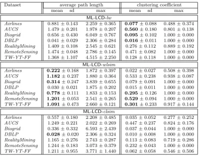
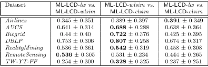
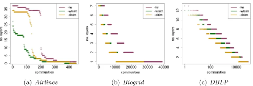
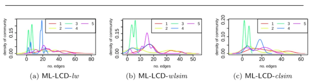
Figure


Documents relatifs
In Section 5, we give a specific implementation of a combined MRG of this form and we compare its speed with other combined MRGs proposed in L’Ecuyer (1996) and L’Ecuyer (1999a),
(https://orcid. of São Paulo, São Paulo, Brazil. de Biologia, Univ. Federal do Rio de Janeiro, Rio de Janeiro, RJ, Brazil. NACM also at: Programa de Pós-Graduação em Ecologia,
De plus, de nombreux répondants nous ont dit qu’il faudrait offrir les services réduction des méfaits dans différents milieux (hôpitaux, pharmacies, centres de
With respect to the local, the two key ideas Pennycook develops in his book are the notion of relocalisation as a broader and more dynamic concept than recontextualisation, and
The goal of this paper is to investigate LOSCs by looking into their role in open source development, what challenges and benefits they bring or face and what interaction patterns
L’archive ouverte pluridisciplinaire HAL, est destinée au dépôt et à la diffusion de documents scientifiques de niveau recherche, publiés ou non, émanant des
The direct simulation of the mechanical behavior of polycrystalline aggregates based on crystal plasticity provides a wealth of information about the development of strain
In the pooled results and the 1962–1982 census years, the further apart two departments are, the more different is their share of Saint names.. The re- ported coefficients
