SEPTEMBER 1988 LIDS-P-1830
Analysis of Gain Scheduled Control for
Linear Parameter-Varying Plants'
Jeff S. Shamma Michael Athans Room 35-409
Laboratory for Information and Decision Systems Massachusetts Institute of Technology
Cambridge, MA 02139 (617) 253-5992
Abstract
Gain scheduling has proven to be a successful design methodology in many engineering applications. The idea is to construct a global feedback control system for a time-varying and/or nonlinear plant from a collection of local linear time-invariant designs. However, in the absence of a sound analysis, these designs come with no guarantees on the robustness, performance, or even nominal stability of the overall gain scheduled design.
We present such an analysis for one type of gain scheduled system, namely, a linear parameter-varying plant scheduling on its exogenous parameters. This class of systems is important since it can be shown that gain scheduled control of nonlinear plants takes the form of a linear parameter-varying plant where the "parameter" is actually a reference trajectory or some endogenous signal such as the plant output. Conditions are given which guarantee that the stability, robustness, and performance properties of the fixed operating point designs carry over to the global gain scheduled design. These conditions confirm and formalize popular notions regarding gain scheduled designs, such as the scheduling variable should "vary
slowly."
Keywords: Gain Scheduling, Time-Varying Systems, Robust Stability, Nonlinear Design, Delay Systems.
1 This research was supported by the NASA Ames and Langley Research Centers under grant NASA/NAG 2-297.
Submitted to: Symposium on Nonlinear Control Systems Design, Capri, Italy, June 1989 and AUTOMATICA.
Section 1. Introduction
1.1 Problem Statement
Gain scheduling (e.g., [31]) is a popular engineering method used to design controllers for systems with widely varying nonlinear and/or parameter dependent dynamics, i.e., systems for which a single linear time-invariant model is insufficient. The idea is to select several operating points which cover the range of the plant's dynamics. Then, at each of these points, the designer makes a linear time-invariant approximation to the plant and designs a linear compensator for each linearized plant. In between operating points, the parameters (i.e., "gains") of the compensators are then interpolated, or "scheduled," thus resulting in a global feedback compensator.
Despite the lack of a sound theoretical analysis, gain scheduling is a design methodology which is known to word in a myriad of operating control systems (e.g., jet engines, submarianes, and aircraft). However, in the absence of such an analysis, these designs come with no guarantees. More precisely, even though the local operating point designs may have excellent feedback properties, the global gain scheduled design need not have any of these properties, even nominal stability. In other words, one typically cannot assess a priori the guaranteed stability, robustness, and performance properties of gain scheduled designs. Rather, any such properties are inferred from extensive computer simulations.
This paper addresses this issue of guaranteed properties for one class of gain scheduled control systems, namely, linear parameter-varying plants. This class of systems is important since it can be shown that gain scheduled control of nonlinear plants takes the form of a linear parameter-varying plant where the "parameter" is actually a reference trajectory or some endogenous signal such as the plant output (cf. [36]). One example of a physical system whose (linearized) dynamics take the form of (1-1)-(1-2) is an aircraft, where the time-varying parameter is typically dynamic pressure (e.g., [32]).
Consider a plant of the form
x(t) = A(O(t)) x(t) + B(O(t)) u(t) (1-1)
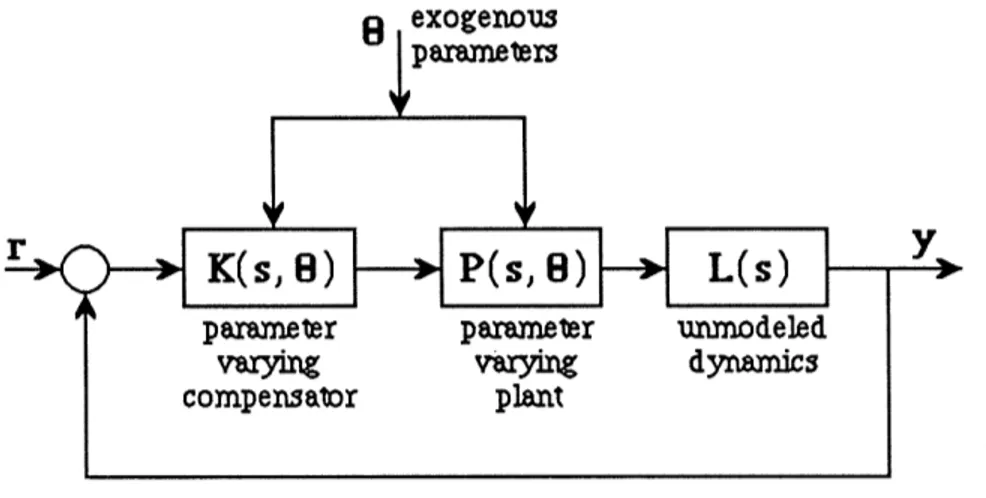
These equations represent a linear plant whose dynamics depend on a vector of time-varying exogenous parameters, 0, which take their values in some prescribed set O(t) E O. Gain scheduled controllers for such plants typically are designed as follows. First, the designer selects a set of parameter values, {0i}, which represent the range of the plant's dynamics, and designs a linear time-invariant compensator for each. Then, in between operating points, the compensators are interpolated such that for all frozen values of the parameters, the closed loop system has excellent feedback properties, such as nominal stability, robustness to unmodeled dynamics, and robust performance (Fig. 1-1).
8 exogenous parameters
r K(s, 8) DO P(s, 8); L(s)
parameter parameter unmrodeled
varying varying dynamics
compensator plant
Figure 1-1 A Linear Plant Scheduling on Exogenous Parameters
Since the parameters are actually time-varying, none of these properties need carry over to the overall time-varying closed loop system. Even in the simplest case of nominal stability (i.e. no unmodeled dynamics), parameter time-variations can be destabilizing.
In this paper, conditions are given which guarantee that the closed loop system will retain the feedback properties of the frozen-time designs. These conditions formalize various heuristic ideas which have guided successful gain scheduled designs. For example, one primary guideline is "the scheduling variables should vary slowly with respect to the system dyna-mics." Note that this idea is simply a reminder that the original designs were based on linear time-invariant approximations to the actual plant. In this sense, these approximations must be sufficiently faithful to the true plant if one expects the global design to exhibit the desired feedback properties. In fact, it is this idea which proves most fundamental in the forthcoming
-2-analysis.
The remainder of this paper is organized as follows. This section closes with the mathematical notation to be used throughout the paper. Section 2 addresses the issue of nominal stability. In Section 2.1, the mechanism of time-varying instability arising from frozen-time stability is discussed. Section 2.2 discusses the general problem of stability of slowly-varying linear systems. In Section 3, the issues of robust stability and robust performance are addressed. The formal problem statement is given in Section 3.1. Section 3.2 presents background material on Volterra integrodifferential equations. In Section 3.3, conditions are given which guarantee time-varying robustness/performance given frozen-time robustness/performance. The conditions are presented from both a state-space and input-output viewpoint. Finally, concluding remarks are given in Section 4.
1.2 Mathematical Notation
A+ denotes the set { t E R I t 0 }. I * I denotes both the vector norm on Rn and its induced matrix norm.
Let f: k + -- > R n. f denotes the Laplace transform of f. P T denotes the standard truncation operator on f. WTa denotes the truncation and exponential weighting operator on f defined by
e- f(t), t<T
(WT,a f)(t) =
0D
,
t>T
Lp and Lpe, p E [1, oo], denote the standard Lebesgue and extended Lebesgue function spaces. Similarly, lp, p E [1, oo], denote the appropriately summable sequence spaces. B denotes the set of functions such that
IIf lIIB sup If(t) I < 00
+ tE
Be denotes the set of functions such that P f E B, V T E R+ .
-3-A(a) denotes the set whose elements are of the form f(t) = t 0 t0, t<O wherefa: A+ - - , ti > 0, f E A, and o0aoti IfllA-- - If (t) e I dt + f i e i< oo 0 i=0
For any two elements of
A
(a), f* g denotes the convolution of f and g. Anxm(a) denotes the set of n by m matrices whose elements are in A(u). Let A E Anxm(a) and letA' E Rn x m as 'ij =A-II Aij IA(a). Then define II A 11A(a) - A' I. Finally, A(a) and
Anxm(c) are defined as the set of Laplace transforms of elements of A(a) and Anxm(a), respectively. For further details on A(a) and ,(a), see [5, 11].
-4-Section 2. Nominal Stability
2.1 The Mechanism of Time-Varying InstabilityEven in the simplest case of nominal stability, it is well known that time-variations can destabilize a frozen-time stable system. For example, consider the linear system [1, 34].
[X1(t)
1
[-a sin 2t -a cos 2t 1 X(t)1
_ =
dtX2(t)
--a cos 2t
a sin 2t
x2(t)
(2-1)where a is a constant parameter. The eigenvalues of the dynamics matrix are given by a-2±+ a_ 4
"
12=a- +2 (2-2)
1,2 2
which are constant and lie in the left-half complex plane for all a < 2. However, the state transition matrix is given by
(t,)=
(a -1) t -t (2-3)-e sin t e cost
Thus, it is seen that for the values of a, 1 < a < 2, the time-varying dynamics of (2-1) are unstable, even though the frozen-time dynamics are stable. Conversely, reference [30] contains an example where the time-varying dynamics are stable, while the frozen-time dynamics are unstable.
This instability phenomena can be explained as follows. Although the frozen-time systems are stable, each frozen-time trajectory experiences a certain amount of amplification in norm of the initial conditions before the state decays to zero. Thus, instability occurs when the time-variations are introduced in such a way that the time-varying state trajectory always experiences these amplification phases.
-5-2.2 Stability of Slowly Varying Systems
Suppose that one has carried out the gain scheduled design procedure outlined in the introduction for some linear parameter-varying plant. Then along any particular parameter vector trajectory, the closed loop unforced dynamics are of the form
x(t) = A(t) x(t), x(O) = xo E an, t 2 0. (2-4)
where A now represents the closed loop dynamics matrix.
In this section, conditions are given which guarantee time-varying stability of (2-4) given frozen-time stability. In relation to the gain scheduled design, these conditions can be used to place restrictions on the nature of allowable parameter variations in order to guarantee nominal stability. These conditions summarize and extend previous results found in [10, 11, 22, 33]. Furthermore, the approach taken here extends almost immediately to the analysis of time-varying robustness and performance.
First, assumptions on (2-4) and a preliminary lemma are presented.
Assumption 2-1 The dynamics matrix A: R+ -- Rn xn is bounded and globally Lipschitz continuous with constant LA, i.e.
I A(t) - A(r) I < LA I t- l r Vt, e R+. (2-5)
Lemma 2-1 [2] Consider the linear system
x(t) = Aox(t) + 6A(t) x(t), x(0) = xo E R , t 2 0. (2-6)
Suppose that for some m, A, and k > 0
I eAot I < me-at, (2-7)
I A(t) I < k, V t 0. (2-8)
Under these conditions,
I x(t) I < me- ( -mk) t X I V t 0, x
0 E n . (2-9)
Proof The solution to (2-6) is given by
-6-Ao(t) t Ao(t- )
x(t) = e x +
J
e SA(x) I x(r) I d (2-10)0 Using (2-7) and (2-8),
t
Ix(t) I <me Ix I + me- it)klx() Idsr (2-11)
Multiplying by e-
At
and applying the Bellman-Gronwall inequality,I x(t) I < me-O-mk)tl x I. (2-12)
The usefulness of Lemma 2-1 is that it allows one to guarantee exponential stability of a perturbed time-varying system (2-6) given that the unperturbed time-invariant system (SA(t)
0) is exponentially stable
The main result of this section is now presented.
Theorem 2-1 Consider the linear system of (2-4) under Assumption 2-1. Assume that at each instant in time (1) A(t) is a stable matrix and (2) there exist constants m and
A2
0 such thatIe A()t I < me- At V t, zr 0. (2-13)
Under these conditions, given any )7 e [0, A],
LA < (-/)2 (2-14)
A 4mln m
implies
I x(t)l < me- nt t t , X n (2-15)
Proof Consider approximating A(t) in (2-4) by the piecewise constant matrix
Apc(t) - A(nT), nT < t < (n+l)T, n =0,1,2,... (2-16)
where T is to be chosen. Rewriting (2-4),
-7-x(t) = Apc(t) -7-x(t) + {A(t) - Apc(t) -7-x(t). (2-17) Now choose
T 2 m (2-18)
Then for all time t > 0,
I A(t)- Apc(t)I• LAT < 27 (2-19)
where LA is chosen according to (2-14). It follows from Lemma 2-1 that on nT < t <
(n+l)T, - (t - nT) Ix(t) I < me I x(nT) I (2-20) rl (t - nT) 2 T n < m e me Ixo ,- r7 (t - nT) - T me-te 2 {me 2 }n xl0 < m e- 77't I
which completes the proof. U
Remark 1 The particular value in the condition (2-14) results from some flexibility in choosing the interval T in (2-16). This flexibility is exploited in (2-18) where the interval T is chosen to maximize the RHS of (2-15).
Remark 2 The exponential stability constants m and A in (2-13) can be calculated in a straightforward manner. For example, if the matrix A in x(t) = A xis a stability matrix, then it is easy to show that
1/2
x(K) 1
u(Q)
I x(t) I< (K) exp 2 max(K)J (2-21)
au (K) I - a
-8-where K, Q > 0 are solutions to the Lyapunov equation
KA + ATK = -Q (2-22)
Theorem 2-1 states that a time-varying system retains its frozen-time exponential stability (to a lessened degree) provided that the time-variations are sufficiently slow. It is stressed that the only restriction Theorem 2-1 imposes on the dynamics is on the rate of the variations. That is, the variations themselves may be large - provided that the dynamics change slowly. In terms of the original problem of a parameter-varying linear system, this means that the range of parameter variations may be large provided that the time derivative (e.g. with p parameters)
dA(e(t)) |A(O(t) - (t)
)
+.
+ A((t))(2-23)
k de P de
is small.
Conversely, Theorem 2-1 is not immediately applicable in the case of rapidly varying dynamics over a small range; in which case, Lemma 2-1 is more appropriate. In the case of rapidly varying dynamics over a large range, it may be possible to combine Theorem 2-1 with the method of averaging (e.g., [19, 23]) to decompose the dynamics into a "slowly-varying averaged part " and a "perturbation part."
A key parameter of the frozen-time exponential stability is the "overshoot parameter" of (2-13). For example, in the special case where m = 1, one has that the time-variations may be arbitrarily fast. This is in agreement with the discussion in Section 2.1. Recall it was stated that instability may arise when time-variations are introduced in such a way that the time-varying trajectory always experiences an amplification phase of a frozen-time trajectory. When m = 1, none of the frozen-time systems experience any amplification; hence, instability cannot occur.
Given the above explanations behind time-varying instability arising from frozen time stability, it becomes evident how possible conservatism can arise. The sufficient condition given by (2-14) prevents any "cascade of amplification phases" by uniformly enforcing that the amplification of all the frozen-time systems be sufficiently small in relation to the system's speed of response. However for time-varying instability to occur, it is required that a certain amount of "directional coincidence" of the amplification phases be present. In other words, it is possible that the frozen-time systems may exhibit a great deal of overshoot but not in such a
-9-way to cause this cascade of amplification phases. This is demonstrated by the damped Mathieu equation [35]
d2y dy
2Y + 0.2--y + (0.01 + a)y + (3.2 cos 2t)y = 0 (2-24)
which becomes unstable for a E [2, 3] and then for a > 5.
Despite the possible conservatism of Theorem 2.1, it still can be used to add new insights into gain scheduling beyond that of "schedule on a slow variable." For example, it does reveal an important point which traditionally has been ignored in gain-scheduled designs. Namely, the selection of state variables in the realization of the compensator is crucial. More precisely, suppose that one has designed a linear time-invariant compensator K(s, 0) for each value of the parameter. The notation K(s, 0) is used to stress that such designs are typically done with an emphasis on the input/output frequency domain aspects of the compensator. Now let two realizations of the compensator be given by
Xk= A(8) xk + B(0) z (2-25)
u = C(A) xk (2-26)
and
Wk = T(8) A() T- 1(0) wk + T(0) B(0) z (2-27)
u = C(O) T- (0) wk (2-28)
Although each realization results in the same frozen-parameter compensator K(s, 0), they result in two different parameter-varying compensators. To see this, note that the term T(0) T- 1(0) wk is missing in the RHS of (2-27) which would then make the two realizations time-varying equivalent. Given that the exponential stability constants of (2-13) can be extremely sensitive to the scaling of state variables, it may be that an alternate realization of the frozen-parameter compensators could mean the difference between parameter-varying stability or instability. Hence, the selection of the realization of the frozen-parameter compensators is crucial.
-10-Section 3. Robust Stability and Robust Performance
3.1 Problem StatementIn the previous section, it was shown that the nominal stability of frozen-parameter gain scheduled designs can be lost in the presence of parameter time-variations. However, if the parameter time-variations are sufficiently slow then nominal stability is maintained.
In this section, the issues of guaranteed robustness and performance in the presence of parameter time-variations are addressed. As in the case of nominal stability, given a frozen-parameter design with desirable robustness and performance properties, these properties may be lost since the parameters are actually time-varying.
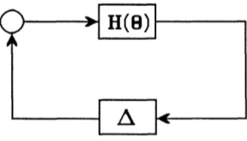
To set up the problem, consider the block diagram of Fig. 3-1. In general, any linear system with linear uncertainties, such as unmodeled sensor/actuator dynamics or even artificial uncertainties which represent performance specifictions, can be transformed to the form of Fig. 3-1 where H(O) represents a stable finite-dimensional parameter-varying linear system and A represents a block diagonal linear system which depends on only the uncertainties.
Given the block diagram of Fig. 3-1, one can use various analysis tools (e.g. small-gain theorem [6, 13] or #-value [12, 29]) to guarantee robust stability and robust performance for any frozen parameter values. However, this analysis is insufficient since the parameters are actually varying. Since the uncertainties are possibly infinite-dimensional (e.g. time-delays, flexible structures, etc.), one cannot use the state-space tools of Section 2 - hence the need for new stability tests.
Figure 3-1 General Block Diagram for Robustness / Performance Analysis
-Let H(O) have the following state-space realization
x(t) = A(0(t)) x(t) + B(0(t)) e(t) (3-1)
y(t) = C(0(t)) x(t) (3-2)
Furthermore, let the I/O relationship of A be given by
t
y'(t) = A(t- r) y(v) dr (3-3)
0 Then, the feedback equations are
t
x(t) = A(O(t)) x(t) + J B(O(t)) A(t- r) C(0(r)) x(r) dr (3-4)
0
This equation represents a type of linear Volterra integrodifferential equation (VIDE). As in the case of nominal stability, it will be shown that the stability of (3-4), hence the robustness and performance properties, are maintained in the presence of parameter time-variations provided that the variations are sufficiently slow.
3.2 Volterra Integrodifferential Equations
Before time-varying robustness and performance are discussed, some facts are presented regarding equations of the form in (3-4). Evaluating (3-4) along any parameter vector trajectory, one has that
t
x(t) = A(t) x(t) +
J
B(t) A(t- r) C(r) x(T) dT (3-5)0
where A, B, and C have been appropriately redefined. This is the general form of time-varying VIDE's and will be the object of all of the forthcoming analysis. Note that any conditions imposed on (3-5) can be translated immediately into conditions on the parameter-varying (3-4). It was stated that equation (3-5) falls under the class of linear VIDE's. In fact, under assumptions to be stated on A, (3-5) actually represents a combination of VIDE's and linear delay-differential equations. Thus, both types of equations are treated under the same framework. VIDE's and their stability have been studied in, for example, [4, 16, 17, 18, 26,
12-27, 28], and delay-differential equations in [9, 15, 20].
In this section, assumptions on (3-5) are given, a definition of exponential stability is introduced, and a sufficient condition for exponential stability in the case of time-invariant A, B, and C matrices is presented. Finally, a perturbational result analogous to Lemma 2-1 is presented.
Consider the VIDE
t
x(t) = A(t) x(t) + B(t) A(t - 1) C(r) x(r) dr, t > to (3-6)
0 with initial condition
x(t) = (t), 0 < t < to,
(
E Be (3-7)I
x(to ) = ,(to )Note that an initial condition for (3-6) consists of both an initial time, to, and an initial
function Q. Typically, the only case of interest is to = 0. However, the concept of an initial
function is quite useful in analyzing the stability of (3-6). The following assumptions are made on (3-6):
Assumption 3-1 The matrices A R+ -R n x n , B : + - R n xmf , and C AR + > p x n
are bounded and globally Lipschitz continuous with constants LA, LB,and Lc, respectively.
Assumption 3-2 For some a > 0, A E Amxp(-o).
Assumption 3-2 states the the uncertainties A are finite-gain stable as operators from L, to Loe. In the case of a rational A, this is equivalent to requiring that A is bounded and analytic in the complex RHP, Re[s] > -a, e.g. A E H° in case at = 0. In the case of infinite-dimensional A's, Assumption 3-2 is slightly stronger (see [3] for an example where A
E H° and does not satisfy Assumption 3-2).
VIDE's containing an integral operator as in Assumption 3-2 have been studied in [7, 8,
13-25], and references contained in [9]. Reference [7] establishes existence and uniqueness of solutions in the case of invariant A, B, and C matrices. Existence in the case of time-varying A, B, and C matrices is similarly shown using standard contraction mapping techniques, and is omitted here. It is noted, however, that these proofs rely heavily on Assumption 3-2. However, this assumption is not-at-all necessary for actual existence and uniqueness, e.g. the case where A is rational.
In the case of time-invariant A, B, and C matrices, solutions to (3-6) can be explicitly characterized as follows:
Theorem 3-1[7, 8] Consider the VIDE t
x(t) = A x(t) + j B A(t- I) C x(T) d + f(t), t > to (3-8) 0
x(t) = (t), 0 < t < to, Ee (3-9)
X(to ) = (to )
under Assumptions 3-1 and 3-2. Here, f E Loke is an exogenous input. In this case where A, B, and C are constant matrices, the unique solution to (3-8) is given by
t
x(t + to) = R(t) x(to) + f R(t- :) { f(r+ to) + F(r+ to) } d:, t > 0 (3-10) 0
where
to
F(t+ to) = B A(t + to - ) C ¢(t) dr, t > 0 (3-11) 0
and R is the unique matrix satisfying
R(t) = I + A R(c) + t B A(re- v) C Rm(a) d, dr , t > 0, R(O+) = I, (3-12)
The matrix R is called the 'resolvent matrix,' and is analogous to the standard matrix
-14-exponential. Note that (3-12) implies that R satisfies almost everywhere
t
R(t)=AR(t)+JB A(t- )CR( ) d, t > O (3-13)
0
A definition of exponential stability for (3-6) is now introduced. Note that the integral operator in the RHS of (3-6) depends on all of the previous values of x and not just the current value x(t). For example, it is possible that although x(to) = 0, the solution x(t) O0 for all time. This memory in the dynamics prevents one from using the standard definitions of exponential stability.
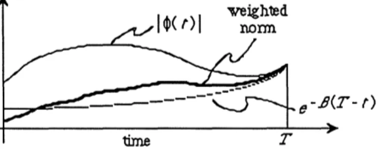
Definition 3-1 Let WT,a be defined as in Definition 2.2-7. The VIDE (3-6) is said to be exponentially stable uniformly if there exist constants m, A, and /3 > 0 where
3
2 >such that
I x(t) I meA(t >) t2, t > t ,t o E k, V E B e (3-14)
It is stressed that the constants m, A, and
1
are independent of to and q. weighednom< e- 8(2- t) Figure 3-4 Visualization of
Figure 3-4 Visualization of II WT q II1
This definition implies that not only does the state decay exponentially but also with a magnitude which is proportional to an exponentially weighted supremum of the initial function q (Fig. 3-4). This weighting essentially introduces the notion of a forgetting factor in the
15-dynamics of (3-6). That is, the value of the initial function at t << todoes little to effect the
state dynamics. The convention /8 2> A follows from the reasoning that solutions to (3-6)
cannot decay faster than they are forgotten. This convention is in agreement with the case of no integral operators in the RHS (i.e. ordinary differential equations).
The following theorem gives a sufficient condition for exponential stability in the case where A, B, and C are constant as in (3-8).
Theorem 3-2 Consider the VIDE t
x(t) = A x(t) + j B A(t- r) C x(r) dT, t > to (3-15) 0
T
xWt) =
¢(t),
0 < t < to, O' E e0 · 9EBE e )=~(i), O~r~f~ (3-16) [ x(to ) = 0(to )
A sufficient condition for uniform exponential stability is that there exist a constant P > 0 such that
s -> (sI- A - B A(s) C)1 E A (-2p8 (3-17)
mxp
A E M (-25) (3-18)
Proof It is first shown that the resolvent matrix R is bounded by a decaying exponential. Taking the Laplace transform of (3-13) shows that
R(s) = (sI - A - B A(s) C) 1 (3-19)
It follows by hypothesis (3-17) that R E Anxn(-2]3). Since R contains no impulses, R E L1, and hence R E Lf1 from (3-13). These two imply that R E L£. Now, write R as
R(t) = R'(t) eft (3-20)
Clearly, R' E Anxn(-P). Using the same arguments as above along with
-16-t
iR'(t)= (A+fI)R'(t)+J BA(t-x))C e t-R'(R )d , t > to, R'(0+) =I (3-21) 0
it follows that R and R e L1, hence R' E LO,. Thus from (3-20), it follows that there exists a
constant kl, for example II RI RIL', such that
I R(t) I < klel t Vt > 0 (3-22)
Now, recall that the solution to (3-15) is given by
t x(t + t) = R(t) x(to) + R(t - r) F(r+ to) dr, t > 0 (3-23) 0 where to F(t + to) = BA(t + to- ) C 4(t) dl, t > 0 (3-24) 0
It is now shown that F is also bounded by a decaying exponential. Rewriting (3-24),
t:+t o-T) -3(t + tq-q:) F(t + to) = B A(t + t- ) e C e () dd (3-25) 0 e 0 (tt |3B + to -'er) C - (to -r) t + t- ) CB e A(t C (v) dr (3-26) 0
Since A e Amxp(-2/P), it follows from (3-26) that there exists a constant k2 > 0, for
example k2= I B I II1 A (_ I C I, such that
I F(t + to) k2e 1IIWt l (3-27)
Substituting (3-22) and (3-27) into (3-23),
17-Ix(t
+
to) I < kle- Pt x(t) I +J klet k2e-TII W II dr (3-28) 0< kl { + e} e 11 Wto , 11 (3-29)
Since (3-29) is true for arbitrary q and to, it follows that (3-15) is uniformly exponentially
stable. U
Regarding the hypotheses of Theorem 3-2, it seems that condition (3-17) is also necessary. This is because exponential stability implies that R itself decays exponentially. Thus, R E Anxn(-2p) for some p > 0. Condition (3-17) immediately follows since it deals with the Laplace transform of R. In the case of no integral operator, i.e. A = 0, condition (3-17) reduces to the standard statement that the eigenvalues of A lie in the open complex LHP. Otherwise, it is worth noting that 'A is a stable matrix' is not assumed in proving the exponential stability of (3-15).
As for condition (3-18), note that it is slightly stronger than the standing Assumption 3-2. Specifically, Assumption 3-2 guarantees only that A E 3AP(0), and it was stated that this is
used in the existence and uniqueness proofs in [7]. As is the case for the existence and uniqueness proofs, condition (3-18) is not necessary for exponential stability. Once again, one can easily find a counterexample in the case where A is rational.
Theorem 3-2 is novel in that it takes a state-space approach, rather than input-output, to the robustness of time-invariant linear systems. This approach was chosen since it corresponds to the original motivation of parameter-varying gain scheduled systems, as in (3-4). Nevertheless, the standard results on robustness can be obtained from the previous theorem. Rewriting R(s) in (3-19),
R(s) = ( I - (sI- A)1 BA(s)s) C) (sI- A)-1 (3-30)
-18-Now suppose that A is a stable matrix; thus s f- (sI - A)-1 E Anxn(-2J,) for some
13
> 0. Assume further that A E Amxp(-2,f). Thus,s -- (I - (sI- A)1 B A(s) C ) E nxn(- 2,) (3-31) Under these conditions, R e A"mx(-2fl) if and only if [11, 21]
inf det( I - (sI - A) B A(s) C ) = det( I- C(sI- A) B A(s) ) > 0 (3-32) Re[s] >-23
However, a sufficient condition for (3-32) is that
I C [(-2 +jco)I - A] B A(-2fp+jwo) I < y < 1, V o E R (3-33) As /3 - 0, condition (3-30) approaches the standard small-gain robustness condition for time-invariant linear systems. However, unlike previous results, Theorem 3-2 gives some quantitative indication of the degree of robust stability.
Recall that the original motivation for studying VIDE's is that these equations that arise in the analysis of robustness and performance. Therefore, it is important that one is able to verify the conditions (3-17)-(3-18) for exponential stability.
First, consider condition (3-18). This assumption is stronger than requiring A to be a stable linear time-invariant system. More precisely, (3-18) implies that the impulse response of A decays exponentially with a rate of at least -2p3. This may be given the following physical interpretation. Let the mapping A': Lpe - Lpe be defined as
t
(A'u)(t) A(t - T)e ( t u() d' (3-34)
0
Then (3-18) is equivalent to the mapping A' being finite-gain stable for any p E [1, oo]. In terms of the original A, rewriting (3-34) gives
t
(A'u)(t) = e t A(t - r)e' 2'fu(:T) dz (3-35) 0
Thus, it is seen that the operator A' may be decomposed as follows: (1) Multiply the input u be a decaying exponential:
-19-u'(t) = e 2ft u(t) (3-36) (2) Pass the modified input u' through A
(3) Multiply (Au')(t) by a growing exponential:
(A'u)(t) = e 2it (Au')(t) (3-37)
Then condition (3-18) is equivalent to the sequence of operations described in (3-35)-(3-37) mapping u -- A'u being finite-gain stable for any p E [1, oo]. In case A is rational, this amounts to A not having any poles in the complex RHP, Re[s] > -2/3. Otherwise, A E ~A7XP(-2p) must either be assumed or somehow verified experimentally. This is discussed5
further in Section 3.3.
Now consider the condition (3-17). Recall that this stated the Laplace transform of the resolvent matrix R should satisfy
=nxn
R=s
t
(sI - A - B A(s) C) e a. (-2/3) (3-38) In order to verify (3-38), first let the matrix A have no eigenvalues in the complex RHP, Re[s] > -2/3, for some /3 > 0. This is in agreement with the gain scheduled case since the linear system H in (3-1)-(3-2) is designed to be stable for every frozen value of the parameter. Second, let A satisfy the condition (3-18), namely A E Amxp(-2Tj). Then using the same reasoning as in (3-30)-(3-32), R satisfies (3-38) if and only ifinf det( I - (sI - A)1 B A(s) C ) = det( I - C(sI - A)B A(s) ) > 0 (3-39) Re[s] > -2f5
which, under these conditions, is equivalent to
infdet{ I- C[(-2, +jco)I- A] B A(-2/ +jco)
}
> 0 (3-40) Now, condition (3-17) is in the form where it can be verified using standard tools from linear time-invariant robustness analysis. For example, suppose that A has been normalized [14] such thatI A(-2/3 + jo) I < 1, V c) E R. (3-41)
-Then one can use either of the following two methods to verify (3-40):
Small-Gain Condition[6, 13] Let A satisfy (3-41). Then a sufficient condition for (3-40) is that
-1
I C [(-2p3+ jo)I- A] B I < y < 1, V coE R (3-42)
]u - value[12] It turns out that in the combined analysis of robustness and performance, the uncertainty A is typically block-diagonal (e.g., [12]). In this case, one can use the gu-value nonconservatively to determine (3-40). More precisely, in case A can be any I/O stable linear time-invariant system which satisfies (3-41), a necessary and sufficient condition for (3-40) is that
u( C [(-2]3+jco)I- A] B) < 7 < 1, V oe R (3-43)
To summarize, satisfying the conditions for exponential stability (3-17)-(3-18) would require the following knowledge about A. First, knowledge of the degree of I/O stability
A E AmXP(-22 ) (3-44)
and second, a bound on A off of the jo-axis, e.g. for some 1(c),
I A(-2f + jo) I < 1(o), V w) e . (3-45) It is stressed that neither of these two may be inferred from the more common jow-axis bound on A
I A(j)o) I < l(ao), V 0 e (3-46)
(consider multiplying A any all-pass filter with a stable pole of magnitude < 2p3). This inadequacy of (3-46) is discussed further in Section 3.3.
Before closing this section, a perturbational theorem which is analogous to Lemma 2-1 is presented. Informally, this theorem states that an exponentially stable time-invariant VIDE maintains its exponential stability in the presence of sufficiently small (possibly time-varying and/or nonlinear) perturbations.
-21-Theorem 3-3 Consider the VIDE t x(t) = A x(t) + f B A(t - ) C x(:) d + (gx)(t), t > to (3-47) 0 x(t) = 0(t), 0 < t < t, E 1De (3-48) ~X~i)=~T), O0t~o.4EBe (3-48)
I
x(to )= )(t o)Here, g represents an integral operator on x. Let
s - ( sI - A - B CA(s) n. (-25) (3-49)
mxp
AeA A (-2P) A (3-50)
hold true. Assume further that there exist constants k > 0 and a >
1,
where /3 is from (3-49)-(3-50), such thatI (gx)(t) I < k 11
Wtl
a x11,
t > 0,V x E Be (3-51) Let k1be as in (3-22). Under these conditions,k < / (3-52)
k1
implies that (3-47) is uniformly exponentially stable.
Proof Define z(t) - x(t + to). As in (3-10)
t z(t) = R(t) z(O) +
J
R(t - r) { F( + to) + (gx)(r) } dr, t > 0 (3-53) 0 where to F(t + t) = BA(t+ t - ) C (t) d, t > 0 (3-54) 0As before, there exist k1 and k2 > 0 such that
I R(t) I < kle (3-55)
-22-I F(t + to) I < k2e- fII Wt, p B (3-56) Substituting (3-55), (3-56), and (3-51) into (3-53),
I z(t)I < j kle- t- ) {k2e 1 W II +k W + ke- x } d I z(0) 1 (3-57) 0
Since a > /3,
I z(t) I < J kle- 13(t- ) {k2e- 11 W Oi 11 +k I W x B } d + kle-t I z(0) I (3-58)
0 $t 0fl 1j r+ t.ji
Using Definition 2.2-7 of the truncation and exponential weighting operator,
-/T.+ to- 4)
II W xl- sup le- x( ) I (3-59)
0+r' E [0, + to ]
-fX(t°-¢) -t°- ¢(I)
~< e- PT suple
4)(A
)1 + suple ) I0E [0, to] 5E [to, + to]
Thus
t
eltt I z(t) I < k {1 + (k + k2)t} 11 W to , 4 II +
I
k k sup I e/4 z(6) I da (3-60) 0 E [0, t]Since the RHS of (3-60) is a nondecreasing function of time,
t
sup I eXPz(~) I < kl{l + (k+k2)t} II Wto) ,P 1t +fk 1k sup I eX z(Q) I d (3-61)
¢E [0, t] 0 E [0, t]
Rewriting (3-61),
t
f(t) K1+ + 2 K3J f(:) dr (3-62)
0
where,
Y1,
K2, Kc3, and f are defined in the obvious manner. Applying the Bellman-Gronwall inequality to (3-62),-f(t) < (K + -2 .}e K2 (3-63) 'CK3 'CK3
Thus,
I z(t) I < [k1 + I + -e Pkk)t [ + k ]e PIa } (3-64)
Uniform exponential stability then follows from (3-52). V
Note that (3-64) implies that for some mk (which depends on k, k1, and k2),
- (P - klk)t/2 (3-65)
Ix(t+ t0) I mke II t lB (3-65)
However, mk should be defined carefully so that as k -- 0 (i.e. as g -4 0), one has that
mk -1 k 1 + (3-66)
which is the case in (3-29) where g = 0.
3.3 Robustness and Performance of Slowly-Varying Linear Systems
In this section, the results of Section 2 are extended to VIDE's. Namely, it is shown if the VIDE (3-7) is exponentially stable for all frozen values of time, then the time-varying VIDE is exponentially stable for sufficiently slow time-variations. In terms of the original motivation of guaranteed properties for gain-scheduled control systems, this means that robustness to unmodelled dynamics and robust performance in the sense of Figs. 3-2 and 3-3 is maintained provided that the parameter variations are sufficiently slow.
Consider the VIDE
t
x(t) = A(t) x(t) + B(t) A(t - r) C(T) x(r) dr, t > t, (3-67)
with initial condition
-24-s ) = Oe(3-68)x(t
L
X(to
)= ,(t
o)Before proceeding with the theorem, some assumptions and definitions are given.
Assumption 3-3 There exists a constant /3 > 0 such that
r1 ssn +
s F-* (sI- A(r) -B() A(s) C(v)) 1E A. (-2/), V re 1 (3-69)
/A EA (-2/) (3-70)
This assumption guarantees exponential stability for all frozen values of time.
Definition 3-2 From Assumption 3-1, let kB and kc satisfy
IB(t) I < kB, Vte A+ (3-71)
I C(t) I < kc , V t E A+ (3-72)
Then define
K - LA + LB II A 11IA(_) kC + kB II A IIA( L (3-73)
Essentially, K is measure of the rate of time-variations in (3-67), i.e. as K -- 0, (3-67) approaches a time-invariant VIDE.
Definition 3-3 Let R,' denote the resolvent matrix of (3-21) associated with the frozen matrices A(r), B(r) and C(r). Then define
K1-sup 11 II hR '1 II (3-74)
+ z L~,,
K2 - kB il A IIA(_l ) kC (3-75)
These constants represent worst case values of their x-frozen analogs in (3-22) and (3-27).
-The question of slowly time-varying stability of linear VIDE's is now addressed. -The proof closely follows that of Theorem 2-1.
Theorem 3-4 Consider the VIDE (3-67) under Assumptions 3-1 and 3-3 and Definition 3-2 and 3- Under these conditions, given any tr E (0,
13),
(3-67) is uniformly exponentially stable with a decay rate of r7/2 for sufficiently small K, or equivalently, sufficiently slow time-variations in A, B, and C.Proof Let tn denote to+ nT, where T is some constant interval to be chosen. As in the
proof of Theorem 2-1, the VIDE (3-67) first is analyzed on the intervals t, < t < tn+l. Approximating A, B, and C be piecewise constant matrices, one has that
t t~
J
B(t) A(t - r) C(r) x(r) dr + (gnx)(t) 0 where t(gnx)(t) = [ A(t) - A(t) ] x(t) + f [ B(t) - B(t) ] A(t - r) C(tn) x(t) dr + (3-77)
t
jB(t) A(t- r) [ C(r) - C(t) ] x(r) d t~
Then
I (gnx)(t) I < KT II W xl < t < t+l t (3-78) Thus using Theorem 3-3, it is seen that if
KT •<
13
(3-79)2K then
-K
2 (t-tn) 2 +7)(t-t)/2 - Kt)
I x(t) <{
Kl + 1 + [ +. +.1
e J II xW x (3-80) or as in (3-65) (t - tn) 2 2 Ix(t) I < m Ke 2W2p l (3-81)In order to guarantee (3-79), choose
4 ln mK
T = (3-82)
3-Vn
K < 8 _ q) (3-83)
8 K1 In mKT
Now, (3-81) implies that
1 P+ri T
2 2
11 W x il < mKT e ! 11 W X 11W (3-84) Substituting (3-82) and (3-84) into (3-81),
2 2 -1 -(t -) 2 )-to ) )T x(t) < mK e m e
j
1Wto, It - a (t- to ) < mKTe W t o, II ~~~t 0 4i.'P~~~~ ~(3-85)which completes the proof. U
Remark It is noted that Theorem 3-4 can be extended in a straightforward manner to address
time-varying unmodeled dynamics of the form A(t, r) = G(t) A'(t - r) H(4).
-The idea behind -Theorem 3-4 is essentially the same as in the case of time-varying nominal stability. That is, the time-varying VIDE (3-67) is approximated by piecewise constant VIDE's (3-76) which are exponentially stable. Thus on each interval, the time-varying VIDE is decomposed into a constant part and a time-varying perturbation. Using Theorem 3-3, the solution will decay provided that the constant approximation is sufficiently accurate. Furthermore, this approximation must remain valid long enough to guard against any overshoot in the next interval, which is guaranteed for sufficiently slow approximations. Once again, a key parameter is the measure of overshoot mkT. In case mkT = 1, then stability is guaranteed for arbitrarily fast time-variations.
As in the case of nominal stability, the conditions one needs to check in order to verify time-varying robustness/performance are (1) the frozen-time systems are stable and (2) the time-variations are sufficiently slow. In the case of nominal stability, both of these conditions may easily be checked by examining the time-varying dynamics matrix A. However, the presence of the integral operator A makes matters more complicated.
First of all, one must verify the frozen-time stability conditions of Assumption 3-3
1 nxn +
s H-4 (sI - A(r) - B(r) A(s) C(,)) E a (-2/), V se C (3-86)
AE A (-2/3) (3-87)
As discussed in Section 2, this requires knowledge about (1) the degree of !/O stability of A for (3-87) and (2) some bound on A off of the jo -axis for (3-86). Furthermore, neither of these can be inferred from the more common assumption of ajw)-axis bound on A.
In the absence of a priori knowledge of (3-86)-(3-87), these conditions somehow must be verified experimentally. In Section 2, the I/O exponential stability of A was given a physical interpretation in terms of exponentially modified inputs and outputs to A ( see the discussion for (3-34)-(3-37) ). This interpretation stated that the I/O exponential stability of A is equivalent to the finite-gain stability of the operator
t
(A'u)(t) = e t A(t- r)e u() d(3-88) 0
Informally, this interpretation may be used to verify (3-86)-(3-87) as follows:
-Frozen-time Stability Verification
(1) Inject sufficiently rich signals u which decay exponentially at a rate of -2p into A. (2) Multiply the output from (1) by a growing exponential with rate 2/3.
(3) Obtain the operator norm of A' (if it exists). In case II A' II does not exist, then A does not have I/VO exponential stability of degree of 2/,. In terms of a rational A, this means that A has a stable pole with a real part > -2fl. It is stressed that even if II A' II does not exist, all physically realized signals remain bounded since A is stable and the multiplication of (2) is only computational.
(4) Using methods from system identification (e.g. [24]), obtain a bound on the frequency response of A'. This corresponds to the desired bound on the frequency response of A off of thejco-axis. One can the use the methods discussed in Section 2, namely the small-gain condition or tt -value, to verify (3-86).
In addition to verifying the frozen-time exponential stability, one must guarantee that the time-variations are sufficiently slow. From (3-83), this means that
K < (3-89) 8 K1 In mKT where K -LA + LB II A IIA( kc + kB 11 A IIA(_/ Lc (3-90) and mKT depends on K1- sup 11 IR ' II (3-91) + P. K2 = kB II A ilA(_) kc (3-92)
Thus, in addition to the bounds and Lipschitz constants of A, B, and C, one needs (1) the operator norm 11 A 11A(./
-(2) the time-domain bound II t F- e fit R(t) IIL .
The operator norm in (1) can be found using the frozen-time stability verification described above (with
a
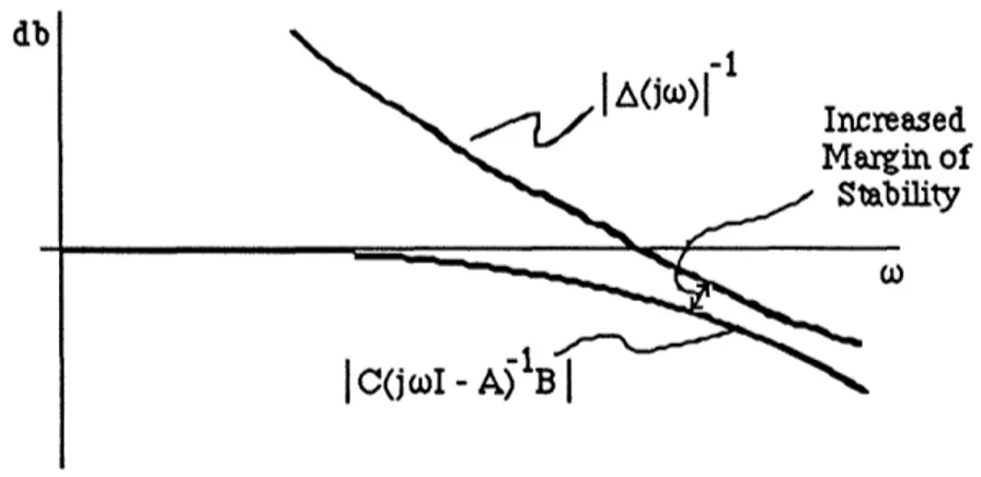
replacing 2p5). Similarly, since this procedure guarantees exponential stability, it may be used to show that the time-domain bound (2) is finite. Unfortunately, however, it does not seem possible to use this procedure to obtain even an upper bound on (2). This imposes a major restriction on the immediate applicability of Theorem 3-4.In light of these difficulties in verifying the exact conditions of Theorem 3-4, it seems that one is limited to making qualitative statements regarding guaranteed robustness and perfor-mance properties for parameter-varying gain scheduled systems. Nevertheless, Theorem 3-4 still provides useful insight into the design of these systems. Namely, it is shown that if one wants increased time-varying robustness/performance guarantees, then the frozen-time robustness tests should be met with increased margin (e.g. Fig. 3-5, where the frozen-time stability test is the small-gain condition). Qualitatively, a larger margin implies increased exponential stability of the frozen-time VIDE's which implies greater margin against time-variations.
db
Increased Margin of
Stability
Figure 3-5 Increased Stability Margin with Small-Gain Condition
All of the aforementioned difficulties regarding verification of exponential stability can be avoided by using the more classical I/O small-gain approach. However, it will be shown that even the small-gain theorem suffers from verification problems. This time, the problem lies in
-the parameter-varying system H(O) ra-ther than in -the uncertainties A.
To see this, recall the block diagram of Fig. 3- The forward-loop operator, H(8), denotes a finite-dimensional parameter-varying linear system which is frozen-time stable; the feedback-loop operator, A, denotes a possibly infinite-dimensional stable linear time-invariant system which represents various robustness and performance requirements (as in Fig. 3-2). Let H have the following state-space realization
x(t) = A(0(t)) x(t) + B(O(t)) e(t) (3-93)
y(t) = C(0(t)) x(t) (3-94)
where (for ease of discussion) the dynamics depend on a single parameter, 0. Let 0 satisfy the following conditions
9
min < 0(t) _< max (3-95)
I 0(t) I < a, V tE a+ (3-96)
Omin', ma, and a are given constants. Finally, suppose that the uncertainty A has beenx normalized [14] so that
I A(jc) I < 1, V to E k (3-97)
Under these conditions, one can use the small-gain theorem to guarantee I/O stability for any frozen value of 9. More precisely, stability of the above feedback system is guaranteed provided that
I C(0)(jo0I- A(9))-1B(0) I < y < 1 V wE R. (3-98) which is easily verified as in Fig. 3-5.
The problem is considerably more complicated for time-varying 0. Let H(9) be the I/VO operator described by
t
y'(t) = I C(O(t)) (D (t, r) B(0(T)) y ()d 6 Jr (3-99) 0
where Do6(t, r) denotes the transition-matrix associated with a certain parameter trajectory.
Using the small-gain theorem, stability is guaranteed in the case of a time-varying 0 if
II H(0) II% < y < 1 V admissible t F-> 0(t) (3-100) In other words, in order to prove stability using the small-gain theorem, one must guarantee
-that the I/VO normsfor all time-varying operators H(8) with admissible parameter trajectories satisfy (3-100).
To summarize, although the small-gain approach to time-varying robustness/performance does not require hard-to-obtain information about the uncertainties, it does require calculation of the I/O norm for families of linear parameter-varying systems. As discussed in Section 2, even the problem of determining nominal stability for families of parameter-varying systems is highly nontrivial.
In light of these difficulties, any application of the small-gain theorem is likely to be limited to the following. Suppose that the parameter-varying linear system is known to be uniformly exponentially stable for all admissible parameter trajectories (e.g. using the methods of Section 2). Then, there exists constants m and A such that
- AO(t - '
I11 (t, ) I < me t V
V
t,>
0 (3-101) for all admissible parameter trajectories. Assuming that the matrices B and C are bounded as functions of 0, it follows from (3-100) thatII H(0) i • < mV admissible t --> 0(t) (3-102) Thus, one can use (3-102) in (3-100) to give a conservative condition to guarantee time-varying robustness/performance. This approach suffers in that it completely ignores that the feedback system of Fig. 3-3 was designed to be stable for all frozen values of 0. In this sense, it offers no new insights into controller design for parameter-varying plants.
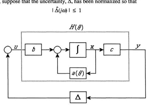
Example 3-1 This example demonstrates the use of the small-gain theorem in the simple case of a scalar system with a single parameter, and points out a limitation of the state-space approach of Theorem 3-4. Consider the scalar VIDE
t
x(t) = -a(O(t)) x(t) +
J
b A(t - r) c x(t) d (3-103) 0where a, b, and c form a state-space realization for a stable H(O) as in Fig. 3-6, and the parameter, 0, satisfies
Omin _< (t) < 0max (3-104)
32-Furthermore, suppose that the uncertainty, A, has been normalized so that
I (jO) I < 1 (3-105)
H(8)
:ZI
:
Figure 3-6 Diagram for Small-Gain Approach to VIDE Stability
Under these conditions, the small-gain theorem guarantees stability for allfrozen-values of 0 provided that
l -b <l < < 1, l Ve coe R (3-106) jo- a(O) I a(-)
As in (3-100), the small-gain theorem guarantees stability for all time-varying trajectories provided that
II H(0) IIT < < 1 V admissible t -> 80(t) (3-107) Using the definition of H(O)
t - I a(O(c)) d
y(t) = c e b u(r) dr (3-108)
0 it follows that
-cb
II H(O) Ip < Cma• y< 1| (3-109)
P oi < o< mx a(-)
Thus, the frozen-parameter stability condition (3-106) is the same as the time-varying stability criterion. In other words, the small-gain theorem guarantees that in the special case of (3-103), the parameter time-variations may be arbitrarily fast provided that the system is frozen-parameter stable for all frozen-parameter values (3-104). In terms of the previous discussion on the applicability of the small-gain theorem, the calculation of the I/O norm for a family of parameter-varying linear systems, H(8), is trivial in the scalar case of one state-variable.
It is worth mentioning here that the state-space approach of Theorem 3-4 in general will not allow arbitrary time-variations even in the scalar case of (3-103). This can be explained as follows. From condition (3-83), Theorem 3-4 allows arbitrary time-variations only if the overshoot parameter mkT = 1. In general, this is not the case for scalar VIDE's as demonstrated in the case where
1
H(s)- s 1 (3-110)
and
A(s)= 10 ( + (3-111)
(s + 14s + 14) which results in a resolvent matrix
A 1 10 -t -2t
(s) s + 2 R(t) =e + 0lt e (3-112)
(s+ + 2)2
-34-Section 4. Concluding Remarks
This paper has addressed the nominal stability, robust stability, and robust performance of parameter-varying linear systems in the context of gain scheduling. The results may be summarized as follows. Essentially, it was shown that given a gain scheduled system which has excellent feedback properties for all frozen values of the parameter, these properties are maintained provided that the parameter time-variations are sufficiently slow.
In each case, sufficient conditions on the parameter time-variations were given which guarantee stability of the overall gain scheduled system. Thus, the heuristic guideline of "scheduling on a slow variable" has been transformed into quantitative statements.
In spite of the possible conservatism and difficulty of verification of these conditions, the value of the results is that they have identified the key parameters which affect the quality of the overall gain scheduled system. For example in the case of nominal stability, a key parameter is the overshoot m of the frozen-parameter designs. In identifying this parameter, new insights were obtained on how to perform the frozen-parameter designs, such as selection of the compensator realization. In the robust stability / robust performance case, it was shown that not only must one guarantee the I/O stability of the frozen-parameter designs, but also one should have some idea of the degree of internal exponential stability. In order to guarantee such exponential stability, one should either (1) evaluate frequency-domain inequalities off of the jo-axis or (2) satisfy the standard jro -axis inequalities with an increased margin of suffi-ciency.
Thus, although the stability conditions might not be explicitly verified, the insights they provide go much beyond the "slow varying" guideline. Furthermore, the sufficiency of the conditions is simply a reminder that the designs were based on time-invariant approximations to the actual time-varying plant. If these approximations are inaccurate, then one should not demand guarantees on the overall gain scheduled system.
-References
[1] J.K. Aggarwal and E.F. Infante, "Some Remarks on the Stability of Time-Varying Systems," IEEE Transactions on Automatic Control, Vol. AC-13, No. 6, pp. 722-723, December 1968.
[2] R. Bellman, Stability Theory of Differential Equations, McGraw-Hill, New York, 1953.
[3] S. Boyd and J. Doyle, "Comparison of Peak and RMS Gains for Discrete-Time Systems," System & Control Letters, Vol. 9, pp. 1-6, 1987.
[4] T.A. Burton, Volterra Integral and Differential Equations, Academic Press, New York, 1983.
[5] F.M. Callier and C.A. Desoer, "An Algebra of Transfer Functions of Distrubuted Linear Time-Invariant Systems," IEEE Transactions on Circuits and Systems, Vol. CAS-25, No. 9, pp. 651-662, September 1978.
[6] M.J. Chen and C.A. Desoer, "Necessary and Sufficient Condition for Robust Stability of Linear Distrubuted Feedback Systems," International Journal of Control, Vol. 35, No. 2, pp. 255-267, 1982.
[7] C. Corduneanu, "Some Differential Equations with Delay," Proceedings Equadiff 3 (Czechoslovak Conference on Differential Equations and their Applications), Brno, pp. 105-114, 1973.
[8] C. Corduneanu and N. Luca, "The Stability of Some Feedback Systems with Delay," Journal of Mathematical Analysis and Applications, Vol. 51, pp. 377-393, 1975. [9] C. Corduneanu and V. Lakshmikantham, "Equations with Unbounded Delay: A
Survey," Nonlinear Analysis Theory, Methods, & Applications, Vol. 4, No. 5, pp. 831-877, 1980.
[10] C.A. Desoer, "Slowly Varying System x = A(t) x," IEEE Transactions on Automatic Control, Vol. AC-14, No. 6, pp. 780-781, December 1969.
[11] C.A. Desoer and M. Vidyasagar, Feedback Systems: Input-Output Properties, Academic Press, New York, 1975.
-[12] J. Doyle, "Analysis of Feedback Systems with Structured Uncertainties," IEE Proceedings, Vol. 129, Part D, No. 6, pp. 242-250, November 1982.
[13] J.C. Doyle and G. Stein, "Multivariable Feedback Design: Concepts for a
Classical/Modem Synthesis," IEEE Transactions on Automatic Control, Vol. AC-26, No. 1, pp. 4-16, February 1981.
[14] J.C. Doyle, J.E. Wall, and G. Stein, "Performance and Robustness for Unstructured Uncertainty," Proc. IEEE Conference on Decision and Control, pp. 629-636, 1982. [15] R.D. Driver, Ordinary and Delay Differential Equations, Springer-Verlag, New York,
1977.
[16] R. Grimmer and G. Seifert, "Stability Properties of Volterra Integrodifferential Equations," Journal of Differential Equations, Vol. 19, pp. 142-166, 1975.
[17] S.I. Grossman and R.K. Miller, "Perturbation Theory for Volterra Integrodifferential Systems," Journal of Differential Equations, Vol. 8, pp. 457-474, 1970.
[18] S.I. Grossman and R.K. Miller, "Nonlinear Volterra Integrodifferential Systems with L1-Kernels," Journal ofDifferential Equations, Vol. 13, pp. 551-566, 1973.
[19] J. Hale, Ordinary Differential Equations, Wiley, New York, 1969.
[20] J. Hale, Theory of Functional Differential Equations, Springer-Verlag, New York, 1977.
[21] E. Hille and R.S. Phillips, Functional Analysis and Semigroups, Amer. Math. Soc. Coll. Publ., XXXI, New Providence, 1957.
[22] P. Kokotovic, H. Khalil, and J. O'Reilly, Singular Perturbation Methods in Control: Analysis and Design, Academic Press, Orlando, FL, 1986.
[23] R.L. Kosut, B.D.O. Anderson, and I.M.Y. Mareels, "Stability Theory for Adaptive Systems: Method of Averaging and Persistency of Excitation," IEEE Transactions on Automatic Control, Vol. AC-32, No. 7, pp. 26-34, January 1987.
[24] L. Ljung, System Identification - Theory for the User, Prentice-Hall, Englewood Cliffs, NJ, 1986.
[25] N. Luca, "The Stability of the Solutions of a Class of Integrodifferential Systems with Infinite Delays," Journal of Mathematical Analysis and Applications, Vol. 67, pp. 323-339, 1979.
[26] R.K. Miller, Nonlinear Volterra Integral Equations, W.A. Benjamin, Menlo Park, CA,
-1971.
[27] R.K. Miller, "Asymptotic Stability Properties of Linear Volterra Integrodifferential Equations," Journal of Differential Equations, Vol. 10, pp. 485-506, 1971. [28] R.K. Miller, "Structure of Solutions of Unstable Linear Volterra Integrodifferential
Equations," Journal of Differential Equations, Vol. 15, pp. 129-157, 1974.
[29] M.G. Safonov, "Stability Margins of Diagonally Perturbed Multivariable Feedback Systems," IEE Proceedings, Vol. 129, Part D, No. 6, pp. 251-256, November 1982. [30] R.A. Skoog and C.C.G. Lau, "Instability of Slowly Varying Systems," IEEE
Transactions on Automatic Control, Vol. AC-17, No. 1, pp. 86-92, February 1972. [31] G. Stein, "Adaptive Flight Control - A Pragmatic View," Applications of Adaptive
Control, K.S. Narendra and R.V. Monopoli (eds.), Academic Press, New York, 1980. [32] G. Stein, G.L. Hartmann, and R.C. Hendrick, "Adaptive Control Laws for F-8 Flight
Test," IEEE Transactions on Automatic Control, Vol. AC-22, No. 4, pp. 758-767, October 1977.
[33] M. Vidyasagar, Nonlinear Systems Analysis, Prentice-Hall, Englewood Cliffs, NJ, 1978.
[34] M.Y. Wu, "A Note on Stability of Linear Time-Varying Systems," IEEE Transactions on Automatic Control, Vol. AC-19, No. 2, p.162, April 1974.
[35] G. Zames and R.R. Kallman, "On Spectral Mappings, Higher Order Circle Criteria, and Periodically Varying Systems," IEEE Transactions on Automatic Control, Vol. AC- 15, No. 6, pp. 649-652, December 1970.
'[36] Jeff S. Shamma and Michael Athans, "Guaranteed Properties of Nonlinear Gain Scheduled Control Systems," to appear in Proceedings of the 2 7th IEEE Conference on
Decision and Control, 1988.