Analyzing the Make-to-Stock Queue in the Supply
Chain and eBusiness Settings
by
Rene A. Caldentey
Civil Industrial Engineer, Univeristy of Chile (1995)
Submitted to the Sloan School of Management
in partial fulfillment of the requirements for the degree of
Doctor of Philosophy in Management
at the
MASSACHUSETTS INSTITUTE OF TECHNOLOGY
June 2001
( Rene A. Caldentey, MMI. All rights reserved.
The author hereby grants to MIT permission to reproduce and
distribute publicly paper and electronic copies of this thesis document
in whole or in part.
Author ...
f...
SAiu t
of Management
May 1, 2001
Certified
by ...
...
Lawrence M. Wein
DEC Leaders for Manufacturing Professor of Management Science
: Thesis Supervisor
Accepted by ...-..
...
MASSACHUSETTS IINSTITUTE.. ... ... .. ... .. MASSACHUSETTS INSTITUTE OF TECHNOLOGYMAY 0 32001
Birger Wernerfelt
Professor of Management Science
Chair, Doctoral Program
IBRARIES ,, , _ASCV41\1F-Analyzing the Make-to-Stock Queue in the Supply Chain
and eBusiness Settings
by
Rene A. Caldentey
Submitted to the Sloan School of Management on May 1, 2001, in partial fulfillment of the
requirements for the degree of
Doctor of Philosophy in Operations Management
Abstract
This thesis presents two applications of the prototypical make-to-stock queue model that are mainly motivated by supply chain management and e-commerce issues.
In the first part, we consider the decentralized version of the make-to-stock model. Two different agents that we call the supplier and the retailer control production and finish goods inventory level independently. The retailer carries finished goods inven-tory to service an exogenous demand and specifies a policy for replenishing his/her inventory from the upstream supplier. The supplier, on the other hand, chooses the capacity of his manufacturing facility. Demand is backlogged and both agents share the backorder cost. In addition, a linear inventory holding cost is charged to the retailer, and a linear cost for building production capacity is incurred by the sup-plier. The inventory level, demand rate and cost parameters are common knowledge to both agents. Under the continuous state approximation that the AM/M/1 queue has an exponential rather than geometric steady-state distribution, we characterize the optimal centralized and Nash solutions, and show that a contract with linear transfer payments based on backorder, inventory and capacity levels coordinates the system in the absence of participation constraints. We also derive explicit formulas to assess the inefficiency of the Nash equilibrium, compare the agents' decision variables and the customer service level of the centralized versus Nash solutions, and identify conditions under which a coordinating contract is desirable for both agents.
In the second part, we return to the centralized version of the make-to-stock model and analyze the situation where the price that the end customers are willing to pay for the good changes dynamically and stochastically over time. We also as-sume that demand is fully backlogged and that holding and backordering costs are linearly incurred by the manufacturer. In this setting, we formulate the stochastic control problem faced by the manager. That is, at each moment of time and based on the current inventory position, the manager decides (i) whether or not to accept an incoming order and (ii) whether or not to idle the machine. We use the expected
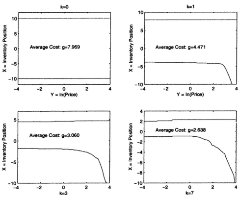
long-term average criteria to compute profits. Under heavy traffic conditions, we ap-proximate the problem by a dynamic diffusion control problem and derive optimality (Bellman) conditions. Given the mathematical complexity of the Bellman equations, numerical and approximated solutions are presented as weil as a set of computational experiments showing the quality of the proposed policies.
Thesis Supervisor: Lawrence M. Wein
Acknowledgments
I am forever and deeply indebted to the many talented people who, during the course of my life, have given me not only knowledge, but more importantly taught me the secrets behind dedication, friendship, and generosity. I cannot possibly thank here by name the full complement of those to whom thanks are owed.
First and foremost, I am extremely grateful to my advisor Larry Wein who has provided inspiration, insight, and guidance without which this thesis would never have been completed. will spend mIiy career aspiring to match the quality of his research, teaching, and advising.
The energy and courage that I have had during these years to pursue this doctoral degree come from those that I have left behind in Chile. To my brothers in arms -Rene van Kilsdonk (Bob), Ivan Marinovic (Imdn), Jorge Laval (Coco), Pedro Parra (Peter), and Rolando Cid (Rock&Rolo) with whom I grew up- I owe my curiosity for knowledge, my strong sense of friendship, and much much more. To my mentors -Don Leonardo Sanchez and Susana Mondschein- I owe my passion and love for academia. Funding was obviously important enabling me to undertake and complete this research. Without the extreme generosity of the Department of Industrial Engineer-ing of the University of Chile and the fellowship 'Beca Presidente de la Repiiblica" provided by Chilean government this work would have never been possible.
At MIT, one could not have wished to meet with a higher calibre group of persons. In particular, working with Professor Gabriel Bitran has been especially gratifying. He has not only supported my research these years with excellent advise, but more significantly he has always kept his door open to listen to my daily problems. I would like also to thank Professor Stephen Graves for his continuous and generous feedback. Over my years at Cambridge I have made a number of friends who have always been source of comfort and strength. I thank the members of the Chilean brother-hood ("Cofradia") -Fernando Ordofiez, Alejandr( Neut (Misterioso) Mario Navarro, and Pablo Garcia- for providing me the chance to periodically honor the Chilean cuisine always seasoned with friendship and unbalanced political discussion. I spe-cially thank my classmates Juan Carlos Ferrer and Ariel Schilkrlt for their unselfish academic support and for being great friends inside and outside the classroom. I deeply thank Hernan Alperin, Charles Krueger, Agneska Afelt, Machuca Ordofiez, and Ivan Mufioz for providing me all these years with the necessary escape from MIT, I will particularly miss those evenings of chess, bridge, and pool. I would like to
express my gratitude to Martin Haugh (P1..) for promoting the healthy five o'clock breaks at ABP and for lifting my personal confidence when was needed. I also thank Nicolas Stier, Brian Tomlin, Paulo Goncalves, Paulo Oliveira, Alp Muharremoglu, Ozie Ergun, John Bossert, Claudio Raddatz, Kevin Cowan, Manuel Amador, Patri-cio Mendez, Marina Zaretsky, Christian Broda, and Jremie Gallien for making MIT a friendly and much better environment.
I was particularly fortunate to have Huy Nguyen as my roommate the first year at MIT. I am specially grateful to him for making my stay at Edgerton remarkably pleasant given our proximity to Necco. I also thank my current roommates, Armida Amador (Diva), Sapna Padte, Justin Flack, and Admar Verschoor for tolerating my mess these years and for making me feel always at home.
Finally I would like to thank my family: my parents Mateo and M6nica, whose love I have never doubted, to my brothers Esteban and Eugenio who have inspired me and always provided a model for me to live up to, and to my sisters Andrea y Margarita for their care and closed contact during all these years. My final and most important acknowledgment goes to my beloved Carola for all her support and love. Beyond all doubt, her optimism and sweet smile are the only responsible for making this moment unforgettable.
Contents
1 Introduction
2 The Make-to-Stock Queue Model 2.1 Fully Backlogged Demand. 2.2 Lost Sales.
2.3 Partially Backlogged Demand. 3 A Decentralized
3.1 Introduction The Model . The Centrali The Nash Sol Comparison c Contracts The Stackelbe Proofs . . . 3.8.1 Proof 3.8.2 Proof 3.8.3 Proof Production-Inventory System 31 . . . 31 . . . 33 zed Solution ... 36 lution ... 37 )f Solutions . . . 40 . . . 45 erg Games . ... ... 50 . . . ... . 54 of Proposition 3 . . . 54 of Proposition 8 .. . . . .. 55 of Proposition 9 . . . 56 4 Revenue Management of a Make-to-Stock
4.1 Introduction ... 4.2 Literature Review.
4.3 The Control Problem ...
4.4 The Diffusion Control Problem ... 4.5 Optimality Conditions. 4.6 Numerical Solution ... 9 17 19 22 25 29 3.2 3.3 3.4 3.5 3.6 3.7 3.8 Queue . . . . . . . . . . . . . . . . 59 59 61 63 65 71 74 I . . . .
4.7 Approximations ... 4.7.1 Proposed Policy . 4.7.2 Standard Form. 4.7.3 Driftless Case. 4.7.4 General Case. 4.8 Computational Experiments. 4.9 Extensions. ...
4.9.1 Correlation Bttween Price and Demand . 4.9.2 About the Error of the Proposed Policy. 4.10 Proofs . . . . 4.10.1 Proof of Proposition (10). 4.10.2 Proof of Proposition (11) . 4.10.3 Proof of Proposition (12) ... 4.10.4 Proof of Proposition (14) . 4.10.5 Proof of Proposition (17) ... 4.10.6 Proof of Proposition (19). 5 Conclusions
A Brownian Motion and Queueing Models A.1 Introduction.
A.2 Properties of Brownian Motions ... A.2.1 Basic Properties .
A.2.2 Wiener Measure and Donsker's Theorem A.2.3 Reflection Principle .
A.2.4 Some Extensions. A.3 Stochastic Calculus.
A.3.1 Motivation . ... A.3.2 Stochastic Integration. A.3.3 It6's Lemma ... A.4 Regulated Brownian Motion ...
A.4.1 One-Sided Regulator. A.4.2 The Two-Sided Regulator. A.5 Queueing Models.
80 80 81 82 89 95 99 99 101 104 104 105 106 108 109 109 111 117 .. . . . . 117 .. . . . . 120 120 122 125 126 129 130 131 134 136 137 138 139 ... on... 139 . . . . . . . . . . . . . . . . . . . . . . . . . . . . . . . . . . . . . . . . . . . . . . . . . . . . . . . . . . . . . . . . . . . . . . . . . . . . . . . . . . . . . . . . . . . A.5.1 Introduction
CONTENTS 11 A.5.2 Single-Stage Infinite Capacity Queueing Model ... . 142 A.5.3 Single-Stage Finite Capacity Queueing Model . . . ... 146
List of Figures
2.1 The Make-to-Stock Model ... 19
2.2 Exact versus Approximate Solution ... 27
2.3 Shape of the Function H(Z) ... 28
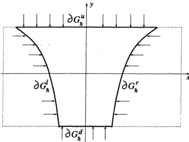
3.1 Agents' Profits as a Function of the Backorder Allocation Fraction . 39 3.2 Nash Solution as a Function of the Backorder Allocation Fraction . 44 4.1 Reflection Field at the Boundaries ... . 75
4.2 Boundary Update ... 78
4.3 Numerical Solution to the Driftless Case ... 79
4.4 Myopic Approximation vs. Numerical Solution ... 87
4.5 Proposed Policy: Driftless Case ... .. 88
4.6 Normalized Expected Average Cost ((K)) as a Function of K ... . 89
4.7 Reflection Field ... 89
4.8 Proposed Policy: General Case ... .. 95
A.1 Donsker's Theorem ... 123
A.2 Simple Process . . . ... 132
A.3 The One-Sided Regulator ... 138
List of Tables
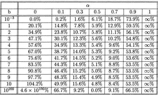
3.1 The Competition Penalty ... ... 43 4.1 Performance as a Function of the Backordering Cost Rate ... 97 4.2 Holding/Backordering cost vs. Boundary Cost ... 98 4.3 Performance as a Function of the Demand and Production Variability 99
Chapter 1
Introduction
In this thesis we study the behavior of a make-to-stock queue model under two major variations of its traditional formulation.
First, and mainly motivated by the emerging literature on supply chain manage-ment, we consider in chapter 3 a decentralized version of the make-to-stock model. Two different agents that we call the supplier and the retailer control production and finish goods inventory level independently. More precisely, we model an isolated portion of a competitive supply chain as a M/M/1 make-to-stock queue. The retailer carries finished goods inventory to service a Poisson demand process, and specifies a policy for replenishing his inventory from an upstream supplier. The supplier chooses the service rate, i.e., capacity, of his manufacturing facility, which behaves as a single-server queue with exponential service times. Demand is backlogged and both agents share the backorder cost. In addition, a linear inventory holding cost is charged to the retailer, and a linear cost for building production capacity is incurred by the sup-plier. The inventory level, demand rate and cost parameters are common knowledge to both agents. Under the continuous state approximation that the M/M/1 queue has an exponential rather than geometric steady-state distribution, we characterize the optimal centralized and Nash solutions, and show that a contract with linear transfer payments based on backorder, inventory and capacity levels coordinates the system in the absence of participation constraints. We also derive explicit formulas to assess the inefficiency of the Nash equilibrium, compare the agents' decision variables and the customer service level of the centralized versus Nash solutions, and identify conditions under which a coordinating contract is desirable for both agents.
The second variation that we consider in this work is motivated by new business practices that e-commerce is creating on the B2B and B2C markets. In particular, we believe that manufacturers and suppliers that operate on the internet are beginning to experience higher variability on the price they receive for their production. For instance, Internet price search intermediaries (web aggregators) offer customers easy access to price lists and it is just a matter of time that most consumers' purchasing decisions will be based on this type of information. On the other hand, in the Business-to-Business setting the situation is not much different. The increasing popularity of online auctions is a good example showing how spot markets are winning ground over traditional long-term fixed price contracts. For these reasons, we studied in chapter 4 a make-to-stock model where the price that customers are willing to pay for the good changes dynamically and stochastically over time. We also assume that demand is fully backlogged and that holding and backordering costs are linearly incurred by the manufacturer. In this setting, we formulate the stochastic control problem faced by the manager. That is, at each moment of time and based on the current inventory position, the manager decides (i) whether or not to accept an incoming order and (ii) whether or not to idle the machine. We use the expected long-term average criteria to compute profits. Under heavy traffic conditions, we approximate the problem by a dynamic diffusion control problem and derive optimality (Bellman) conditions. Given the mathematical complexity of the Bellman equations, numerical and approximated solutions are presented as well as a set of computational experiments showing the quality of the proposed policies.
The rest of this thesis is organized as follows. In chapter 2 we present the basic make-to-stock model and analyze some of its main properties. In Chapter 3 we study the decentralized version of the system. We analyze the non-cooperative equilibrium between supplier and retailer and we present a mechanism that allows coordination. In chapter 4 we return to the centralize model and discuss the case where the selling price behaves as a geometric Brownian motion. The admission and production control problem is formulated and approximately solved. Chapter 5 contains our conclusions. Finally, because of the use of Brownian motion processes, heavy traffic analysis, and stochastic calculus in chapter 4, we conclude this thesis with an appendix that briefly detailed the main results of these research fields.
Chapter 2
The Make-to-Stock Queue Model
In this chapter we introduce the make-to-stock model and describe its main features. The goal is to present to the reader the basic elements and properties of this simple but powerful modelling device.
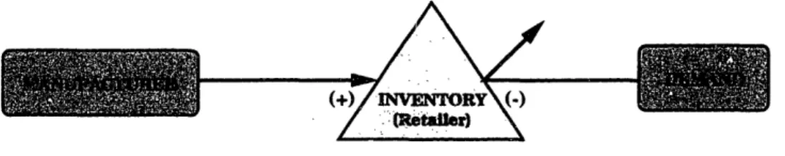
The basic make-to-stock queue model consists of three main components: (i) a demand process for a single durable good, (ii) a manufacturing facility that produces the good to satisfy the demand , and (iii) a buffer of finish goods inventory laying in between the end customer and the manufacturer. In the traditional make-to-stock model, the finish goods inventory is controlled by the manufacturer but it is also possible that a different entity owns this portion of the system. In this case, we will call (iii) the retailer's inventory. The analysis of different agents controlling the production process and the finish goods inventory is discussed in chapter 3.
The following picture schematically describe the basic element of the model. The
A/\
@
(+
W
... af-..
I )) (-)! .--- \
Figure 2.1: The Make-to-Stock Model.
plus sign in figure 2.1 indicates that the flow of finish goods coming out of the manu-facturing facility contributes positively to the inventory position. On the other hand, the minus sign indicates that the flow of demand reduces the level of stock. We now give a more detailed description of the different components of the model.
19
A
Demand is generally modelled as a renewal process with known inter-arrival time distribution fD(t) and demand rate A. We set D(t) as the cumulative demand (number of orders) up to time t and R(t) as the net revenue associated to selling one unit at time t (that is the difference between selling price and per unit production cost). In the traditional model that we will discuss in this chapter the selling price is constant over time, i.e., R(t) = R. Chapter 4 is devoted to removing this assumption considering a stochastic price process R(t).
Production, on the other hand, is modelled as a single server queueing system. We set S(t) as the cumulative production out of the manufacturer's facility up to time t. This is in general a stochastic process that depends on both (i) the service or production time of the machine and (ii) the production policy, i.e., the rule that decides when to have the machine producing or idle. Let P(t) be the production policy, that is the cumulative amount of time up to time t that the machine has been working. P(t) is a continuous and increasing process satisfying 0 < P(t) < t. We also assume here that the machine has a service time distribution fs(t) and production rate It.
Since production is capacitated, there is a natural delayed between the moment an order is placed and the moment the final good corresponding to that particular order is finally produced. In order to avoid the customer to experience this delay, the manufacturer builds a buffer of finish goods inventory . Thus, each arriving customer simply takes one unit from the finish goods inventory leaving the system without further delay instead of placing an order to the manufacturer and waiting until that order is completed. Therefore, the type of product that we consider here can not be customized, that is every customer gets the same product that the manufacturer produces and stocks. We set X as the initial level of inventory. Notice that since production and demand are both stochastic it is possible that an arriving customer sees no inventory on stock. This out-of-stock situation depends on the demand and service rate as well as in the initial inventory position and the production policy used. For instance, if the production rate is bigger than the demand rate (u > A) and the manufacturer decides to have the machine working all the time (P(t) = t) then the probability of stock out is almost zero as time goes to infinity. However, in this case the inventory of finish goods will increase systematically with time making this approach very unattractive from an economic perspective.
21 More efficient policies can be constructed in order to balance the trade-off between the probability of stock-outs and the level of finish goods inventory. Here we will discuss one particular policy that we believe is commonly used in practice and has rece.ved most of the research attention. We call this policy Re-order for each Item S'old (RIS) which is the name used by Philip M. Morse in his seminal work Queues, Inventories, and Maintenance. The main idea behind this policy is that we place an order for another unit to the factory only when one unit is sold and that the machine is working only when there are orders waiting on queue. Let X(t) and Q(t) be the level of finish goods inventory and the number of orders at time t respectively. Suppose, moreover, that at time t = 0 there is no order at the manufacturer facility (Q(0) = 0) and that the initial inventory is X(0) = X0. Then, under a RIS policy the following identity holds
X(t) + Q(t) = X0 for all t > 0.
This invariant property of the inventory position X(t) + Q(t) characterizes the make-to-stock model that we consider in this work. As a first observation, we can notice that under a RIS policy the inventory of finish good X(t) Xo ensuring that the cost of holding inventory is bounded. On the other hand, stock-out will happen when Q(t) > X0. The probability of this event depends on the particular admission policy that we consider. Three cases will be discussed here
* Case 1: Demand is fully backlogged. Every arriving order is accepted. If there is inventory on hand then the arriving customer gets immediately the product and one order for replenishment is place to the manufacturing facility. If there is no units on stock the arriving customer is backlogged until one unit of finish goods gets available for him/her. In addition, one order is place to the manufacturer. In this situation, the X(t) can be arbitrarily negative in which case the absolute value represents the number of customers waiting for the good.
* Case 2: Lost sales. Customers are accepted only if there is inventory. In this case the customer gets the good and one order is place to the manufacturer. If there is no units on stock the arriving customer is lost and no order is place to the manufacturer. We notice that in this situation X(t) is always nonnegative. * Case 3: Demand is partially backlogged. This case is a combination of the previous two. Here some customers are backlogged but there is a maximum
number of customers that can be waiting for the product. We set Xb > 0 as the maximum number of backorders. Thus, in this case we have X(t) > -Xb. Case 1 is recovered making Xb = o and case 2 is recovered making Xb = 0. From a practical point of view which of these three cases is more appropriate to use will depend on the type of market that we consider. Case 1, for instance, seems to be appropriate for a monopoly type of market where customers do not have other alternative where to go to get the product. Case 2 on the other hand reflects the situation where consumers have many buying options, thus if one manufacturer does not have the product the customer will go somewhere else to get it. Finally, case three is an intermediate situation.
From a literature perspective, the M/MA/1 make-to-stock queue was introduced by Morse (1958), but lay mysteriously dormant for the next three decades, perhaps because the multi-echelon version of it lacked the attractive decomposition property of the Clark-Scarf model and traditional (i.e., make-to-order) queueing networks, except under some restrictive inventory policies (Rubio and Wein 1996). Make-to-stock queueing systems have experienced a revival in the 1990s, including multi-product queues with (e.g., Federgruen and Katalan 1996, Markowitz et al. 1999) and without (e.g., Zheng and Zipkin 1990, Wein 1992) setups, and single-product, multi-stage systems in continuous time (e.g., Buzacott et al. 1992, Lee and Zipkin 1992) and discrete time (e.g., Glasserman and Tayur 1995 and Gavirneni et al. 1996, building on earlier work by Federgruen and Zipkin 1986).
In what follows, we will analyze in more detail the three cases mentioned above. In particular, we are interest on how to determine the optimal levels of X0 (and Xb for case 3) as a function of the different system parameters. As a general comment, we would like to mention that we have selected the average profit (cost) criteria to compute the objective function to be maximize (minimize). Thus, steady-state average profit (cost) are considered.
2.1
Fully Backlogged Demand
When demand is fully backlogged the number of orders Q(t) on the manufacturing facility is equivalent to the queue length of a single-server infinite-capacity queue-ing system. Certainly, the closed-form analysis of these systems is prohibited under general arrival and production processes. For this reason, we will focus on the
Marko-2.1. Fully Backlogged Demand
vian case, i.e., demand follows a Poisson process, production time is exponentially distributed, and both demand and production are independent.
In order to compute the optimal base-stock policy X0 2 we have to balance the trade-off between holding inventory and having customers backlogged. We notice that the- net revenue R associated to selling a unit does not play any significant role here since every order is eventually satisfied and the time average criteria is used.
On the other hand, we assume a simple linear holding/backordering cost function c(X) such that
c(X) = hX if X> O,
bX if X <O.
We can also write c(X) = hX+ + b (-X)+ where X+ = max{O,X}. Now, let Q be the number of orders in steady-state and let X be the steady-state finish goods inventory position. The existence of Q and X will be guaranteed under the Markovian assumption and the additional condition A < . Moreover, the invariant property of the make-to-stock model ensures that X + Q = X0. The steady-state average cost as a function of X0 is then given by
C(Xo) = h E[X+] + bE[(--X)+] = h E[(Xo - Q)+] + b E[(Q - X0)+]. (2.1)
Then, the problem that the manager of the production facility has to solve is to find a nonnegative integer X0 that minimizes (Xo) above. The solution of the problem is presented in the following proposition.
Proposition 1 Let Q be the steady-state number of orders being processed by the manufacturer. Then, the optimal base-stock level Xo satisfied
X0 = min{Z > 0 s.t. b < (h + b) Pr(Q < Z)}. (2.2) Proof: If X0 is the optimal base-stock level then it must satisfied the condition
E(X - 1) > (Xo) < (X 0) + 1.
2Under a base-stock policy X, the server is working as long as the finish goods inventory position
is less than Xo. When the inventory reaches the level Xo the server turns to the idle or off position.
Combining these two inequality with the identities E[(X + 1- Q)+] = E[(X - Q)+] + Pr(Q < X)
E[(Q-X)+] = E[(Q-X-1)+] + Pr(Q X + 1) for all X > 0 we get that X0 must satisfy the optimality condition
(h + b) Pr(Q < Xo- 1)-- b < O < (h + b) Pr(Q < Xo) -b. (2.3) Since the expression (h + b) Pr(Q < Xo) - b is nondecreasing in X0, condition (2.3) guarantees the uniqueness of X0. The existence is also guaranteed since lim X - ooPr(Q < X0) = 1. Finally, condition (2.2) is simply a more concise version of (2.3). i
If we forget for a moment that Q is a discrete random variable then X0 is the solution to
b Pr(Q < X) = h b
The solution is of a critical fractile type similar to those encountered on newsboy prob-lems. Thus, we just need to compute the cumulative distribution FQ(x) = Pr(Q < x) for the number of orders on the production facility. The solution is given then by
x = Fl' b
( h+b
For the moment, we have not make any particular assumption on Q rather than assuming that it has a steady-state distribution FQ(X). If we further impose the Markovian assumption we get that for the M/M/1 queue
Pr(Q < x) = 1 - p+ where p=-.
Thus, from condition (2.2) the optimal value of X is given by
X0 = [ln(h) - ln(p(h + b)) (2.4)
ln(p)
2.2. Lost Sales
with h. We can also conclude that XO = 0 is optimal if h
P-< h+b
In this case the make-to-stock system behaves like a make-to-order queue. We now turn to the analysis of Case 2.
2.2
Lost Sales
In this case we need to consider a different cost function. In particular, we do not have backordering but we do have rejections. We then assume that for each customer that is rejected because cf stock-outs the system manager incurs a penalty cost f. We recall here that for each customer that is accepted the manager received a net revenue of R. Finally, the holding cost rate for keeping finish goods on stock is again h per unit. Also, since demand is not backlogged the number of orders in the system
(Q) ranges from 0 to Xo.
In this setting, the average revenue per unit time 7r(Xo) as a function of X 0 is
given by
7r(Xo) = A R (1 - Pr(Q = Xo)) - h E[(Xo - Q)]- A f Pr(Q = Xo).
The first term is the total expected revenue obtained by selling the good, we notice that 1 - Pr(Q = Xo) is the average fraction of customers that will effectively buy the good. The second term is the expected holding cost. Finally, the third term is the expected penalty associated to rejections, here Pr(Q = Xo) is the stock-out probability.
The problem faced by the manager in this case is to find a nonnegative integer X that maximizes 7r(Xo) above. This problem was first analyzed by P. Morse (1958). In addition a quite similar but not identical problem was also studied by P. Naor (1969) in the context of socially optimal admission control to a queue. We notice that in this case, the distribution of Q does depend on the value of X0 making hard the analysis of 7r(X) without further assumption about the distribution of Q. Let us assume then that we are dealing with a Markovian system. In this case, Q is the steady-state number of order in an M/M/1/Xo queueing system and it has the
following distribution:
Pr(Q = k)
=
Ipo for all k = 0, 1,... ,X 0.I pX o+1
Proposition 2 The optimal base-stock level X0 for the lost sales case satisfies
X0 = min{Z > 0 s.t. A(R + f) < G(Z)} (2.5) where the function G(Z) is given by
1 - (Z - 2) pZ+l + (Z + 1) pZ+2 pZ (1 - p)2
We notice that G(Z) is a nondecreasing function with G(O) = 1 and G(oo) = oo. Thus, condition (2.5) is always well-defined. In addition, if A(R+ f) < h then Xo = 0 and the manager is better-off closing the production facility.
Proof: After some straightforward manipulations it can be shown that the opti-mality condition r(Xo - 1) < r(Xo) > 7r(Xo + 1) is equivalent to
(R + f) G(X),
G(Xo- 1) < h < G(Xo),
which turns out to be equivalent to (2.5). The existence of a solution is guaranteed because limx,,,G(Xo) = oo. Finally, the uniqueness is also ensured since the function G(Xa) is nondecreasing. I
Unfortunately, and mainly because of the functional form of G(Z), we can not get a closed form solution for the optimal level X0 in this case.
One possible way to get good approximations for X0 is to assume that Q is a continuous rather than discrete random variable. We can formally justify this trans-formation under heavy traffic arguments. The details of this transtrans-formation are pre-sented in the Appendix A at the end. Here, we briefly mention that for system with traffic intensity closed to unity we can approximately model the behavior of the queue length Q(t) by a regulated (one-sided or two-sided) Brownian motion. We do not pursue this approach here but we mention that the section §A.5 (and in particu-lar §A.5.3) in the appendix contains all the elements required to complete this heavy
2.2. Lost Sales
z z
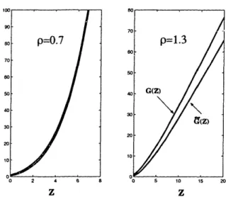
Figure 2.2: Exact versus Approximate Solution.
traffic analysis for this lost sales model.
Here, instead, we approximate X0 in a much simpler and crude way. First, we notice that the function G(Z) can be rewritten as follows
Z+1
G(Z) = (Z +
1
- k) p-kk=O
(The proof of this identity is direct and it is left to the reader). From this relation we can easily see that G(Z) is nondecreasing in Z as it was claimed above. The key of our approximation is to replace the summation by an integral. That is,
Z+l
G(Z) ~ G(Z) :=
J
(Z + 1- x)e-8 dx where 0 = ln(p). Solving the integral we gete- e(Z+l) + 0 (Z + 1) - 1
G(Z) 02
A quick comparison between G(Z) and G(Z) shows that in fact the approximation is quite accurate specially for values of p < 1. Figure 2.2 shows the behavior of G(Z) and G(Z) for two values of p. As we can see, for p < 1 the approximation is very precise. For the case p > 1 the approximation does not perform as good as in the previous case but still the prediction of Xo obtained from it are good.
H(Z)
a
H -) o H (a) Z
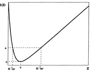
Figure 2.3: Shape of the function H(Z)
The computation of the optimal level X0 reduces to find the minimum Z satisfying A 02 (R + f)
e-@(Z+l) + (Z + 1)- 1
Let define H(Z) = exp(-Z) + Z - 1, then the approximation for X0 is given by
X0= Hl ( (R+ f)f)
-
1 (2.6)h
The shape of the function H(z) is plotted in figure 2.3. As we can see H-1(a) contains two different values for a > 0; one is positive and the other is negative. Which one of the two we will select depends on the sign of 0. If 0 is negative we select the negative value of H-l(a). The opposite is true if 0 > 0. A second order Taylor expansion of H(Z) suggest the following base stock policy.
X
0[
2(R f) 1]Notice the similarities of this solution and the standard EOQ solution (e.g., Hadley and Whitin (1963)).
As a general comment about the solution in (2.6), we can see that X0 is increasing in R and f and decreasing in h, as we should expect. It is important to notice that the impact of R and f in the optimal solution comes only through the sum R + f. Thus, low price high rejection penalty systems have the same optimal solution as high
2.3. Partially Backlogged Demand price low penalty systems.
We now turn the last of the three cases which considers simultaneously backorders and rejections.
2.3
Partially Backlogged Demand
We consider in this case that the manager has the ability to backlog as well as to reject incoming orders. In this situation, the production and admission policy is characterized by two integers X0 and Xb. X0 is the base-stock policy that controls the production. That is, the machine will be working as long as the finish goods inventory level is under X0. On the other hand, Xb is the maximum level of backorders that the system is willing/able to hold. Thus, Xb controls the admission of orders to the
system. Using the same notation that we have used in the previous two sections we can construct the expected utility per unit time for the system, r(X0,¥ X), which is given by
ir(Xo, Xb) = A R - A(R + f) Pr(Q = Xo + Xb) - h E[(Xo - Q)+] - b E[(Q- Xo)+].
In this case, Q ranges from ,...,X0 + Xb. We notice that the optimization of r(Xo, Xb) is more demanding in this case because of the two dimension. For this reason, we solve the optimization problem sequentially. First, we fix the sum L := Xo + Xb and we look for the optimal values of X0 and Xb given L. Then, we select the optimal value of L.
If we fix L, then the distribution of Q is also fixed, independent of the particular values of Xo and Xb. In this situation we get
Pr(Q = k) = p for all k = 0, 1,..., L.
l pL+1
Moreover, the first and last term in the utility function are constant and the problem reduces to minimize the holding/backordering cost
c(Xo, Xb) = h E[(Xo - Q)+] - b E[(Q - Xo)+]
subject to X0 + Xb = L. We can, in fact, rewrite the optimization problem only in terms of X0. It turns out that the optimality condition in this case with fixed L is
the same as (2.3), i.e.,
(h + b) Pr(Q < Xo -1) - b< O < (h + b) Pr(Q < Xo) - b. The optimal solution X is then characterized by the condition
Pr(Q < XolXo + Xb = L) = + b (2.7) Under the Markovian assumption, we can rewrite (2.7) as
1 - pXo+1 b ln(h + bpL+I) - Iln(h + b) - In(p)
= Xo =
1 - p+l h + b In(p)
The optimal solution is rigorously given by [Xol and Xb = L - Xo].
After some tedious algebra, the problem of finding the optimal value of L can be written as follows:
min A[(R + f) (1 -)L
L>O pL + 1)
+ h(Xo - (Xo + l)p + pX+l) + b((L - Xo)pL+2 _ (L - Xo + 1)pL+l + pX°+l)
(1 l p)(l _ pL+l)
s.t.
ln(h + bpL+ 1) - Iln(h + b) - In(p)
in(p)
Although messy, the optimization problem above is one-dimensional and it can be solved easily. We are, unfortunately, unable to compute the optimal solution in closed form. Again, we can try to use some type of approximations to estimate the optimal solutions (XO, Xb). The use of Brownian motion and heavy traffic conditions is one alternative. We postpone, however, its discussion to chapter 4 where we derive the optimal solution for this case of partially backlogged demand (see relations (4.67) and (4.68)).
Chapter 3
A Decentralized
Production-Inventory System
3.1
Introduction
Within many supply chains, a devoted upstream agent, referred to here as the sup-plier, produces goods for a downstream agent, called the retailer, in a make-to-stock manner. Broadly speaking, the performance (e.g., service levels, cost to produce and hold items) of this isolated portion of the supply chain is dictated by three factors: (i) Retailer demand, which is largely exogeneous but can in some cases be manipulated via pricing and advertising, (ii) the effectiveness of the supplier's production process and the subsequent transportation of goods, and (iii) the inventory replenishment policy, by which retailer demand is mapped into orders placed with the supplier. If the supplier and retailer are under different ownership or are independent entities within the same firm, then their competing objectives can lead to severe coordination problems: The supplier typically wants to build as little capacity as possible and re-ceive excellent demand forecasts and/or a steady stream of orders, while the retailer prefers to hold very little inventory and desires rapid response from the supplier. These tensions may deteriorate overall system performance.
The recent explosion in the academic supply chain management literature is aimed at this type of multi-agent problem. Almost without exception, the papers that incorporate stochastic demand employ variants of one of two prototypical operations management models: The newsvendor model or the Clark-Scarf (1960) multi-echelon inventory model. One-period and two-period versions of newsvendor supply chain
models have been studied intensively to address the three factors above; see Agrawal et al. (1999), Cachon (1999) and Lariviere (1999) for recent reviews. Although many valuable insights have been generated by this work, these models are primarily useful for style goods and products with very short life cycles. More complex (multi-period, and possibly multi-echlelon and positive lead time) supply chain models have been used to analyze the case where a product experiences ongoing production and demand. Of the three factors in the last paragraph, these multi-period supply chain models successfully capture the replenishment policy and have addressed some aspects of retailer demand, e.g., information lead times in the Clark-Scarf model (Chen 1999), pricing in multi-echelon models with deterministic demand and ordering costs (Chen et al. 1999), and forecast updates (Anupindi and Bassok 1999 in a multi-period newsvendor model and Tsay and Lovejoy 1999 in a multi-stage model). However, the Clark-Scarf model, and indeed all of traditional inventory theory, takes a crude approach towards the supplier's production process, by assuming that lead times are independent of the ordering process, or equivalently, that the production process is an infinite-server queue.
In this chapter, we use an alternative prototypical model, an M/M/1 make-to-stock queue, to analyze a supply chain. Here, the supplier is modeled as a single-server queue, rather than an infinite-single-server queue, and the retailer's optimal inventory replenishment strategy is a base stock policy. Because the production system is explicitly incorporated, these make-to-stock queues are also referred to as
production-inventory systems.
Much of the work done on make-to-stock queues (e.g., Wein 1992, Buzacott et al. 1992, Lee and Zipkin 1992, Rubio and Wein 1996, Federgruen and Katalan 1996, Markowitz et al. 1999, Glasserman and Tayur 1995 and Gavirneni et al. 1996) either undertake a performance analysis or consider a centralized decision maker (Gaverneni et al. analyze their systemr under various informational structures, but not in a game-theoretic setting), the make-to-stock queue is amenable to a competitive analysis because it explicitly captures the trade-off between the supplier's capacity choice and the rctailer's choice of base stock level. However, the model treats the third key factor in a naive way, by assuming that retailer demand is an exogenous Poisson process. Moreover, we assume that the system state, the demand rate and the cost parameters are known by each agent. While this assumption is admittedly crude, we believe it is an appropriate starting point for exploring competitive make-to-stock queues. In the only other multi-agent production-inventory study that we are aware of, Plambeck
3.2. The Model
and Zenios (1999), contemporaneously to us, analyze a more complex dynamic system with information asymmetry.
In an attempt to isolate - and hence understand - the impact of incorporat-ing capacity into a supply chain model, we intentionally mimic Cachon and Zipkin (1999). Their two-stage Clark-Scarf model is quite similar to our M/M/1 make-to-stock queue: Both models have two players, assume linear backorder and holding costs for retailer inventory (where the backorder costs are shared by both agents), employ steady-state analyses, and ignore fixed ordering costs. The key distinction between the two models is that the production stage is an infinite-server queue and the supplier controls his (local or echelon) inventory level in Cachon and Zipkin, whereas in our work the production stage is modeled as a single-server queue and the supplier controls the capacity level, which in turn dictates a steady-state lead time distribution. While Cachon and Zipkin's supplier incurs a linear inventory holding cost, our supplier is subjected to linear capacity and production costs. Another de-viation in the formulations is that Cachon and Zipkin's agents minimize cost, while our agents maximize profit; this allows us to explicitly incorporate participation (i.e., nonnegative profits) constraints. A minor difference is that our queueing model is in continuous time, while Cachon and Zipkin's inventory model is in discrete time. In fact, to make our results more transparent and to maintain a closer match of the two models, we use a continuous state approximation, essentially replacing the geometric steady-state distribution of the M/M/1 queue by an exponential distribution with the same mean.
The rest of this chapter is organized as follows. After defining the model in §3.2, we derive the centralized solution in §3.3, where a single decision maker optimizes system performance, and the Nash equilibrium in §3.4, where the supplier and re-tailer maximize their own profit. The two solutions are compared in §3.5. In §3.6, we describe the contract that coordinates the system; i.e., allows the decentralized system to achieve the same profit as the centralized system. In §3.7, we analyze the Stackelberg games, where one agent has all the bargaining power. Concluding remarks, on the other hand, are presented in chapter 5.
3.2
The Model
Our idealized supply chain consists of a supplier providing a single product to a retailer. Retailer demand is modeled as a homogeneous Poisson process with rate 33
A. The retailer carries inventory to service this demand, and unsatisfied demand is backordered. The retailer uses a (s - 1, s) base stock policy to replenish his inventory. That is, the inventory initially contains s units, and the retailer places an order for one unit with the supplier at each epoch of the Poisson demand process. Because we assume that there are no fixed ordering costs, the retailer's optimal replenishment policy is indeed characterized by the base stock level s.
The supplier's production facility is modeled as a single-server queue with service times that are exponentially distributed with rate . The supplier is responsible for choosing the parameter pt, which will also be referred to as the capacity. The server is only busy when retailer orders are present in the queue. The supplier's facility behaves as a M/I/1 queue because the demand process is Poisson and a base stock policy is used.
The selling price 7r that the retailer charges to the end customers and the wholesale price w that the retailer pays to the supplier are fixed. These conditions implicitly assume that the retailer and supplier operate in competitive markets. Each backo-rdered unit generates a cost b per unit of time for the production-inventory system. As in Cachon and Zipkin, this backorder cost is split between the two agents, with a fraction a E [0, 1] incurred by the retailer. The parameter a, which we refer to as the backorder allocation fraction, is exogenously specified in our model. Much of the academic literature assumes a = 1; however, even if the supplier does not care about backorders per se, he would incur a cost in switching to a different retailer if he provided extremely poor service, which suggests that this extreme case is not very realistic.
In addition, the retailer incurs a holding cost h per unit of inventory per unit of time. The supplier pays the fixed cost of building production capacity and the variable production costs. The capacity cost parameter c is per unit of product, so that c represents the amortized cost per unit of time that the supplier incurs for having the capacity ; this fixed cost rate is independent of the demand level. The variable production cost per unit is denoted by p. We assume r > w > c + p, so that positive profits are not unattainable. To make our results more transparent, we normalize the expected profit per unit time by dividing it by the holding cost rate h. Towards this end, we normalize the cost parameters as follows:
h - b Ac Ap Ar Aw
= = 1, b= , c= h p= - r = - = (3.1)
3.2. The Model
To ease the notation, we hereafter o.liit the tildes from these cost parameters.
Let N be the steady-state number of orders at the supplier's manufacturing facility. If we assume for now that > A (this point is revisited later), then N is geometrically distributed with mean v-l, where
AAh . (3.2)
This parameter, which represents the normalized excess capacity, is the supplier's de-cision variable in our analysis, and we often refer to it simply as capacity. To simplify our analysis, we assume that N is a continuous random variable, and replace the geometric distribution by an exponential distribution with parameter v. This contin-uous state approximation can be justified by a heavy traffic approximation (e.g., §10 of Harrison 1988), and leads to slightly different quantitative results (the approxima-tion tends to underestimate the optimal discrete base stock level). However, it has no effect on the qualitative system behavior, which is the object of our study.
Because the revenues for each agent are fixed, profit maximization and cost min-imization lead to the same solution. We employ profit maxmin-imization to explicitly incorporate the agents' participation constraints, which take the form of nonnegative expected profits. However, we introduce some variable cost notation (CR and Cs) in equations (3.3)-(3.4) for future reference when discussing the inefficiency of the Nash solution (§3.5) and contracts that coordinate the system (§3.6). In these equations, the quantities r - w and w - c - p are independent of the supply chain decisions (the total normalized capacity cost is Ad = c(1 + v), where c is the capacity cost if no excess capacity is built, and cv is the cost of excess capacity) and represent fixed profits for the respective agents. The steady-state expected normalized profit per unit time for the risk-neutral retailer (R) and supplier (Is) in terms of the two decision variables are given by HR(S, v) = r - w - CR(s, v) (3.3) = r-w-E[(ss-N)+] - bE[(N - s)+] 1 - e- r S e-Vs = r - w-s + - orb v v and Ils(s, V) = w-p- c- Cs(s, ) 35 (3.4)
= w-p-c-(1 - )bE[(N-s)+]-cv e-vs
w-p-c(1 + v) - (1-a)b v
3.3
The Centralized Solution
As a reference point for the efficiency of the two-agent system, we start by finding the optimal solution to the centralized version of the problem, where there is a single decision maker that simultaneously optimizes the base stock level s and the normal-ized excess capacity v. The steady-state expected normalnormal-ized profit per unit time II (defined in terms of the total variable cost C = CR + Cs) for this decision maker is
n(s, ) = IR(S, ) + Hs(s, v ) (3.5) = r-p-c-C(s,v)
= r-p-c(1 + v)-s+ 1(b +
)e-The centralized solution is given in Proposition 3; see the Appendix for the proof. Proposition 3 If r- p- c 2c cln(1 + b), then the optimal centralized solution is
the unique solution to the first-order conditions
sV =0 = vs=ln(l+b), (3.6)
11 (s, ) =
-
(b + 1)(vs s+l1) 2 + c =0, (3.7)and is given by
ln(1 + b) and s*= cln(1 + b). (3.8) c
The resulting profit is
Il(s*, v*) = r - p- c- 2/c ln(1 + b). (3.9) If r -p-c < 2/cl-n(1 + b), then the system generates negative profits and the optimal centralized solution is to not operate the supply chain.
By relation (3.6), the ratio of the base stock level, s, to the supplier's mean queue length, v-1, satisfies vs = ln(1 + b) at optimality, which corresponds to a Pareto
3.4. The Nash Solution
frontier for the selection of s and v. (The corresponding first-order conditions for the discrete inventory problem is ln(v + 1)s = ln(1 + b), and so our continuous approximation can be viewed as using the Taylor series approximation ln(v + 1) - v.) Although this ratio is independent of the capacity cost c, the optimal point on this Pareto frontier depends on c via s = vc according to (3.8).
As expected, the optimal capacity level decreases with the capacity cost and in-creases with the backorder-to-holding cost ratio b. Similarly, because capacity and safety stock provide alternative means to avoid backorders, the optimal base stock level increases with the capacity cost and with the normalized backorder cost b. Fi-nally, as expected, neither w nor ca play any role in this single-agent optimization, because transfer payments between the retailer and the supplier do no affect the centralized profit.
3.4
The Nash Solution
Under the Nash equilibrium concept, the retailer chooses s to maximize IR(S, v), assuming that the supplier chooses v to maximize HS(s, v); likewise, the supplier simultaneously chooses v to maximize rIs(s, v) assuming the retailer chooses s to maximize HR(s, v). Because each agent's strategy is a best response to the other's,
neither agent is motivated to depart from this equilibrium.
Our results are most easily presented by deriving the Nash equilibrium in the absence of participation constraints, which is done in the next proposition, and then incorporating the participation constraints, nR > 0 and ns > 0. In anticipation
of subsequent analysis, we express the Nash equilibrium in terms of the backorder allocation fraction a. Let us also define the auxilliary function
f(b) (1 ca)b(ln(l + b) + 1)(3.10) (1 + b) ln( + b)
which plays a prominent role in our analysis.
Proposition 4 In the absence of participation constraints, the unique Nash equilib-rium is
v = f(b) v* (3.11)
S* (In(l + b) )* (3.12)
The resulting profits, rI1(a) and IH(a), are
n
(a)= R(S, ,vC) = r-w-s (3.13)n(a) S = nls(s, v,) = w - w-p-c- p- c (n(l
j
In(1 IVc:) ++ ab) +
ab)+ I
cv, v (3.14) Proof: Let s*(v) be the retailer's reaction curve, i.e., the optimal base stock level given a capacity v installed by the supplier. Because (3.3) is concave in s, s*(v) is characterized by the first-order conditionvs*(v) = ln(1 + ab). (3.15) Using a similar argument, we find that the supplier's reaction curve v*(s) satisfies
eV (s)s (i/(3)s + c16)
(v(s)s)
2 / (1 - )bs2 (3.16)The unique solution to (3.15)-(3.16) is (3.11)-(3.12), and substituting this solution into (3.3)-(3.4) yields (3.13)-(3.14).
*
Because f(b) is decreasing in a and ln(1 + ab) is increasing in a for b > 0, it follows that as a increases, the retailer becomes more concerned with backorders and increases his base stock level, while the supplier cares less about backorders and builds less excess capacity.
As mentioned previously, we assume that the two agents do not participate in the game unless their expected normalized profits in (3.13)-(3.14) are nonnegative. Hence, if either of these profits are negative, the Nash equilibrium (in the presence of participation constraints) is an inoperative supply chain. The remainder of this section is devoted to an analysis of these profits as a function of a. The supplier's profit I (a) is an increasing function of a! that satisfies
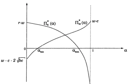
3.4. The Nash Solution 39 r-w 0 w -c -2b [ (a) , ( IWC X-, I=,0 a
Figure 3.1: The retailer's (fIR) and supplier's (Hs) profits in the Nash equilibrium as a function of the backorder allocation fraction a.
and Rn*(a) is a decreasing function of a that satisfies
fR(0)
= r - w, limlH(a)
-oo00, (3.17)as shown in Figure 3.1. (Many of the limits taken in this work, e.g., a -+ 1, are implicitly taken to be one-sided.)
To understand the unbounded retailer losses in (3.17), note that for the extreme case a = 1, the supplier does not face any backorder cost and consequently has no incentive to build excess capacity, i.e, v = 0. This corresponds to the null recurrent case of a queueing system with an arrival rate equal to its service rate, and s = oo: There is no base stock level that allows the retailer to maintain finite inventory (backorder plus holding) costs. Hence, this production-inventory system is unstable when c = 1 and the Nash equilibrium is that the retailer does not participate, and the supply chain does not operate.
More generally, there exist Cmin and am,,x such that IIH(ce) > 0 and rIH(a) > 0 if and only if c E [0amin, max]. That is, the Nash equilibrium is an inoperative supply chain when a < mi, or a > max, because one of the agents is burdened with too
much of the backorder cost. The threshold omax E (0, 1), and solves
If w - p - c 2/, then amin = 0. Otherwise, amin solves
W··=(lCl + ab) + a(b) * (3.19)
We have been unable to explicitly solve for Oma,, and amin in (3.18)-(3.19). How-ever, to increase our understanding of these two equations, we investigate the solution in two extreme cases: When backorders are much less costly than holding inventory (b << 1), we have
(r w)- 4 + 4(r
-w) 2bc- (r - w)2 (w -p-) 2 20)
Omax - 'w 2bc -min 4bc
When backorder costs are very large,
mx (r-) 2 ln(1 + b)c (3.21)
max ln(1 + b)c + (r - w)2' ln(1 + b)c + (w -p - )2
Even under the assumption r > w > c + p, it is possible that amin > amax in
(3.20)-(3.21). In this situation, even though each agent is willing to participate for some values of a, it is not possible for the retailer and supplier to simultaneously earn nonnegative profits.
3.5
Comparison of Solutions
In this section, we compare the centralized solution and the Nash equilibrium with respect to the total system profit, the agents' decisions, and the consumers of the product.
The Nash equilibrium is inefficient. As in §3.4, it is convenient to first quan-tify the inefficiency of the Nash equilibrium in the absence of participation constraints, and then to incorporate them later. In the absence of participation constraints, the centralized solution is not achievable as a Nash equilibrium. By equations (3.6) and (3.15), the first-order conditions are vs* = ln(1 + b) in the centralized solution and vs* = ln(1 + ab) in the Nash solution. Hence, the two solutions are not equal when a < 1, and the Nash equilibrium in the a = 1 case is an unstable system, as discussed earlier.
3.5. Comparison of Solutions
comparing the profits under the centralized and Nash solutions. Because the profits 7 - w and w - p - c are fixed in (3.3)-(3.4), it is more natural to restrict ourselves to the variable costs. This assumption also allows us to follow Cachon and Zipkin and compute the competition penalty, which is defined as the percentage increase in variable cost of the Nash equilibrium over the centralized solution. By (3.5) and (3.8), the variable cost for the centralized solution is
C(ts v) = - 1 eI) +b = 2+c cln(1 +b),
and the variable cost C* associated with the Nash equilibrium in the absence of participation constraints is, by (3.3)-(3.4) and Proposition 4,
C = CR(S*, v) + Cs(s, v) = [fa(b) In(1 + ab) + + ln(l + b)ib)]
In(+
ab)
+ 1 In(l + b)fa(b)Hence, the competition penalty in the absence of participation constraints is C-C(s',V') C(s' ,v) 100%, where
C,- C(s*, v*) 1 (b) n(1l +b)ab) 1
C(s*, v*) 2 (b) In(1 + b) + l n(1 + b)f(b) (3.22)
Surprisingly, the competition penalty in (3.22) is independent of the supplier's cost of capacity. This occurs because the centralized variable cost and the Nash variable cost are both proportional to /r at optimality, which is a consequence of the particular functional form arising from the make-to-stock formulation. However, this penalty is a function of ac and b, and we can simplify equation (3.22) for the limiting values of these two parameters. The function f(b) is decreasing in a and
fi (b) = 0. Hence, the competition penalty goes to oo as c - 1. This inefficiency occurs because as the retailer bears more of the backorder cost, the supplier builds less excess capacity, and in the limit the lack of excess capacity causes instability of the M/M/1 system. At the other extreme, f(b) - + a s c - 0, and the
competition penalty in this case is given by b
n(1+b) -1 for b > . (3.23) in( I b)
This function is increasing and concave in b, approaches zero as b -X 0 and grows
to oo as b - oo. Hence, when the supplier incurs most of the backorder cost, the retailer holds very little inventory and the competition penalty depends primarily on the backorder cost; if this cost is low then the supplier has little incentive to build excess capacity, which leads to a small competition penalty because the centralized planner holds neither safety stock nor excess capacity in this case. In contrast, if the backorder cost is very high, the supplier cannot overcome the retailer's lack of safety stock, and his backorders get out of control, leading to high inefficiency.
Turning to the backorder cost asymptotics, f(b) - f as b -+ o, and the competition penalty approaches
- 1. (3.24)
2Vaa(1 - a)
This quantity vanishes at a = 0.5, is symmetric about a = 0.5, is convex for a E (0, 1), and approaches oo as a - 0 and a -+ 1. Thus, when backorders are very expensive, this cost component dominates both agents' objective functions when they care equally about backorders (ca = 0.5), and their cost functions - and hence decisions - coincide with the centralized solution. However, when there is a severe imbalance in the backorder allocation (a is near 0 or 1), one of the agents does not build enough of his buffer resource, and the other agent cannot prevent many costly backorders, which is highly inefficient from the viewpoint of the entire supply chain. Finally, for the case b - 0, the competition penalty is given by
_2 - 1, (3.25)
which is an increasing convex function of a. Consistent with the previous analyses, this penalty function vanishes as ac - 0 and approaches oo as a -+ 1.
In summary, there are two regimes, (a = 0.5, b - oo) and (a -+ 0, b -+ 0), where the Nash equilibrium is asymptotically efficient, and two regimes, ae - 1 and ( -+ 0, b -4 o), where the inefficiency of the Nash solution is arbitrarily large. However, because equation (3.22) does not consider the agents' participation constraints, some of the large inefficiencies in the latter regimes are not attainable by the supply chain. To complement these asymptotic results, we compute in Table 3.1 the competition penalty in (3.22) for various values of a and b. Our asymptotic results agree with the numbers around the four edges of this table. Two new insights emerge from Table 3.1. First, the competition penalty is minimized by a near 0.5 (i.e., the backorder