HAL Id: hal-02280257
https://hal-univ-rennes1.archives-ouvertes.fr/hal-02280257
Submitted on 28 Sep 2020
HAL is a multi-disciplinary open access
archive for the deposit and dissemination of
sci-entific research documents, whether they are
pub-lished or not. The documents may come from
teaching and research institutions in France or
abroad, or from public or private research centers.
L’archive ouverte pluridisciplinaire HAL, est
destinée au dépôt et à la diffusion de documents
scientifiques de niveau recherche, publiés ou non,
émanant des établissements d’enseignement et de
recherche français ou étrangers, des laboratoires
publics ou privés.
MRI
Benjamin Henninger, Jose Alustiza, Maciej Garbowski, Yves Gandon
To cite this version:
Benjamin Henninger, Jose Alustiza, Maciej Garbowski, Yves Gandon. Practical guide to
quantifi-cation of hepatic iron with MRI. European Radiology, Springer Verlag, 2020, 30 (1), pp.383-393.
�10.1007/s00330-019-06380-9�. �hal-02280257�
MAGNETIC RESONANCE
Practical guide to quantification of hepatic iron with MRI
Benjamin Henninger1 &Jose Alustiza2&Maciej Garbowski3&Yves Gandon4 Received: 17 April 2019 / Revised: 3 July 2019 / Accepted: 19 July 2019
# The Author(s) 2019
Abstract
Our intention is to demystify the MR quantification of hepatic iron (i.e., the liver iron concentration) and give you a step-by-step approach by answering the most pertinent questions. The following article should be more of a manual or guide for every radiologist than a classic review article, which just summarizes the literature. Furthermore, we provide important background information for professional communication with clinicians. The information regarding the physical background is reduced to a minimum. After reading this article, you should be able to perform adequate MR measurements of the LIC with 1.5-T or 3.0-T scanners.
Key Points
• MRI is widely accepted as the primary approach to non-invasively determine liver iron concentration (LIC). • This article is a guide for every radiologist to perform adequate MR measurements of the LIC.
• When using R2* relaxometry, some points have to be considered to obtain correct measurements—all explained in this article. Keywords Iron . Liver . Magnetic resonance imaging
Abbreviations
DIOS Dysmetabolic iron overload syndrome
HH Hereditary hemochromatosis
LIC Liver iron concentration ME-GRE Multi-echo gradient-echo MRI Magnetic resonance imaging SIR Signal-intensity-ratio
TE Echo time
Introduction and overview
Magnetic resonance imaging (MRI) is widely recognized as the primary approach to non-invasively determine liver iron concentration (LIC). Over the past 20 years, various methods have been extensively studied and eventually introduced into routine clinical management in many centers. Nevertheless, in our experience, it seems that many radiologists are still “afraid” of this method and therefore do not use it or use it inappropriately. The likely reason for this seems to be its parently complex background and the many different ap-proaches on offer. As a result, although the benefits of MRI in the diagnosis and management of iron overload are at hand, MRI has only been included in a few clinical guidelines and recommendations [1–6] and is therefore actually not seen as a mandatory method that ought to be offered by every radiolo-gist working with MRI.
Which MRI techniques are available?
There is an easy way to get an idea or first impression of a possible iron overload in the liver with MRI: nearly every MRI protocol of the liver integrates a chemical shift sequence, * Benjamin Henninger
1 Department of Radiology, Medical University of Innsbruck,
Anichstraße 35, 6020 Innsbruck, Austria
2
Osatek, Donostia Universitary Hospital, P. Dr. Beguiristain 109, 20014 Donostia/San Sebastian, Spain
3
Department of Haematology, Cancer Institute, University College London, Paul O’Gorman Bld, 72 Huntley St, London WC1E 6BT, UK
4 CHU Rennes, Inserm, LTSI - UMR_S 1099, University of Rennes,
F-35000 Rennes, France
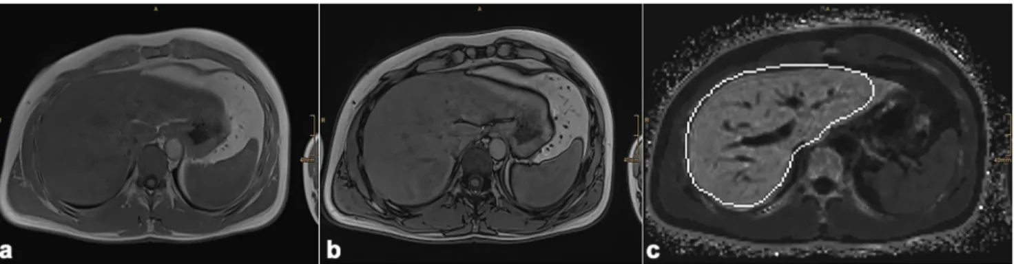
i.e., and opposed-phase. Iron leads to decreased signal in-tensity on in-phase images compared with the opposed-phase which in turn should alert on a possible iron overload disease [7,8]. An example is provided in Fig.1. A quantification meth-od has been proposed by Lim [7]. However, concomitant steatosis is a crucial limitation of this technique which compro-mises its value [9,10]. Further, fast spin-echo T2-weighted imaging can also be used to detect iron: the T2 shortening leads to low liver signal intensity, relative to that of the spleen.
There are two more advanced methods that can determine the LIC quantitatively: relaxometry and the signal-intensity-ratio method.
Relaxometry
Relaxometry is the quantitative evaluation of the MRI signal loss due to the predominant shortening of the T2 and more-over the T2* relaxation times. There are two approaches: the calculation of the T2 time constant, based on spin-echo se-quences, and of the T2* time constants, based on gradient-echo sequences. Both can be estimated from signal intensity decay acquired at multiple echo times (TEs). Because of the increase in the presence of tissue iron and therefore more logical applicability, we use the mathematical inverses of T2 and T2*, the R2 and R2* relaxation rates, for daily routine and regulatory purposes in the liver.
R2 Relaxometry - Ferriscan® (St. Pierre’s method) is a commercially available and FDA-approved technique for 1.5-T scanners, based on five T2-weighted spin-echo (SE) acquisitions during free-breathing with increasing TEs for the calculation of R2 [11]. Its advantages are undeniable showing excellent correlation with the LIC and it is used in many clinics worldwide as well as in various studies, often determined as the“gold-standard” due to its cross-site and cross-platform validation and an ongoing data quality con-trol/assurance. Nevertheless, this technique requires long im-aging time (~ 20 min), with the definitive need for sedation in pediatric imaging, complex data processing with centralized
data analysis (takes 2 business days to return a report), and a former calibration of instruments. Furthermore, a correspond-ing service fee per patient is charged with this method for the data analysis. On top of the costs of the MRI scan itself, this narrows its widespread adoption.
R2* relaxometry has emerged as a reliable method provid-ing a linear correlation with the LIC. It has shown superb reproducibility but the fact that sequence parameters and im-age analysis procedures were different among many studies has always been portrayed as a disadvantage [12–15]. Although there is no actual consensus on the ideal image acquisition, many centers are using R2* relaxometry with their house-made sequence and post-processing software with own LIC calibration. Nevertheless, studies have shown that the existing biases are correctable and, in some cases, also negligible if some individual points are considered, providing clinically acceptable estimation of the LIC with reproducible results [14,16–18]. R2* relaxometry has further emerged as a very quick technique, acquired in only one breath-hold. With a first TE about 1 ms, the quantification of the LIC is possible up to 20 mg/g dry weight with 1.5-T scanners [19]. Nevertheless, we have to be aware that there remains an inac-curacy in such high iron values. Examples for using relaxometry in different patients are provided in Fig.2. One of the major advantages of R2* relaxometry is the possibility of 3D acquisitions and parallel imaging, which allow to ac-quire a complete volumetric coverage of the liver.
Signal-intensity-ratio
In 2004, Gandon and colleagues introduced the so-called signal-intensity-ratio (SIR) method (imagemed.univ-rennes1. fr) which is based on measuring the signal-intensity-ratio be-tween the liver and the paraspinal muscles. It is performed by obtaining multiple breath-hold gradient-echo (GRE) sequence acquisition with 3 different TEs (4, 9, and 14 ms) and 20° flip angle, and the time to repetition (TR) is constant at 120 ms [20]. The model of the Spanish Society of Abdominal
Fig. 1 Example of a chemical shift sequence which already indicates a pathological iron deposition. The signal intensity of the liver in in-phase (a, TE = 4.77 ms, TR = 6.68 ms) is decreased (SI 100) compared to
out-phase ((b) SI 120, TE = 2.35, TR = 6.68 ms) suggesting iron overload. Multi-echo gradient-echo sequence (c) provides a R2* of 128 s−1, which corresponds to a pathological LIC of ~ 67μmol/g
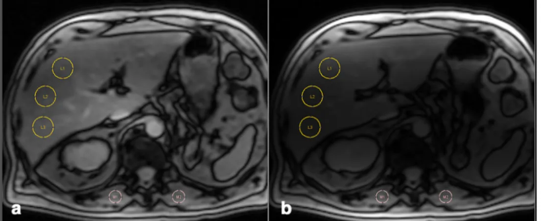
Imaging (SEDIA) proposed by Alustiza et al uses the same method with only 2 echoes (4 and 14 ms) and a different mathematical formula to calculate the LIC [21]. The results of the SEDIA’s model are better correlated with R2* and with LIC measured on liver biopsies [22]. In case of high iron overload, an add-in sequence using a shortest TE was pro-posed by Rose et al [21,23]. With SIR, it is important to only use the body coil, and no surface coils should be selected (especially those integrated in the patient’s bed) to avoid any signal gradient between the surface and the depth (Fig.3). This leads to a reduction of the signal-to-noise performance which ultimately limits the dynamic range of SIR and there-fore induces bias (due to the use of magnitude images). Another limitation of SIR is that the technique does not correct for fat, despite the fact that it uses“in-phase” echoes [24]. This can also lead to a relevant bias.
Which MRI technique is preferable?
For a long time, the R2* and SIR methods were opposed. They each have their limits.
The most significant advantages of SIR methods are their accessibility, being feasible on every machine in the world. With the improvement of ME-GRE sequences, SIR method is now considered less precise than R2* relaxometry for low or moderate iron overload. It can strongly overestimate the result if the measurements are made, by mistake, on images acquired with a surface coil.
The R2* method presents a risk for major underestimation of the overload if the signal is already collapsed at the first echo. This can be avoided at 1.5 T, in most cases, by setting a first very short echo, less than 1 ms, but this may be insuffi-cient in case of massive overload or even less on a 3-T device.
Fig. 3 SIR method applied correctly on an image (a) acquired with the body coil providing a normal liver to muscle ratio of 0.97. The wrong application is shown in image (b) on the same patient acquired using surface coil with a liver to muscle ratio of 0.43. This may lead to a
crucial mistake with the erroneous assumption that there is a significant iron overload. This is caused by the signal increase of the body parts closest to the surface coil
Fig. 2 Three examples (a–c) of a liver ME-GRE sequence obtained at 1.5 T with 12 echoes showing for each patient a selection of TE = 4.8 and 14.8 ms images (first line) and also a MRQuantif graph (second line) plotting the signal intensity according to TEs (signal of liver is yellow, signal of muscle in light red). a Patient without iron overload (LIC 12μmol/g). Visually, the liver signal is close to that of the paraspinous muscles on both echoes. On the graph, curve of the liver signal (yellow line) decreased progressively but stayed above that of the muscle (light
red line). The slight sinusoidal ripple of the signal according to the phase corresponded to a mild degree of fatty infiltration. b Mild iron overload (LIC 93 μmol/g). Visually, the liver signal is below that of the paraspinous muscles, particularly on the long TE. On the graph, the liver signal decreased more rapidly than that of the muscle. c Major iron over-load (LIC 355μmol/g). Visually, the liver signal is collapsed on both echoes. On the graph, the liver signal decreased very rapidly and reached the level of the background noise at the fourth echo (4.8 ms)
In this case, the use of the body coil makes it possible to compare with the muscle and to provide a ratio correcting the calculation error of the R2*. Indeed, the R2* and SIR methods can be carried out jointly from a single sequence if the body coil is selected, which is helpful in case of high overload and at 3 T [25].
Whenever the decision on the appropriate MRI method is made, keep the same method in case of patient follow-up. This is especially important for therapy monitoring as these methods (like R2 and R2*) should not be used interchange-ably in the same patient [26,27].
The following paragraphs are now based on R2* as the method of choice but you should keep in mind its limitations, at 3 T and in case of high overload.
Which MR protocol do I need for R2*?
Multi-echo gradient-echo (ME-GRE) sequences are means of choice to determine the R2*. As was done in early work on the R2* calculation, an ME-GRE sequence can be replaced by several GRE sequences with a single TE variation, but with the condition of not recalibrating between acquisitions [12].
The first echo time (TE) is the key parameter and should be chosen as short as possible, i.e., 1 ms or less [16,28–30]. Because the effect on the signal decrease is proportional to the magnetic field, at 3 T, to get the same level of result, the TE values should be divided by 2. This explains the limitation of quantifying high LIC at that field because it is difficult, at least routinely, to obtain the first TE below 0.5 ms. Furthermore, an appropriate number of echoes with short echo spacing (around 1 ms) should be used, and in literature, all calibrated sequences never had less than 8 echoes and we suggest at least 12 echoes. The TR is usually being set be-tween 25 and 120 ms with a low flip angle, which is important if the same sequence is also used to quantify fat.
The use of fat saturation can lead to systematically lower R2* values [31, 32]. This effect is significant for R2* > 300 s−1(when fat and water peaks begin to overlap) and therefore not relevant in patients with hereditary hemochro-matosis (HH) or dysmetabolic iron overload syndrome (DIOS) with expected R2* values far below this threshold. It has been shown that the spectral complexity of the fat signal introduces errors in R2* quantification in the presence of high fat concentration [33]. Using multi-peak modeling can miti-gate those effects on R2* measurements. Applying the fat saturation on the sequence used seems to be a possible solu-tion to this; however, most of the existing R2*-LIC biopsy calibrations have been mainly derived in the absence of fat suppression [34]. Moreover, joint quantification of steatosis could be necessary in a context of metabolic syndrome. Therefore, we advise to not use fat suppression for routine work to simplify the approach.
A single transverse slice through the liver (at the same time through the spleen) is traditionally acquired in clinical prac-tice, with only one breath-hold. All measurements should be performed prior to any administration of intravenous gadolin-ium chelate because this can change the clinically relevant results, especially with hepatocyte-specific contrast agents [35].
How do I measure the R2*?
R2* is usually reported in sec−1(s−1) in which T2* is simply its reciprocal (i.e., R2* = 1000/T2*, T2* is reported in ms). T2* can easily be converted by applying the factor of 1000, e.g., a T2* of 14 ms corresponds to 71.4 s−1(1000/14 = 71.4). We suggest using R2* rather than T2* in your report, because R2* is directly proportional, rather than inversely, to iron.
An important part is the application of the fitting algorithm on the average signal intensity at various echo times. The following decay models are available: mono (single) exponen-tials with/without truncation or with constant or variable off-set, complex or simple fitting, basic, baseline subtraction, sub-traction of measured image noise; bi-exponential [36]. These data-fitting procedures need correcting for confounding ef-fects, in particular image noise and signal modulations from fat. It is not yet clear which model appears to be the best, but the truncated model seems to be very accurate and the con-stant offset model very robust even for high iron levels [30]. The complex fit has been postulated as the best approach to avoid noise-related biases [37]. Nevertheless, as this is not a solution for daily clinical practice, we suggest that you adhere to two important aspects: decide on a decay model and stay with it, especially at follow-up examinations.
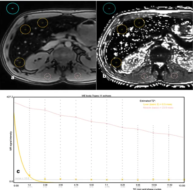
Freely available software is available in which the group from Rennes recently launched, MRQuantif (http://mrquantif.org). This DICOM-dedicated solution automatically selects the best method and the preferable algorithm depending on the data provided but gives also the opportunity to select a fitting method and visualize the matching of curve to the data points (Fig.4). This tool has the advantage to warn in case of incorrect or insufficient data. There are also other free tools building T2* maps, such as MRmap (https://sourceforge.net/projects/mrmap) or processing data allowing T2* calculation such as IronCalculator (http://www.ironcalculator.com) [38, 39]. We have to mention that all these free tools have no CE c e r t i f i c a t i o n a t t h e m o m e n t . T h e C M R t o o l s (Cardiovascular Imaging Solutions, London, UK) provide a paid alternative. MRI vendors also propose dedicated tools like StarMap from General Electric or MapIt from Siemens Healthineers.
MR vendors are proposing optional 2D or 3D multi-echo Dixon solutions integrating data processing, taking
also fat influence into account. With General Electric, the product is called “IDEAL-IQ”, with Philips “StarQuant” (or mDixon-Quant), and with Siemens Healthineers “LiverLab” (or qDixon). They produce T2* or R2* but also fat fraction maps by doing a pixelwise fitting. An advantage that results from this is the possibility of cal-culating the proton density fat fraction. Some of these
sequences have already been evaluated in literature with promising results at 1.5 T [40]. Comparison between 3D multi-echo Dixon approaches and the conventional, already-approved 2D GRE technique has shown excellent correlation [41]. Nevertheless, studies have shown some outliners or individual limitations such as reconstruction errors with fat-water swap. The first TE should be short Fig. 4 Example of a MR
evaluation using the MRQuantif software. Selected ROIs are placed manually, three in the liver, one in the spleen, two in paraspinal muscles, and one in the background noise (a). The software then automatically calculates R2* (and T2*) values and further provides results calculated with the selected SIR method (b). The LIC is then stated for each method. It also allows the user to choose between different calibration formulas and fitting procedures (c)
enough to provide correct R2* evaluation (and conse-quently fat fraction) and to avoid a major LIC underesti-mation in case of high overload, particularly at 3 T (Fig.5). We strongly recommend to first check that there is some liver signal left on the first two echoes of the native images before using the R2* map values.
The different approaches for placement of regions of inter-est (ROIs) or automatic whole-liver evaluation play a minor role in daily routine, and its pros and cons are negligible whereas whole-liver approaches are becoming favored in re-cent literature [42–45]. In general, several ROIs (2–3) should
be drawn with 2–3 cm2
, as large as possible [44]. Care should be taken to avoid large vessels or lesions [45]. Review the R2*
images for iron heterogeneity and avoid measuring only in these areas due to the possibility of sampling errors.
How to obtain the liver iron concentration
from the R2*?
This is probably one of the most important steps. Again, the golden rule is to mention that you must stay with your method, especially when it comes to monitoring of therapy. In contrast to the MR-based determination of fat, the MR quantification of iron is not a direct method; it is based on calibration with
Fig. 5 High LIC with 3-T imaging. a 2D ME-GRE sequence (first TE = 1.2 ms) obtained with body coil showing signal collapsed with a LIC of 521μmol Fe/g as estimated by SIR method. In the same patient, pixelwise R2* map built by the 3D ME-GRE vendor solution (b), performed with surface coil, provides a wrong mean R2* of 188 s−1 which corresponds to slight iron overload (LIC = 59μmol/g). The same
patient was also scanned with another 3-T system from a different vendor (picture not provided) giving even a lower wrong R2* estimation by the 3D ME-GRE pixelwise map. R2* calculated using the same ROIs by MRQuantif (c) providing selected truncation fitting, excluding most of the points, was 1587s−1corresponding to a LIC of 496μmol Fe/g
biopsy. Therefore, we need a formula to translate the R2* into the LIC.
1.5 Tesla
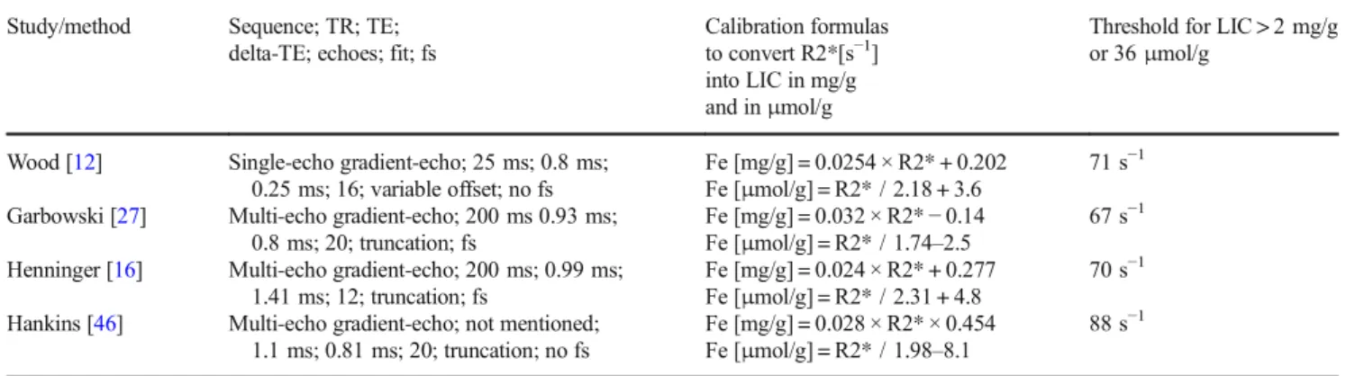
The group by Wood et al was one of the first to report such a calibration-based formula (Fe in mg/g dry weight [R2*] = 0.0254 × R2* + 0.202) [12]. Other groups also performed such studies, and differences were as mentioned in sequence parameters as well as in post-processing [27,46]. To transfer the R2* into the LIC, simply apply the measured R2* values to a calibration formula. Still, the question arises which cali-bration you should use? This depends on the sequence param-eters you have chosen and then the applied fit. Next, choose the validated formula from Table1below. The LIC is reported either in mg Fe/g or μmol Fe/g dry liver tissue; a con-version of mg/g in μmol/g is done by a multiplication by the factor 18 (Fe[μmol/g] = 18 × Fe[mg/g]), i.e., in detail 1 μmol~55.845 μg (=atomic weight of iron).
The problem is that all available calibration formulas differ from each other, but why is this so? Firstly, all sequences have different acquisition parameters and post-processing fitting algorithms. Further differences in post-biopsy sample process-ing may also explain the difference between the calibration curves in literature [27]. These are the two major points. Nevertheless, it was shown that pooled data from studies that have a low initial TE in common provide relatively similar calibration results [16]. In general, when taking the studies by Wood, Garbowski, Hankins, and Henninger into account, a R2* threshold of 70 s−1 is in general a good surrogate and first orientation [12,16,27,46]. Nevertheless, the studies by Kühn et al provide distinct different R2* thresholds [33,47]. The reason can be seen in the histological evaluation of the liver biopsy samples (done by a subjective grading with no quantitative LIC determination), performing the MRI after the liver biopsy and the imaging parameters with a relatively low initial TE of 2.4 and only 3 acquired echoes, all based on a
3-point Dixon technique. Therefore, we must be aware when comparing different techniques and calibration with each oth-er. Nevertheless, sequence parameters provided in Table2are a good orientation, rough deviations of which should be avoided.
With the other abdominal organs (pancreas and spleen), there is no calibration that translates the R2* value into any quantitative unit for tissue iron but the same R2* technique as for the liver can be used. Pancreas and spleen R2* measure-ments can readily be obtained using the same approach as for liver R2*; they “come for free”. Schwenzer et al measured R2* of the liver, spleen, and pancreas in a healthy population, to get an idea of possible threshold [48]. They used a 12-echo gradient-echo sequence with fat saturation (first TE 2.6 ms), mono-exponential decay. The R2* range for the liver was 21.8–73.5 s−1(n = 129 patients; R2* mean 35.6) which is also
compatible with most studies. For the pancreas, the range was 15.4–38.6 s−1(n = 61 patients; R2* mean 24.1) and for the
spleen, 8.8–69 s−1(n = 129 patients; R2* mean 22.8). A pan-creas R2* of 100 s−1appears to represent a risk threshold for predicting cardiac iron overload with a“clean” pancreas pro-viding a nearly 100% negative predictive value for cardiac iron deposition [49]. For the spleen, 70 s−1can be chosen as a reliable threshold, whereat 100 s−1is a pathologic condition. R2* measurements of the pancreas and the spleen offer valu-able information in the management of patients with hyperferritinemia [50].
3 Tesla
For the moment, there is only one reference analyzing the SIR and R2* methods in comparison with the LIC obtained by biopsy in a significant number of patients [25]. The conver-sion formula proposed from R2* calculated after subtraction of the background noise is LIC (μmol) = 0.314 R2* − 0.96. We could simplify in LIC (μmol) = R2* / 3.2. The increased sensitivity at 3 T allows for more precise analysis and Table 1 LIC calibration formulas at 1.5 T and R2* thresholds from literature
Study/method Sequence; TR; TE; delta-TE; echoes; fit; fs
Calibration formulas to convert R2*[s−1] into LIC in mg/g and inμmol/g
Threshold for LIC > 2 mg/g or 36μmol/g
Wood [12] Single-echo gradient-echo; 25 ms; 0.8 ms; 0.25 ms; 16; variable offset; no fs
Fe [mg/g] = 0.0254 × R2* + 0.202 Fe [μmol/g] = R2* / 2.18 + 3.6
71 s−1 Garbowski [27] Multi-echo gradient-echo; 200 ms 0.93 ms;
0.8 ms; 20; truncation; fs
Fe [mg/g] = 0.032 × R2*− 0.14 Fe [μmol/g] = R2* / 1.74–2.5
67 s−1 Henninger [16] Multi-echo gradient-echo; 200 ms; 0.99 ms;
1.41 ms; 12; truncation; fs
Fe [mg/g] = 0.024 × R2* + 0.277
Fe [μmol/g] = R2* / 2.31 + 4.8 70 s
−1
Hankins [46] Multi-echo gradient-echo; not mentioned; 1.1 ms; 0.81 ms; 20; truncation; no fs
Fe [mg/g] = 0.028 × R2* × 0.454
Fe [μmol/g] = R2* / 1.98–8.1 88 s
−1
detection of mild iron overload; conversely, it can be difficult to quantify severe iron overload beyond 150μmol/g, unless the body coil is used to combine the two methods.
A complete checklist for the whole procedure is provided in Table3.
How to report?
The cut-off value for pathological LIC and hence iron over-load has been defined as 36μmol Fe/g or 2 mg Fe/g of dry
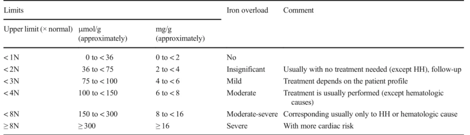
weight [21]. The LIC should be calculated and reported; a simple R2* value of the liver does not help any clinician to get an idea of what is going on—calibration is the key [51]. It is important to speak one common language and the LIC is well known among clinicians. There is a terminology pro-posed in 2000 by EASL but a more detailed version taking in account more recent knowledge can be proposed (Table4) [1].
The distinction between the different iron distribution pat-terns is an important aspect in the differential diagnosis of iron overload disorders; therefore, R2* of the spleen and the pan-creas should also be reported and, if possible, evaluated as pathological or not [52].
In therapy monitoring, the baseline finding and the calculated LIC should be mentioned, if available. An example of monitoring a patient under chelation with MRI is provided in Fig. 6. We strongly suggested struc-tured reporting. The software MRQuantif, proposed by the Rennes team, automatically builds a report and stores a data file.
Closing comments
We are aware that in literature, concerning R2* relaxometry, there is strong doubt on its reproducibility with the fear that recalibration is necessary for any mod-ifications on sequence parameters and post-processing. This “fear” is partly justified, of course, especially if you want to have a very accurate quantification. Measured R2* values depend an awful lot on how the images are processed. While these effects are relatively modest at LIC levels typically found in HH, they can become significant at higher LIC’s. It could be shown that changing sequence parameters and post-processing alters results but not to the expected extent [16–18].
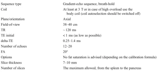
Table 2 Sequence parameters for
R2* Sequence type Gradient-echo sequence, breath-hold
Coil At least at 3 T or in case of high overload use the
body coil (coil autoselection should be switched off)
Plane/orientation Axial
Field-of-view 38–40 cm
TR ~ 120 ms
TE initial < 1 ms (as low as possible)
delta-TE 0.25–1.4 ms
Number of echoes 12–20
FA 20°
Options No fat saturation is advised (depending on the calibration formula)
Slice thickness 7–10 mm
Number of slices The maximum allowed, from the spleen to the pancreas
Table 3 Checklist for LIC evaluation SIR methods
• You could use several single-echo GRE but preferably ME-GRE to reduce the acquisition time, to be able to combine both methods and to quantify fat.
• For Rennes algorithm (for both 1.5-T and 3-T systems), use the pro-tocol described on thehttps://imagemed.univ-rennes1.
fr/en/mrquantif/protocols.phpweb page. For SEDIA protocol at 1.5 T,
global parameters are identical but only the two echoes at 4 and 14 ms TEs are used.
• Use only body coil!
• To get LIC preferably, use the DICOM software MRQuantif to have a control of the coil selected or go on-line tomrquantif.orgorwww. sedia.es
R2* methods
• Use a 2D ME-GRE sequence (or several single-echo GRE if not available) and/or a vendor 3D ME-GRE optional sequence. • Check that the first echo is about 1 ms or even less.
• Prefer a 2D ME-GRE sequence using body coil as described on the
https://imagemed.univ-rennes1.fr/mrquantif/protocolsif you are using
a 3 T or dealing with highly overloaded patients
• If you use a 2D ME-GRE sequence, choose your software option and the appropriate fit
• Check that the R2* calculated is coherent with the liver signal • Select your R2* to LIC conversion formula
• Mention the LIC and R2* values of spleen/pancreas in your report, define the thresholds for the clinicians
The goal is to have a tool that can allow for different ac-quisition parameters, determine the best method of analysis, and provide an LIC value that is sufficiently reproducible whatever the brand of the device or even the magnetic field
used. Until this type of software is scientifically validated, it is important that you choose your method, decide for the cali-bration formula that fits most to your settings, and stay with that method.
Fig. 6 A 15-year old patient with secondary iron overload due to blood transfusion therapy. R2* with“in-house” ME-GRE sequences revealed a pathologic value of 162 s−1(a), confirmed by qDixon (LiverLab) (b) with 169 s−1. After 2 years of chelation therapy, the values normalized to 35 s−1
(ME-GRE) (c)/32 s−1(qDixon) (d). Further iron overload of the spleen was initially detected (R2* 102 s−1). Spleen values also decreased to a normal value under therapy (R2* 21 s−1)
Table 4 Proposition of a classification of iron overload severity
Limits Iron overload Comment
Upper limit (× normal) μmol/g (approximately)
mg/g
(approximately)
< 1N 0 to < 36 0 to < 2 No
< 2N 36 to < 75 2 to < 4 Insignificant Usually with no treatment needed (except HH), follow-up
< 3N 75 to < 100 4 to < 6 Mild Treatment depends on the patient profile
< 4N 100 to < 150 6 to < 8 Moderate Treatment is usually performed (except hematologic causes)
< 8N 150 to < 300 8 to < 16 Moderate-severe Corresponding usually only to HH or hematologic cause
Funding Information Open access funding provided by University of Innsbruck and Medical University of Innsbruck. The authors state that this work has not received any funding.
Compliance with ethical standards
Guarantor The scientific guarantor of this publication is PD Dr. Benjamin Henninger.
Conflict of interest The authors of this manuscript declare no relation-ships with any companies, whose products or services may be related to the subject matter of the article.
Statistics and biometry No complex statistical methods were necessary for this paper.
Informed consent Written informed consent was not required for this study because it is a review/special report.
Ethical approval Institutional Review Board approval was not required because it is a review/special report.
Methodology • review/special report
Open AccessThis article is distributed under the terms of the Creative C o m m o n s A t t r i b u t i o n 4 . 0 I n t e r n a t i o n a l L i c e n s e ( h t t p : / / creativecommons.org/licenses/by/4.0/), which permits unrestricted use, distribution, and reproduction in any medium, provided you give appro-priate credit to the original author(s) and the source, provide a link to the Creative Commons license, and indicate if changes were made.
References
1. European Association For The Study Of The L (2010) EASL clin-ical practice guidelines for HFE hemochromatosis. J Hepatol 53:3– 22
2. Hoffbrand AV, Taher A, Cappellini MD (2012) How I treat trans-fusional iron overload. Blood 120:3657–3669
3. Adams PC, Barton JC (2010) How I treat hemochromatosis. Blood 116:317–325
4. Golfeyz S, Lewis S, Weisberg IS (2018) Hemochromatosis: patho-physiology, evaluation, and management of hepatic iron overload with a focus on MRI. Expert Rev Gastroenterol Hepatol 12:767– 778
5. Ho PJ, Tay L, Lindeman R, Catley L, Bowden DK (2011) Australian guidelines for the assessment of iron overload and iron chelation in transfusion-dependent thalassaemia major, sickle cell disease and other congenital anaemias. Intern Med J 41:516–524 6. Angelucci E, Barosi G, Camaschella C et al (2008) Italian Society
of Hematology practice guidelines for the management of iron over load i n t hala ssemia maj or a nd rel ate d disorde rs. Haematologica 93:741–752
7. Lim RP, Tuvia K, Hajdu CH et al (2010) Quantification of hepatic iron deposition in patients with liver disease: comparison of chem-ical shift imaging with single-echo T2*-weighted imaging. AJR Am J Roentgenol 194:1288–1295
8. Queiroz-Andrade M, Blasbalg R, Ortega CD et al (2009) MR im-aging findings of iron overload. Radiographics 29:1575–1589 9. Schieda N, Ramanathan S, Ryan J, Khanna M, Virmani V, Avruch
L (2014) Diagnostic accuracy of dual-echo (in- and opposed-phase)
T1-weighted gradient recalled echo for detection and grading of hepatic iron using quantitative and visual assessment. Eur Radiol 24:1437–1445
10. Virtanen JM, Pudas TK, Ratilainen JA, Saunavaara JP, Komu ME, Parkkola RK (2012) Iron overload: accuracy of in-phase and out-of-phase MRI as a quick method to evaluate liver iron load in haema-tological malignancies and chronic liver disease. Br J Radiol 85: e162–e167
11. St Pierre TG, Clark PR, Chua-anusorn W et al (2005) Noninvasive measurement and imaging of liver iron concentrations using proton magnetic resonance. Blood 105:855–861
12. Wood JC, Enriquez C, Ghugre N et al (2005) MRI R2 and R2* mapping accurately estimates hepatic iron concentration in transfusion-dependent thalassemia and sickle cell disease patients. Blood 106:1460–1465
13. Westwood MA, Anderson LJ, Firmin DN et al (2003) Interscanner reproducibility of cardiovascular magnetic resonance T2* measure-ments of tissue iron in thalassemia. J Magn Reson Imaging 18:616– 620
14. Kirk P, He T, Anderson LJ et al (2010) International reproducibility of single breathhold T2* MR for cardiac and liver iron assessment among five thalassemia centers. J Magn Reson Imaging 32:315– 319
15. Hernando D, Levin YS, Sirlin CB, Reeder SB (2014) Quantification of liver iron with MRI: state of the art and remaining challenges. J Magn Reson Imaging.https://doi.org/10.1002/jmri. 24584
16. Henninger B, Zoller H, Rauch S et al (2015) R2* relaxometry for the quantification of hepatic iron overload: biopsy-based calibration and comparison with the literature. Rofo 187:472–479
17. Meloni A, Rienhoff HY Jr, Jones A, Pepe A, Lombardi M, Wood JC (2013) The use of appropriate calibration curves corrects for systematic differences in liver R2* values measured using different software packages. Br J Haematol 161:888–891
18. Tanner MA, He T, Westwood MA, Firmin DN, Pennell DJ (2006) Multi-center validation of the transferability of the magnetic reso-nance T2* technique for the quantification of tissue iron. Haematologica 91:1388–1391
19. Serai SD, Fleck RJ, Quinn CT, Zhang B, Podberesky DJ (2015) Retrospective comparison of gradient recalled echo R2* and spin-echo R2 magnetic resonance analysis methods for estimating liver iron content in children and adolescents. Pediatr Radiol 45:1629– 1634
20. Gandon Y, Olivie D, Guyader D et al (2004) Non-invasive assess-ment of hepatic iron stores by MRI. Lancet 363:357–362 21. Alustiza JM, Artetxe J, Castiella A et al (2004) MR quantification
of hepatic iron concentration. Radiology 230:479–484
22. Castiella A, Alustiza JM, Emparanza JI, Zapata EM, Costero B, Diez MI (2011) Liver iron concentration quantification by MRI: are recommended protocols accurate enough for clinical practice? Eur Radiol 21:137–141
23. Rose C, Vandevenne P, Bourgeois E, Cambier N, Ernst O (2006) Liver iron content assessment by routine and simple magnetic res-onance imaging procedure in highly transfused patients. Eur J Haematol 77:145–149
24. Hernando D, Kuhn JP, Mensel B et al (2013) R2* estimation using “in-phase” echoes in the presence of fat: the effects of complex spectrum of fat. J Magn Reson Imaging 37:717–726
25. d’Assignies G, Paisant A, Bardou-Jacquet E et al (2018) Non-invasive measurement of liver iron concentration using 3-Tesla magnetic resonance imaging: validation against biopsy. Eur Radiol 28:2022–2030
26. Wood JC, Zhang P, Rienhoff H, Abi-Saab W, Neufeld E (2014) R2 and R2* are equally effective in evaluating chronic response to iron chelation. Am J Hematol 89:505–508
27. Garbowski MW, Carpenter JP, Smith G et al (2014) Biopsy-based calibration of T2* magnetic resonance for estimation of liver iron concentration and comparison with R2 Ferriscan. J Cardiovasc Magn Reson 16:40
28. Alustiza Echeverria JM, Castiella A, Emparanza JI (2012) Quantification of iron concentration in the liver by MRI. Insights Imaging 3:173–180
29. Ghugre NR, Enriquez CM, Coates TD, Nelson MD Jr, Wood JC (2006) Improved R2* measurements in myocardial iron overload. J Magn Reson Imaging 23:9–16
30. Beaumont M, Odame I, Babyn PS, Vidarsson L, Kirby-Allen M, Cheng HL (2009) Accurate liver T2 measurement of iron overload: a simulations investigation and in vivo study. J Magn Reson Imaging 30:313–320
31. Meloni A, Tyszka JM, Pepe A, Wood JC (2015) Effect of inversion recovery fat suppression on hepatic R2* quantitation in transfusion-al siderosis. AJR Am J Roentgenol 204:625–629
32. Sanches-Rocha L, Serpa B, Figueiredo E, Hamerschlak N, Baroni R (2013) Comparison between multi-echo T2* with and without fat saturation pulse for quantification of liver iron overload. Magn Reson Imaging 31:1704–1708
33. Kuhn JP, Hernando D, Munoz del Rio A et al (2012) Effect of multipeak spectral modeling of fat for liver iron and fat quantifica-tion: correlation of biopsy with MR imaging results. Radiology 265:133–142
34. Krafft AJ, Loeffler RB, Song R et al (2016) Does fat suppression via chemically selective saturation affect R2*-MRI for transfusional iron overload assessment? A clinical evaluation at 1.5T and 3T. Magn Reson Med 76:591–601
35. Hernando D, Wells SA, Vigen KK, Reeder SB (2015) Effect of hepatocyte-specific gadolinium-based contrast agents on hepatic fat-fraction and R2(). Magn Reson Imaging 33:43–50
36. Sirlin CB, Reeder SB (2010) Magnetic resonance imaging quanti-fication of liver iron. Magn Reson Imaging Clin N Am 18(359– 381):ix
37. Hernando D, Kramer JH, Reeder SB (2013) Multipeak fat-corrected complex R2* relaxometry: theory, optimization, and clin-ical validation. Magn Reson Med 70:1319–1331
38. Git KA, Fioravante LA, Fernandes JL (2015) An online open-source tool for automated quantification of liver and myocardial iron concentrations by T2* magnetic resonance imaging. Br J Radiol 88:20150269
39. Messroghli DR, Rudolph A, Abdel-Aty H et al (2010) An open-source software tool for the generation of relaxation time maps in magnetic resonance imaging. BMC Med Imaging 10:16
40. Henninger B, Zoller H, Kannengiesser S, Zhong X, Jaschke W, Kremser C (2017) 3D multiecho Dixon for the evaluation of hepatic iron and fat in a clinical setting. J Magn Reson Imaging 46:793–800 41. Serai SD, Smith EA, Trout AT, Dillman JR (2018) Agreement be-tween manual relaxometry and semi-automated scanner-based multi-echo Dixon technique for measuring liver T2* in a pediatric and young adult population. Pediatr Radiol 48:94–100
42. Positano V, Salani B, Pepe A et al (2009) Improved T2* assessment in liver iron overload by magnetic resonance imaging. Magn Reson Imaging 27:188–197
43. McCarville MB, Hillenbrand CM, Loeffler RB et al (2010) Comparison of whole liver and small region-of-interest measure-ments of MRI liver R2* in children with iron overload. Pediatr Radiol 40:1360–1367
44. Campo CA, Hernando D, Schubert T, Bookwalter CA, Pay AJV, Reeder SB (2017) Standardized approach for ROI-based measure-ments of proton density fat fraction and R2* in the liver. AJR Am J Roentgenol 209:592–603
45. Meloni A, Luciani A, Positano V et al (2011) Single region of interest versus multislice T2* MRI approach for the quantification of hepatic iron overload. J Magn Reson Imaging 33:348–355 46. Hankins JS, McCarville MB, Loeffler RB et al (2009) R2*
mag-netic resonance imaging of the liver in patients with iron overload. Blood 113:4853–4855
47. Kuhn JP, Meffert P, Heske C et al (2017) Prevalence of fatty liver disease and hepatic Iron overload in a Northeastern German popu-lation by using quantitative MR imaging. Radiology 284:706–716 48. Schwenzer NF, Machann J, Haap MM et al (2008) T2* relaxometry in liver, pancreas, and spleen in a healthy cohort of one hundred twenty-nine subjects-correlation with age, gender, and serum ferri-tin. Invest Radiol 43:854–860
49. Wood JC (2014) Use of magnetic resonance imaging to monitor iron overload. Hematol Oncol Clin North Am 28(747–764):vii 50. Zoller H, Henninger B (2016) Pathogenesis, diagnosis and
treat-ment of hemochromatosis. Dig Dis 34:364–373
51. Bacigalupo L, Paparo F, Zefiro D et al (2016) Comparison between different software programs and post-processing techniques for the MRI quantification of liver iron concentration in thalassemia pa-tients. Radiol Med 121:751–762
52. Franca M, Marti-Bonmati L, Porto G et al (2018) Tissue iron quan-tification in chronic liver diseases using MRI shows a relationship between iron accumulation in liver, spleen, and bone marrow. Clin Radiol 73:215 e211–215 e219
Publisher’s note Springer Nature remains neutral with regard to jurisdictional claims in published maps and institutional affiliations.