The theory of calculi with explicit substitutions revisited

HAL Id: hal-00111285

https://hal.archives-ouvertes.fr/hal-00111285v3

Preprint submitted on 17 Jan 2007

HAL is a multi-disciplinary open access

archive for the deposit and dissemination of

sci-entific research documents, whether they are

pub-lished or not. The documents may come from

L’archive ouverte pluridisciplinaire HAL, est

destinée au dépôt et à la diffusion de documents

scientifiques de niveau recherche, publiés ou non,

émanant des établissements d’enseignement et de

The theory of calculi with explicit substitutions revisited

Delia Kesner

To cite this version:

The theory of calculi with explicit substitutions

revisited

Delia Kesner

October 9, 2006

Abstract

Calculi with explicit substitutions are widely used in different areas of com-puter science such as functional and logic programming, proof-theory, theorem proving, concurrency, object-oriented languages, etc. Complex systems with ex-plicit substitutions were developed these last 15 years in order to capture the good computational behaviour of the original system (with meta-level substitutions) they were implementing.

In this paper we first survey previous work in the domain by pointing out the motivations and challenges that guided the developement of such calculi. Then we use very simple technology to establish a general theory of explicit substitutions for the lambda-calculus which enjoys all the expected properties such as simulation of one-step beta-reduction, confluence on meta-terms, preservation of beta-strong normalisation, strong normalisation of typed terms and full composition. Also, the calculus we introduce turns out to admit a natural translation into Linear Logic’s proof-nets.

Contents

1 Introduction 3

2 Syntax 8

3 Confluence on metaterms 11

3.1 Confluence by simultaneous reduction . . . 13

3.2 Confluence by interpretation . . . 19

3.2.1 A calculus with simultaneous substitution . . . 19

3.2.2 A calculus with normal simultaneous substitutions . . . 21

3.2.3 Relatingλes and λnss . . . 22

3.2.4 Relatingλnss and λes . . . 23

4 Preservation ofβ-strong normalisation 24 4.1 Theλesw-calculus . . . 25

4.2 Relatingλes and λesw . . . 28

4.3 TheΛI-calculus . . . 28

4.4 Relatingλesw and ΛI . . . 29

4.5 Solving the puzzle . . . 30

5 Recovering the untypedλ-calculus 31 5.1 Fromλ-calculus to λes-calculus . . . 32

5.2 Fromλes-calculus to λ-calculus . . . 32

6 The typedλes-calculus 33 6.1 Typing Rules . . . 33

6.2 Subject Reduction . . . 34

7 Recovering the typedλ-calculus 34 8 Strong normalisation of typedλes-terms 35 8.1 Linear Logic’s proof-nets . . . 35

8.2 Fromλes-terms to Proof-nets . . . 39

8.3 Discussion . . . 51

9 PSN implies SN 52

10 Conclusion 52

1

Introduction

This paper is about explicit substitutions (ES), an intermediate formalism that - by decomposing theβ rule into more atomic steps - allows a better understanding of the

execution models ofλ-calculus.

We first survey previous work in the domain, by pointing out the motivations that were guided the developement of such calculi as well as the main challenge behind their formulations. The goal of our work is to move back to previous works and results in the domain in order to establish a general and simple theory of explicit substitutions being able to capture all of them by using very simple technology.

Explicit substitutions

Inλ-calculus, the evaluation process is modelled by β-reduction and the replacement of

formal parameters by its corresponding arguments is modelled by substitution. While substitution inλ-calculus is a meta-level operation described outside the calculus

it-self, in calculi with ES it is internalised and handled by symbols and reduction rules belonging to the proper syntax of the calculus. However the two formalisms are still very close: lets{x/u} denote the result of substituting all the free occurrences of x in s by u, then one defines β-reduction as

(λx.s) v →βs{x/v}

where the operations{x/v} can be defined modulo α-conversion1_{by induction on}

s as follows:

x{x/v} := v

y{x/v} := y ifx 6= y (t u){x/v} := (t{x/v} u{x/v})

(λy.t){x/v} := λy.(t{x/v}) ifx 6= y and y 6∈ fv(v)

Then, the simplest way to specify aλ-calculus with explicit substitution is to

ex-plicitly encode the previous definition, so that one still works moduloα-conversion,

yielding the calculus known asλx which is shown in Figure 1.

(λx.t) v → t[x/v] x[x/v] → v

x[y/v] → x ifx 6= y (t u)[x/v] → (t[x/v] u[x/v])

(λx.t)[y/v] → λx.(t[y/v]) ifx 6= y and x 6∈ fv(v)

Figure 1: Reduction rules for theλx-calculus

1_{Definition of substitution moduloα-conversion avoids to explicitly deal with the variable capture case}

This reduction system corresponds to the minimal behaviour that can be found in most of the well-known calculi with ES appearing in the literature: substitutions are incorporated into the language and manipulated explicitly,β-reduction is implemented

in two stages, first by the application of the first rule, which activates the calculus of substitutions, then by propagation of the substitution until variables are reached. More sophisticated treatment of substitutions considers also a composition operator allowing interactions between them.

Related Work

In these last years there has been a growing interest inλ-calculi with explicit

substitu-tions. They were defined in de Bruijn notation [ACCL91, HL89, Les94, KR95, Kes96, FKP96], or level notation [LRD95], or via combinators [GL99], or simply by named variables notation as shown above [Lin86, Lin92, Ros92, BR95].

An abstract presentation of such calculi can be found in [Kes96, Kes00], where a (syntactic) axiomatisation is used to define and study them.

In any case, all these calculi were all introduced as a bridge between the clas-sicalλ-calculus and concrete implementations of functional programming languages

such as CAML [Oca], SML [MTH90], Miranda [Tur85], Haskell [HPJP92] or proof-assistants such as Coq [Coq], PVS [PVS], HOL [HOL], LEGO [LEG], Maude [Mau] and ELAN [ELA].

Now, the implementation of the atomic substitution operation by several elementary explicit steps comes at a price. Indeed, whileλ-calculus is perfectly orthogonal2_, calculi with ES suffer at least from the well-known diverging example

t[y/v][x/u[y/v]]∗← ((λx.t) u)[y/v] →∗_t[x/u][y/v]

Different solutions were adopted by the calculi in the literature in order to close this diagram. If no new rewriting rules are added to those in Figure 1, then reduction turns out to be confluent on terms but not on metaterms3_{. If naive rules for composition are} also considered, then one recovers confluence on metaterms but paying an important price: there exist terms which are strongly normalisable inλ-calculus but not in the

corresponding explicit version of theλ-calculus. This phenomenon, known as Melli`es’

counter-example [Mel95], shows a flaw in the design of calculi with ES in that they are supposed to implement their underlying calculus (in our case theλ-calculus) without

losing its good properties. More precisely, let us callλZaλ-calculus with ES and let us consider a mapping toλfromλ-syntax to λZ-syntax (sometimes this mapping is just the identity). We identify the following list of properties:

(C) The refined reduction relationλZis confluent on terms: Ifu∗λZ← t → ∗

λZ v, then there ist′such thatu →∗λZt

′ ∗ λZ← v.

(MC) The refined reduction relationλZis confluent on metaterms.

2_{Does not have critical pairs.}

(PSN) The reduction relationλZpreservesβ-strong normalisaion: If t ∈ SNβ, then

toλ(t) ∈ SNλZ.

(SN) Strong normalisation holds forλZ-typed terms: Ift is typed, then t ∈ SNλZ.

(SIM) Any evaluation step inλ-calculus can be implemented by λZ: Ift →β t′, then

toλ(t) →∗λZtoλ(t ′_).

(FC) Full composition can be implemented byλZ:t[x/u] λZ-reduces tot{x/u} for an appropriate (and natural) notion of substitution onλZ-terms.

The result of Melli`es has revived the interest in ES since after his counterexample there was a clear challenge to find a calculus having all the good properties mentioned above.

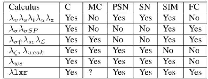
There are several propositions that give (sometimes partial) answers to this chal-lenge, they are summarised in Figure 2.

Calculus C MC PSN SN SIM FC

λυλsλtλuλx Yes No Yes Yes Yes No

λσλσSP Yes No No No Yes Yes

λσ⇑λseλL Yes Yes No No Yes Yes

λζ,λweak Yes Yes Yes Yes No No

λws Yes Yes Yes Yes Yes No

λlxr Yes ? Yes Yes Yes Yes Figure 2: Summarising previous work in the field

In other words, there are many ways to avoid Melli`es’ counter-example in order to recover the PSN property. One of them is to simply forbid the substitution oper-ators to cross lambda-abstractions [LM99, For02]; another consists of avoiding com-position of substitutions [BBLRD96]; another one imposes a simple strategy on the calculus with explicit substitutions to mimic exactly the calculus without explicit sub-stitutions [GL98]. The first solution leads to weak lambda calculi, not able to ex-press strong beta-equality, which is used for example in implementations of proof-assistants [Coq, HOL]. The second solution is drastic as composition of substitutions is needed in implementations of HO unification [DHK95] or functional abstract ma-chines [HMP96]. The last one exploits very little of the notion of explicit substitutions because they can be neither composed nor even delayed.

In order to cope with this problem David and Guillaume [DG01] defined a calculus with labels calledλws, which allows controlled composition of explicit substitutions without losing PSN and SN [DCKP00]. But theλws-calculus has a complicated syntax and its named version [DCKP00] is even less readable.

The strong normalisation proof forλwsgiven in [DCKP00] reveals a natural seman-tics for composition of explicit substitutions via Linear Logic’s proof-nets, suggesting that weakening (explicit erasure) and contraction (explicit duplication) can be added to the calculus without losing termination. These are the starting points of the ideas

proposed by theλlxr-calculus [KL05], which is in some sense a (complex) precursor

of theλes-calculus that we present in this work. Indeed, λ-terms can not be viewed

directly asλlxr-terms, so that we prefer to adopt λx-syntax for λes, thus avoiding

special encodings in order to explicitly incorporate weakening and contractions inside

λ-terms. Moreover, the reduction system of λlxr is defined via 6 equations and 19

rewriting rules, thus requiring an important amount of combinatory reasoning when showing its properties.

Another calculi with safe notions of compositions appear for example in [SFM03, Sak]. The first of them lacks full composition and confluence on metaterms. The sec-ond of them specifies commutation of independent substitutions by a rewriting rule (instead of an equation), thus leading to complicated notions and proofs of its under-lying normalisation properties. Here, we choose to make a minimal (just one) use of equational reasoning to axiomatise commutation of independent substitution. This will turn out to be essential to achieve the definition of a simple language being easy to un-derstand, which can be projected into another elementary system like proof-nets, and whose properties can be proved with simple and natural proof techniques.

Last but not least, confluence on metaterms of both calculi in [KL05] and [Sak] on metaterms is only conjectured but not yet proved.

The logical meaning of explicit substitutions

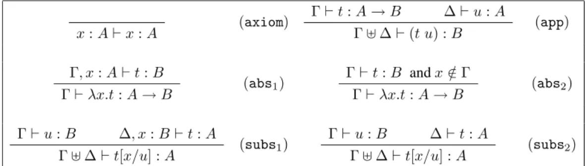
Cut elimination is a logical evaluation process allowing to relate explicit substitution to a more atomic process. Indeed, the cut elimination process can be interpreted as the elimination of explicit substitutions. For example, let us consider the following sequent proof:

D

Γ ⊢ A Γ, A ⊢ A (axiom) (cut) Γ ⊢ A

If we want to eliminate the last cut rule used in this proof, it is sufficient to take the proof

D Γ ⊢ A

which proves exactly the same sequentΓ ⊢ A but without the last cut rule. That is,

in the cut elimination process, the first proof reduces to the second one. Now, let us interpret proofs by terms and propositions by types as suggested by the Curry-Howard correspondence. We then get

Γ ⊢ v : A Γ, x : A ⊢ x : A (proj) (subs) Γ ⊢ x[x/v] : A

which suggests that the process of cut elimination consists in reducing the termx[x/v]

to the termv, exactly as in the Var rule of the calculus λx written as (Var) x[x/v] → v

These remarks put in evidence the fact that explicit substitution is a term nota-tion for the cut rule, and that reducnota-tion rules for explicit substitunota-tions behave like cut elimination rules. However,λ and λx basic (typed) syntax are taken from a

natu-ral deduction logical system, where application annotates implication elimination and abstraction annotates implication introduction. That means thatλx (typed) syntax is

based on a logical system mixing natural deduction with sequent calculus such that the meta-level operation in the normalisation process is replaced by a more elementary concept of cut elimination.

It is worth noticing that one can either define an explicit substitution calculus inter-preting cut-elimination, in such a way to have a perfect Curry-Howard correspondence between them, as is done by Hugo Herbelin in [Her94]: there terms encode proofs, types encode propositions and reduction encodes cut-elimination in intuitionistic quent calculus. So that the ideas we present in this paper can also be adapted to se-quent calculus notation. We refer the reader to [Len06] for a systematic study of cut elimination in intuitionistic sequent calculus via proof-terms.

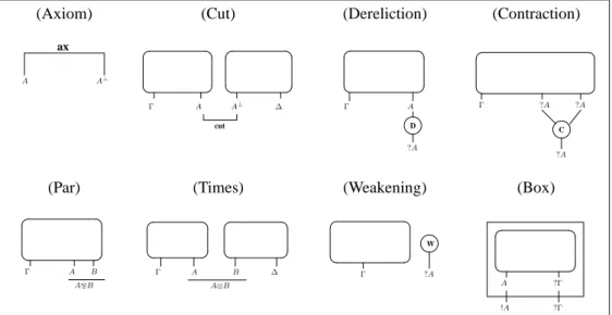
Linear logic and proof-nets

Linear Logic decomposes the intuitionistic logical connectives, like the implication, into more atomic, resource-aware connectives, like the linear implication and the ex-plicit erasure and duplication operators given by the exponentials which provide a more refined computational model that the one given by theλ-calculus. However, sequent

presentations of Linear Logic can contain a lot of details that are uninteresting (or bu-reaucratic). The main idea of proof-nets is to solve this problem by providing a sort of representative of an equivalence class of proofs in the sequent calculus style that differ only by the order of application of some logical or structural rules. Cut elimina-tion over proof-nets is then a kind of normalisaelimina-tion procedure over these equivalence classes. Using different translations of theλ-calculus into Proof Nets, new abstract

machines have been proposed, exploiting the Geometry of Interaction [Gir89, AJ92], culminating in the works on optimal reduction [GAL92, Lam90].

Some calculi with explicit substitutions [DCKP03, KL05] have been already put in relation with natural extended notions of proof-nets. In particular, one defines a typed version of the calculus and shows how to translate it into Proof Nets and how to estab-lish, using this translation, a simulation of the reduction rules for explicit substitutions via cut elimination in Proof Nets. As an immediate consequence of this simulation, one proves that a simply typed version of the calculus is strongly normalizing. An im-portant property of the simulation is that each step in the calculus with ES is simulated by a constant number of steps in proof-nets: this shows that the two systems are very close, unlike what happens when simulating theλ-calculus. This gives also a powerful

tool to reason about the complexity ofβ-reduction.

We apply this idea to theλes-calculus that we introduce in this paper so that we

obtain strong normalisation for typedλes-terms via simulation of reduction in

Summary

We present a calculus with ES using the named variable presentation, which makes some essential properties of explicit substitutions more apparent, by abstracting out the details of renaming and updating of de Bruijn notation. The main ideas and results of the paper can be summarised by the following points:

• Named variable notation and concise/simple syntax is used to define a calculus

with explicit substitutions calledλes. There is no use of explicit contraction or

weakening.

• The calculus enjoys simulation of one-step β-reduction, confluence on metaterms

(and thus on terms), preservation ofβ-strong normalisation, strong normalisation

of typed terms and implementation of full composition.

• We establish connections with untyped λ-calculus and typed λ-calculus. • We give a natural translation into Linear Logic’s proof-nets.

• We give some ideas for future work and applications.

The rest of the paper is organised as follows. Section 2 introduces syntax for

λes-terms as well as appropriate notions of equivalence and reduction. We show there some fundamental properties of the calculus such as full composition and termination of the substitution calculus alone. In Section 3 we develop a proof of confluence for metaterms. This proof uses an interpretation method based on the confluence property of a simpler calculus that we define in the same section. Preservation of β-strong

normalisation is studied and proved in Section 4. The proof is based on the terminating properties of other calculi that we introduce in the same section. Relations between reduction inλes and λ-calculus are established in Section 5. The typing system for λes

is presented in Section 6 as well as the subject reduction property. Relations between typing inλes and λ-calculus are established in Section 7. Section 8 introduces proof

nets and gives the translation from typedλes-terms into proof nets that is used to obtain

strong normalisation of typedλes. Finally, a simpler proof of strong normalisation

based on the main result of Section 4 is given in Section 9.

We refer the reader to [BN98] for standard notions from rewriting that we will use throughout the paper.

2

Syntax

We introduce here the basic notions concerning syntax,α-conversion, reduction and

congruence.

The set ofλes-terms can be defined by the following grammar t ::= x | (t t) | λx.t | t[x/t]

A termx is called a variable, (t u) an application, λx.t an abstraction and t[x/u]

substitution. We do not write the parenthesis of applications if they are clear from the context.

The syntax can also be given as a HRS [Nip91], with typesV and T for variables

and (raw)terms respectively, and four function symbols to be used as constructors:

var: V → T sub: (V → T ) → (T → T )

lam: (V → T ) → T app: T → (T → T )

Thus, for example the λes-term (x y)[x/λz.z] is represented as the HRS-term

sub(x.app(var(x),var(y)),lam(z.var(z))). We prefer however to work with the

syn-tax given by the grammar above which is the one usually used for calculi with ES. A term is said to be pure if it has no explicit substitutions.

The termsλx.t and t[x/u] bind x in t. Thus, the set of free variables of a term t,

denoted fv(t), is defined in the usual way as follows: fv(x) := {x}

fv(t u) := fv(t) ∪ fv(u) fv(λx.t) := fv(t) \ x

fv(t[x/u]) := (fv(t) \ x) ∪ fv(u)

As a consequence, we obtain the standard notion ofα-conversion on higher-order

terms which allows us to use Barendregt’s convention [Bar84] to assume that two dif-ferent bound variables have difdif-ferent names, and no variable is free and bound at the same time.

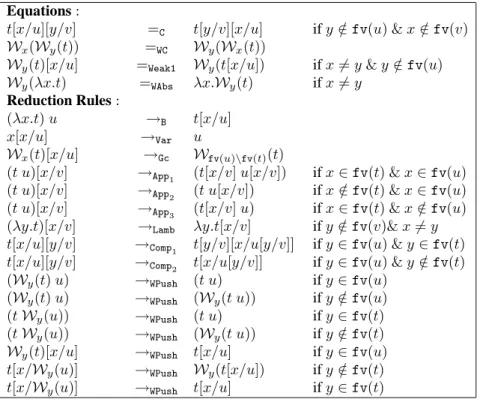
Besidesα-conversion we consider the equations and reduction rulesin Figure 3.

Equations:

t[x/u][y/v] =C t[y/v][x/u] ify /∈ fv(u) & x /∈ fv(v)

Reduction Rules:

(λx.t) u →B t[x/u]

x[x/u] →Var u

t[x/u] →Gc t ifx /∈ fv(t)

(t u)[x/v] →App1 (t[x/v] u[x/v]) ifx ∈ fv(t) & x ∈ fv(u)

(t u)[x/v] →App2 (t u[x/v]) ifx /∈ fv(t) & x ∈ fv(u)

(t u)[x/v] →App3 (t[x/v] u) ifx ∈ fv(t) & x /∈ fv(u)

(λy.t)[x/v] →Lamb λy.t[x/v] ify /∈ fv(v)

t[x/u][y/v] →Comp1 t[y/v][x/u[y/v]] ify ∈ fv(u) & y ∈ fv(t)

t[x/u][y/v] →Comp2 t[x/u[y/v]] ify ∈ fv(u) & y /∈ fv(t)

Figure 3: Equations and reduction rules forλes

The rewriting system containing all the previous rewriting rules except B is denoted by s. We write Bs for B∪ s. The equivalence relation generated by the conversions α and C is denoted by Es. The reduction relation generated by the reduction rules s (resp. Bs) modulo the equivalence relation Es is denoted by→s/Es or→es (resp.

→Bs/Esor→λes(for equational s substitution), theeis for for equational and thes for substitution. More precisely

t →est′ iff there ares, s′s.t. t =Es s →ss

′ ₌

Est ′

t →λest′ iff there ares, s′s.t. t =Es s →Bss

′₌

Es t ′

The equivalence relation preserves free variables and the reduction relation does not increase them. Indeed, one can easily show by induction on terms the following property.

Lemma 2.1 (Free variables do not increase) Ift →λest′, then fv(t′) ⊆ fv(t). More

precisely,

• If t =Est

′_{, then fv(t) = fv(t}′_).

• If t →Bst′, then fv(t′) ⊆ fv(t).

The (sub)calculus of substitutions es, which is intended to implement (meta-level) substitution can be shown to be terminating.

Lemma 2.2 (Termination of es) The reduction relation es (and thus also s) is

termi-nating.

Proof. For each terms we define a size and a multiplicity by structural induction.

S(x) := 1 Mx(z) := 1

S(λx.t) := S(t) Mx(λy.t) := Mx(t) + 1

S(t u) := S(t) + S(u) Mx(t u) := Mx(t) + Mx(u) + 1

S(t[x/u]) := S(t) + Mx(t) · S(u) Mx(t[y/u]) := Mx(t) Ifx /∈ fv(u)

Mx(t[y/u]) := Mx(t) + My(t) · (Mx(u) + 1) Ifx ∈ fv(u) Remark that Mx(s) ≥ 1 and S(s) ≥ 1 for every term s and every variable x.

We can now show, by induction on the definition of=Esand→s, that size is com-patible withα and C equality and each s-reduction step strictly decreases the size:

1. Ifs =Es s

′_{, then S(s) = S(s}′_). 2. Ifs →ss′, then S(s) > S(s′).

We then conclude that es-reduction is terminating on allλes-terms by application

of the abstract theorem A.1 : E is Es,R1 is the empty relation,R2 is→s, K is the relation given by the function S( ) and S is the standard well-founded order > on

natural numbers.

We now address the property of full composition. For that, we introduce the fol-lowing notion of substitution onλes-terms.

Givenλes-terms t and u, the result of substituting all the free occurrences of x in t by u is defined by induction, and modulo α-conversion, as follows:

x{x/v} := v

y{x/v} := y ifx 6= y (t u){x/v} := (t{x/v} u{x/v})

(λy.t){x/v} := λy.(t{x/v}) ifx 6= y and y 6∈ fv(v) t[y/u]{x/v} := t{x/v}[y/u{x/v}] ifx 6= y and y 6∈ fv(v)

It is easy to show by induction onλes-terms that t{x/u} = t if x /∈ fv(t).

Lemma 2.3 (Full Composition) Lett and u be λes-terms. Then t[x/u] →∗

λest{x/u}.

Proof. By induction ont.

3

Confluence on metaterms

Metaterms are terms containing metavariables which are usually used to denote incom-plete programs and/or proofs in higher-order unification [Hue76]. Each metavariable should come with a minimal amount of information in order to guarantee that some basic operations such as instantiation (replacement of metavariables by metaterms) is sound. Thus, we now consider a countable set of raw metavariablesX, Y, . . . that we

decorate them with sets of variablesΓ, ∆, . . ., thus yielding decorated metavariables

denoted byXΓ, Y∆, etc.

We now extend the primitive grammar forλes-terms to obtain the λes-metaterms: t ::= x | X∆| (t t) | λx.t | t[x/t]

From now on, we may useby to denote, indistinctly, a variable y or a metavariable Y_∆.

We add to the definition of free variables in Section 2 the case fv(X∆) = ∆. Even if this new definition is used to completely specify the free variables of a metaterm, which may sound contradictory with the concept of metaterm, it is worth noticing that the partial specification of the set of (free) variables of an incomplete proof says nothing about the structure of the incomplete proof itself as this structural information remains still unknown. The minimal information inside metavariables given by deco-ration of set of variables guarantees that different occurrences of the same metavariable inside a metaterm are never instantiated by different metaterms. Indeed, given the (raw) metatermt = λy.y X (λz.X), the instantiation of the (raw) metavariable X by a term

containing a free occurrence ofz would be unsound (see [Mu˜n97, DHK00, FdK] for

details).

We also extend the notion of substitution to metaterms as follows:

X_{∆{x/v} := X∆} ifx /∈ ∆ X_{∆{x/v} := X∆[x/v]} ifx ∈ ∆

Observe thatt{x/u} = t if x /∈ fv(u). Also, α-conversion is perfectly

well-defined on metaterms by extending the renaming of bound variables to the decoration sets. Thus for exampleλx.Yx=αλz.Yz.

Towards confluence by composition of substitutions The idea behind calculi with explicit substitutions having composition is to implement what is known inλ-calculus

as the substitution lemma: for allλ-terms t, u, v and variables x, y such that x 6= y and x /∈ fv(v) we have

t{x/u}{y/v} = t{y/v}{x/u{y/v}}

It is well-known that confluence on metaterms fails for calculi with ES without composition as for example the following critical pair inλx shows

s = t[y/v][x/u[y/v]]∗← ((λx.t) u)[y/v] →∗t[x/u][y/v] = s′

Indeed, while this diagram can be closed inλx for terms without metavariables [BR95],

there is no way to find a common reduct betweens and s′ _{whenevert is or contains} metavariables since no reduction rule is allowed inλx to mimic composition. Remark

that this is true not only for raw but also for decorated metavariables.

Let us now see how to close some of the interesting critical pairs inλes. For that,

let us consider the ones created from a mateterm((λx.t) u)[y/v].

Ify ∈ fv(t) & y ∈ fv(u), then

t[y/v][x/u[y/v]] ∗_{← ((λx.t) u)[y/v] → t[x/u][y/v]}

t[y/v][x/u[y/v]] ← t[x/u][y/v]

Ify ∈ fv(t) & y /∈ fv(u), then

t[y/v][x/u] ∗_{← ((λx.t) u)[y/v] → t[x/u][y/v]}

t[y/v][x/u] ≡ t[x/u][y/v]

Ify /∈ fv(t) & y ∈ fv(u), then

t[x/u[y/v]] ∗_{← ((λx.t) u)[y/v] → t[x/u][y/v]}

t[x/u[y/v]] ← t[x/u][y/v]

Ify /∈ fv(t) & y /∈ fv(u), then remark that ((λx.t) u)[y/v] cannot be reduced

further by an→Appirule so that the only possible case is

((λx.t) u) Gc← ((λx.t) u)[y/v] → t[x/u][y/v]

((λx.t) u) → t[x/u] Gc← t[x/u][y/v]

Proof techniques to show confluence While most of the calculi with explicit sub-stitutions in the literature are only specified by rewriting rules,λes-reduction is

de-fined by a notion of reduction modulo an equivalence relation. We then need to prove confluence of a non-terminating reduction relation modulo, for which the published techniques [Hue80, Ter03, Ohl98, JK86] known by the author fail. More precisely, the

untypedλes-calculus is trivially non-terminating (as it is able to simulate β-reduction),

so these techniques cannot be applied to our case since they require the reduction rela-tion to be terminating.

We now present two different proofs of confluence for metaterms. The first of them (Section 3.1) uses the technique due to Tait and Martin-L¨of [Bar84] which can be

summarised in four steps: define a simultaneous reduction relation denoted ⇛es; prove that ⇛∗_esand→∗

esare the same relation; show that ⇛∗eshas the diamond property; and use this to conclude.

The second solution (Section 3.2) consists in using a powerful version of the

in-terpretation technique [Har87]. Thus, we infer confluence ofλes from confluence of

λnss, a calculus with flattened or simultaneous substitutions whose reduction process

does not make use of any equivalence relation.

3.1

Confluence by simultaneous reduction

We first remark that the system es can be used as a function on Es-equivalence classes thanks to the following property:

Lemma 3.1 The es-normal forms of metaterms are unique modulo Es-equivalence.

Proof. We apply the proof technique in [JK86]. For that, termination of es can be shown for metaterms by extending the definitions of S and M in the proof of Lemma 2.2 as follows: S(X∆) := 1 and Mx(z) := 1. Also, es can be checked to be locally confluent and locally coherent.

A direct consequence of this lemma is thatt =Est

′_{implies es(t) =} Es es(t

′_).

Lemma 3.2 A metaterm t in es-normal form has necessarily one of the following

forms:

• t = x, or

• t = t1t2, wheret1andt2are in es-normal form.

• t = λy.t1, wheret1is in es-normal form.

• t = X∆[x1/u1] . . . [xn/un], where n ≥ 0 and every uiis in es-normal form and

xi ∈ ∆ and xi∈ fv(u/ j) for all i, j ∈ [1, n].

Lemma 3.3 Lett and u be es-normal forms. Then t{x/u} is an es-normal form.

Proof. The proof is by induction ont using Lemma 3.2.

Let consider t = X∆[x1/u1] . . . [xn/un]. By the i.h. every ui{x/u} is an es-normal form and byα-conversion we can suppose that xi ∈ fv(u). Thus, Lemma 3.2/ allows to concludet{x/u} = X∆{x/u}[x1/u1{x/u}] . . . [xn/un{x/u}] is in es-normal form.

All the other ones are straightforward.

Lemma 3.4 Lett, u, v be es-normal forms and suppose x /∈ fv(v). Then t{x/u}{y/v} =Es

t{y/v}{x/u{y/v}}.

Lemma 3.5 Lett, u, v be λes-terms. Then es((t u)[x/v]) = es(t[x/v]) es(u[x/v]).

Proof. By cases.

Ifx ∈ fv(t) & x ∈ fv(u), then (t u)[x/v] →App1 t[x/v] u[x/v].

Ifx /∈ fv(t) & x ∈ fv(u), then (t u)[x/v] →App2 t u[x/v]Gc← t[x/v] u[x/v]. Ifx ∈ fv(t) & x /∈ fv(u), then (t u)[x/v] →App3 t[x/v] uGc← t[x/v] u[x/v]. Ifx /∈ fv(t) & x /∈ fv(u), then (t u)[x/v] →Gct u∗Gc← t[x/v] u[x/v]. Thus, in all cases the property holds.

Lemma 3.6 Lett, u, v be λes-terms. Then es(t[x/u][y/v]) =Es es(t[y/v][x/u[y/v]]). Proof. By cases.

Ify ∈ fv(t) & y ∈ fv(u), then t[x/u][y/v] →Comp1t[y/v][x/u[y/v]].

Ify /∈ fv(t) & y ∈ fv(u), then t[x/u][y/v] →Comp2 t[x/u[y/v]]Gc← t[y/v][x/u[y/v]]. Ify ∈ fv(t) & y /∈ fv(u), then t[x/u][y/v] =Es t[y/v][x/u]Gc← t[y/v][x/u[y/v]]. Ify /∈ fv(t) & y /∈ fv(u), then t[x/u][y/v] →Gct[x/u]∗Gc← t[y/v][x/u[y/v]].

Lemma 3.7 Lett and u be meta λes-terms. Then es(t[x/u]) = es(t){x/es(u)}.

Proof. The proof is by induction ont using Lemmas 3.5, 3.6 and 3.3.

Lemma 3.8 Let t, t′_{, u, u}′ _{be es-normal forms. If t =} Es t ′ _{and u =} Es u ′_{, then} t{x/u} =Est ′_{x/u′_}. Proof. By induction ont.

The simultaneous reduction

We now introduce the simultaneous reduction relation ⇛eson es-normal forms which is given by a simpler relation ⇛ modulo Es-equivalence.

Definition 3.1 (The relations ⇛ and ⇛es) The relation ⇛ is defined on metaterms

in es-normal forms:

• x ⇛ x

• If t ⇛ t′_{, thenλx.t ⇛ λx.t}′

• If t ⇛ t′_{andu ⇛ u}′_{, thent u ⇛ t}′_u′

• If t ⇛ t′_{andu ⇛ u}′_{, then(λx.t) u ⇛ es(t}′_[x/u′_])

• If ui⇛u′iandxi∈ fv(u/ j) for all i, j ∈ [1, n], then X∆[x1/u1] . . . [xn/un] ⇛

X_∆[x1/u′_{1] . . . [xn/u}′_n]

Now we define the following reduction relation

t ⇛est′iff there ares, s′s.t. t =Es s ⇛ s

′₌

Est ′

The following properties are straightforward.

Remark 3.9

• t ⇛ t for every es-normal form t.

• ⇛esis closed by contexts: ifti⇛est′ifori ∈ [1, n], then u = C[t1, . . . , tn] ⇛es

C[t′

1, . . . , t′n] = u′wheneveru and u′are es-normal forms.

• If t ⇛ t′_{, then then es(t) ⇛ es(t}′_).

Lemma 3.10 ⇛∗_es⊆→∗ λes.

Proof. It is sufficient to show ⇛∗⊆→∗_{. This can be done on induction on the}

number of steps in ⇛∗, then by induction on the definition of ⇛. A consequence of this lemma is thatt ⇛est′implies fv(t′) ⊆ fv(t).

Lemma 3.11 Ift1⇛est′1andt2⇛est2′, then(λx.t1) t2⇛eses(t′1[x/t′2]).

Proof. Let consider t1 =Es u1 ⇛ u

′ 1 = Est′1 and t2 =Es u2 ⇛es u ′ 2 =Es t′2. We haveu′1[x/u′2] =Es t ′

1[x/t′2] so that es(u′1[x/u′2]) =Es es(t ′ 1[x/t′2]). Then (λx.t1) t2=Es(λx.u1) u2⇛es(u ′ 1[x/u′2]) =Es es(t ′ 1[x/t′2]).

Lemma 3.12 Ift ⇛ t′_{andu ⇛ u}′_{, then es(t[x/u]) ⇛}

eses(t′[x/u′]).

Proof. By induction ont ⇛ t′_.

• If x ⇛ x, then es(x[x/u]) = es(u) ⇛ es(u′_{) = es(x[x/u}′_{]) holds by} Re-mark 3.9.

• If y ⇛ y, then es(y[x/u]) = y ⇛ y = es(y[x/u′_{]) holds by definition.}

• If t1t2⇛t′1t′2, wheret1⇛t′1andt2⇛t′2, then

es((t1t2)[x/u]) = (L. 3.5)

es(t1[x/u]) es(t2[x/u]) ⇛es(i.h.)

es(t′1[x/u′]) es(t′2[x/u′]) = (L. 3.5)

es((t′

1t′2)[x/u′])

• If λy.v ⇛ λy.v′_{, wherev ⇛ v}′_{, then}

es((λy.v)[x/u]) =

λy.es(v[x/u]) ⇛_es(i.h.) λy.es(v′_[x/u′_{]) =}

• If (λy.t1) v ⇛ es(t′1[y/v′]), where t1⇛t′1andv ⇛ v′, then

es(((λy.t1) v)[x/u]) = (L. 3.5)

es((λy.t1)[x/u]) es(v[x/u]) =

(λy.es(t1[x/u])) es(v[x/u]) ⇛es(i.h. and L. 3.11)

es(es(t′

1[x/u′])[y/es(v′[x/u′])]) =

es(t′

1[x/u′][y/v′[x/u′]]) =Es(L. 3.6)

es(t′

1[y/v′][x/u′]) =

es(es(t′

1[y/v′])[x/u′])

• If X∆[x1/u1] . . . [xn/un] ⇛ X∆[x1/u1′] . . . [xn/u′n], where ui ⇛u′iandxi ∈/

fv(uj) for all i, j ∈ [1, n], then we reason by induction on n.

– Forn = 0 we have two cases.

Ifx /∈ ∆, then es(X∆[x/u]) = X∆⇛ X∆= es(X∆[x/u′]).

Ifx ∈ ∆, then es(X∆[x/u]) = X∆[x/es(u)] ⇛ X∆[x/es(u′)] = es(X∆[x/u′]).

– Forn > 0 we consider the following cases.

Ifx /∈ fv(X∆[x1/u1] . . . [xn/un]), then also x /∈ fv(X∆[x1/u′1] . . . [xn/u′n]) and thus es(X∆[x1/u1] . . . [xn/un][x/u]) = X_{∆[x1/u1] . . . [xn/un]} ⇛ X_∆[x1/u′_{1] . . . [xn/u}′_n] = es(X∆[x1/u′1] . . . [xn/u′n][x/u]) Ifx ∈ fv(X∆[x1/u1] . . . [xn/un]), then let i be the greatest number such that x ∈ fv(ui) so that x /∈ fv(ui+1) . . . fv(un) and thus also x /∈

fv(u′i+1) . . . fv(u′n). Two cases are possible.

Ifx /∈ fv(X∆[x1/u1] . . . [xi−1/ui−1]), then also x /∈ fv(X∆[x1/u′1] . . . [xi−1/u′i−1])

es(X∆[x1/u1] . . . [xn/un][x/u]) =Es

es(X∆[x1/u1] . . . [xi/ui][x/u][xi+1/ui+1] . . . [xn/un]) =

es(X∆[x1/u1] . . . [xi/ui[x/u]][xi+1/ui+1] . . . [xn/un]) =

X_{∆[x1/u1] . . . [xi/es(ui[x/u])][xi+1/ui+1] . . . [xn/un]} ⇛_es(first i.h.) X_{∆[x1/u1] . . . [xi/es(u}′_i[x/u′_])][xi+1/u′_{i+1] . . . [xn/u}′_{n]) =E}

s

es(X∆[x1/u′1] . . . [xn/u′n][x/u′])

Ifx ∈ fv(X∆[x1/u1] . . . [xi−1/ui−1]), then

es(X∆[x1/u1] . . . [xn/un][x/u]) =Es

es(X∆[x1/u1] . . . [xi/ui][x/u][xi+1/ui+1] . . . [xn/un]) =

es(X∆[x1/u1] . . . [xi−1/ui−1][x/u][xi/ui[x/u]][xi+1/ui+1] . . . [xn/un]) =

By the first i.h. we have es(ui[x/u]) ⇛eses(u′i[x/u′]) and by the second

i.h. we have es(X∆[x1/u1] . . . [xi−1/ui−1][x/u]) ⇛eses(X∆[x1/u′1] . . . [xi−1/u′i−1][x/u′]). Thus,

es(X∆[x1/u1] . . . [xi−1/ui−1][x/u])[xi/es(ui[x/u])][xi+1/ui+1] . . . [xn/un] ⇛es

es(X∆[x1/u′1] . . . [xi−1/u′i−1][x/u′])[xi/es(u′i[x/u′])][xi+1/u′i+1] . . . [xn/u′n] =

es(X∆[x1/u′1] . . . [xi−1/u′i−1][x/u′][xi/ui′[x/u′]])[xi+1/u′i+1] . . . [xn/u′n] =Es (L. 3.6)

es(X∆[x1/u′1] . . . [xi−1/u′i−1][xi/ui′][x/u′])[xi+1/u′i+1] . . . [xn/u′n] =Es

es(X∆[x1/u′1] . . . [xi−1/u′i−1][xi/u′i][xi+1/u′i+1] . . . [xn/u′n][x/u′])

Corollary 3.13 Ift ⇛est′andu ⇛es u′, then es(t[x/u]) ⇛eses(t′[x/u′]).

Proof. Lett =Es t1 ⇛ t2 =Es t

′ _{andu =}

Es u1 ⇛ u2 =Es u

′_{so thatt[x/u] =} Es

t1[x/u1] and t2[x/u2] =Es t

′_[x/u′_{]. By Lemma 3.12 we have}

es(t[x/u]) =Es es(t1[x/u1]) ⇛eses(t2[x/u2]) =Es es(t ′_[x/u′_]) Thus we conclude es(t[x/u]) ⇛eses(t′[x/u′]).

Lemma 3.14 →λes⊆⇛es Proof. Ifs →es s′, then s =Es t →es t ′ ₌ Es s ′ _{so that es(s) =} Es es(t) =Es es(t′_{) =} Es es(s

′_{) holds by Lemma 3.1. By definition es(s) =}

Es es(t) ⇛ es(t) =Es

es(t′_{) =} Es es(s

′_{). Thus, es(s) ⇛}

eses(s′) by definition.

Now one shows that s →B s′ implies es(s) ⇛es es(s′) by induction on s and using Remark 3.9 and Corollary 3.13. We then have thats =Es s1 →B s2 =Es s

′ implies es(s) =Es es(s1) ⇛eses(s2) =Es es(s

′_).

Finally, one concludes thats →λess′implies es(s) ⇛eses(s′).

Lemma 3.15 The relation ⇛eshas the diamond property, that is, ift1 es⇚t ⇛est2,

then there ist3such thatt1⇛est3 es⇚t2. 1. We first provet ⇚ u =Es u ′_{impliest =} Es t ′ _⇚u′_. Proof. By induction ont ⇚ u. • x ⇚ x =Es x • λx.t ⇚ λx.u =Esλx.u ′_{, wheret ⇚ u =} Es u ′_. • t1t2 ⇚u1u2=Es u ′ 1u′2, wheret1 ⇚u1=Es u ′ 1andt2 ⇚u2=Es u ′ 2 • X∆[x1/t1] . . . [xn/tn] ⇚ X∆[x1/u1] . . . [xn/un] =Es X∆[xπ(1)/u ′ π(1)] . . . [xπ(n)/u′π(n)], whereti ⇚ui=Esu ′

i. By the i.h. we haveti=Es t ′ i ⇚u′iso that we close the diagram by X_{∆[x1/t1] . . . [xn/tn] =E} s X_∆[x1/t′ 1] . . . [xn/t′n] =Es X_∆[xπ(1)/t′ π(1)] . . . [xπ(n)/t′π(n)] ⇚ X_∆[xπ(1)/u′ π(1)] . . . [xπ(n)/u′π(n)]

• es(t1[x/t2]) ⇚ (λx.t1) t2=Es (λx.t ′ 1) t′2wheret1=Es t ′ 1andt2=Es t ′ 2. We havet1[x/t2] =Es t ′

1[x/t′2] so that we close the diagram by

es(t1[x/t2]) =Es es(t ′ 1[x/t′2]) ⇚ (λx.t′1) t′2 2. We proveves⇚v′=Es u ′_{impliesv =} Es t ′ _⇚u′_. Proof. Ifv es⇚v′ =Es u ′_{, thenv =} Es t ⇚ u =Es v ′ ₌ Es u ′ _{so thatv =} Es t ⇚ u =Es u

′_{. By the previous pont there ist}′ _{such thatt =} Es t

′ _⇚u′_{. Then}

v =Es t ′ _⇚u′_.

3. We provet1 ⇚t ⇛ t2impliest1⇛est3 es⇚t2.

Proof. The proof is by induction on the definition of ⇛.

• Let us consider

(λx.t1) u1 ⇚(λx.t) u ⇛ es(t2[x/u2])

wheret ⇛ t1andt ⇛ t2andu ⇛ u1andu ⇛ u2. By the i.h. we know there aret3andu3such thatt1⇛est3andt2 ⇛es t3andu1⇛esu3and

u2⇛esu3so that in particulart1=Esw1⇛w3=Es t3andu1=Es w ′ 1⇛ w′ 3=Esu3. We have (λx.t1) u1=Es(λx.w1) w ′

1⇛es(w3[x/w3′]) =Eses(t3[x/u3]) and Corollary 3.13 gives

es(t2[x/u2]) ⇛eses(t3[x/u3])

• Let us consider

es(t1[x/u1]) ⇚ (λx.t) u ⇛ es(t2[x/u2])

wheret ⇛ t1andt ⇛ t2andu ⇛ u1andu ⇛ u2. By the i.h. we know there aret3andu3such thatt1⇛est3andt2 ⇛es t3andu1⇛esu3and

u2⇛esu3. Then, Corollary 3.13 gives

es(t1[x/u1]) ⇛eses(t3[x/u3])es⇚es(t2[x/u2])

4. We provet1 es⇚t ⇛est2impliest1⇛est3 es⇚t2.

Proof. Lett1 es⇚t =Es u ⇛ u

′ ₌

Es t2. By the second point there isu1such thatt1=Es u1 ⇚u and by the third point there is t3such thatu1⇛est3 es⇚u

′_. We concludet1⇛est3 es⇚t2.

Corollary 3.16 The reduction relation→∗

esis confluent.

Proof. Any relation enjoying the diamond property can be shown to be conflu-ent [] so that the reduction relation ⇛∗_es does. We also remark that ⇛∗_es and→∗

λes are the same relation so that→∗

λesturns to be also confluent. Indeed, ⇛∗es⊆→∗λesby Lemma 3.10 and→∗

λes⊆⇛∗esby several applications of Lemma 3.14.

3.2

Confluence by interpretation

We present a second proof of confluence for metaterms. For that, we first define a calculus with simultaneous substitution whose reduction process does not make use of any equivalence relation.

3.2.1 A calculus with simultaneous substitution

We consider here a dense order on the set of variablesX . Renaming is assumed to be

order preserving.

We then define ss-metaterms as metaterms withn-ary substitutions used to denote

simultaneous substitutions. The grammar can be given by:

t ::= x | X∆| (t t) | λx.t | t[xk1/t, . . . , xkn/t]

where substitutions [xk1/uk1. . . , xkn/ukn] are non-empty (so that n ≥ 1) and

xk1, . . . , xknare all distinct variables.

Remark that no order exist in the general syntax between the distinct variables of a simultaneous substitution.

We use lettersI, J, K to denote non-empty lists of indexes for variables and I@J

to denote concatenation of the listsI and J. If I is the list k1. . . kn, then we write

[xi/ui]I for the list[xk1/uk1, . . . , xkn/ukn]. We might also use the notation [lst] for any of such (non-empty) lists and[cs[[x/t]]i]I for a simultaneous substitution of

I elements containing x/t at position i ∈ I. Given [xi/ui]I, we use the notation

[xi/ui]I+to denote the substitution where an element has been added at the end of the listxk1/u1, . . . , xkn/unand[xi/ui]+I to denote the substitution where an element has been added at the beginning of the list.

Ifj ∈ I and |I| ≥ 2, we write [xi/ui]I\jfor the list[xk1/uk1, . . . , xkn/ukn] whose elementxj/uj has been erased. Thus for examplex[x2/z, x3/w] can be written as

x[xi/ui][2,3]withk1= 2, k2= 3, u2= z and u3= w and x[xi/ui][2,1]\2denotes the termx[x3/w].

For any permutationπ(I), the notation [xi/ui]π(I) denotes the (permutated) list

[xπ(k1)/uπ(k1), . . . , xπ(kn)/uπ(kn)]. Thus for example, if I = k1. . . knand sort(I) =

Definition 3.2 (Free and bound variables) Free and bound variables of ss-metaterms

are defined by induction as follows:

fv(x) := {x} fv(X∆) := ∆ fv(t u) := fv(u) ∪ fv(u) fv(λx.t) := fv(t) \ {x} fv(t[xk1/uk1, . . . , xkn/ukn]) := fv(t) \ {xk1, . . . , xkn} ∪ fv(uk1) . . . ∪ fv(ukn) bv(x) := ∅ bv(X∆) := ∅ bv(t u) := bv(u) ∪ bv(u) bv(λx.t) := bv(t) ∪ {x} bv(t[xk1/uk1, . . . , xkn/ukn]) := bv(t) ∪ {xk1, . . . , xkn} ∪ bv(uk1) . . . ∪ bv(ukn) As before, we work modulo alpha conversion so we assume all bound variables are distinct and no variable is bound and free at the same time. As a consequence, for any term of the formt[xk1/uk1, . . . , xkn/ukn] we have xki ∈ fv(u/ kj) for all 1 ≤ i, j ≤ n. The following reduction systemF is used to transform successive depending unary

substitutions into one single (flattened) simultaneous substitution.

(t u)[lst] →fl1 t[lst] u[lst]

(λx.t)[lst] →fl2 λx.t[lst]

t[xi/ui]I[yj/vj]J →fl3 t[xi/ui[yj/vj]J, yj/vj]I@J

t[xi/ui]I →fl4 t[xi/ui]sort(I) ifI is not sorted

Figure 4: Reduction rules forF

Note that byα-conversion there is no capture of variable in the rules fl2and fl4. As an example we have

(x[x4/x3, x2/z] y)[x3/w] →fl1

(x[x4/x3, x2/z][x3/w] y[x3/w]) →fl3

(x[x4/x3[x3/w], x2/z[x3/w], x3/w] y[x3/w]) →fl4

(x[x2/z[x3/w], x3/w, x4/x3[x3/w]] y[x3/w])

The systemF can be considered as a functional specification thanks to the

follow-ing property.

Lemma 3.17 The systemF is confluent and terminating on ss-metaterms.

Proof. Confluence can be shown using the development closed confluence tech-nique in [Ter03]. Termination can be shown using for example a semantic (for the sorting) Lexicographic Path Ordering [Ter03].

From now on, we denote byF(t) the F-normal form of t.

Observe thatt →Ft′implies fv(t) = fv(t′) so that fv(F(t)) = fv(t).

The following property will be useful in the rest of this section, it can be shown by induction on ss-metaterms.

Lemma 3.18 (F-normal forms) The set nf(F) of ss-metaterms that are in F-normal

form can be characterised by the following inductive definition.

• If ui∈ nf(F) for all i ∈ I and by is a variable or a metavariable and I is sorted,

theny[xb i/ui]I ∈ nf(F).

• If u ∈ nf(F), then λx.u ∈ nf(F) • If u, v ∈ nf(F), then (u v) ∈ nf(F)

3.2.2 A calculus with normal simultaneous substitutions

Theλnss-metaterms are defined as the subset of the ss-metaterms that are in F-normal

form. Thecalculus is defined by the following set of reduction rules on

λnss-metaterms.

(λx.t) u →n1 F(t[x/u])

xj[xi/ui]I →n2 uj j ∈ I

t[xi/ui]I →n3 t[xi/ui]I\j j ∈ I & xj∈ fv(t)/

t[x/u] →n4 t x /∈ fv(t)

Figure 5: Reduction rules for theλnss-calculus

Note that the n4 is a particular case of n3, but we have to specify it separately because we choose to avoid the use of empty substitutions.

Theλnss-reduction relation is defined by induction as follows. • If t →n1,n2,n3,n4t′, thent →λnsst′.

• If t →λnsst′, thenλx.t →λnssλx.t′.

• If t →λnsst′, then(t u) →λnss(t′u) and (u t) →λnss(u t′).

• If u →λnssu′andj ∈ I, then y[cs[[x/u]]j]I →λnssy[cs[[x/u′]]j]Iand Y∆[cs[[x/u]]j]I →λnss

Y_∆[cs[[x/u′_]]j]I.

As expected, the reduction system is well-defined in the sense thatt ∈ nf(F) and t →λnsst′impliest′ ∈ nf(F).

Here is an example ofλnss-reduction, where we assume y < x. (λx.x ((λy.y) w)) z →n1 x[x/z] ((λy.y[x/z]) w[x/z]) →n1 x[x/z] y[y/w[x/z], x/z[y/w[x/z]]] →n2 x y[y/w[x/z], x/z[y/w[x/z]]] →n4 x y[y/w[x/z], x/z] →n3 x y[y/w[x/z]] →n2 x w[x/z] →n4 x w

As expected, theλnss-calculus enjoys confluence

Theorem 3.20 (λnss is confluent) The relation λnss is confluent on metaterms.

Proof. Confluence can be shown using the development closed confluence theorem in [Ter03].

3.2.3 Relatingλes and λnss

We now establish a correspondence betweenλes and λnss-reduction which will be

used in the interpretation proof of confluence forλes.

We first need the following lemma.

Lemma 3.21 Letv and ui(i ∈ I) be ss-terms.

1. Ifj ∈ I, where |I| ≥ 2 and xj∈ fv(v), then F(v[x/ i/ui]I) →+λnssF(v[xi/ui]I\j).

2. Ifx /∈ fv(v), then F(v[x/u]) →+

λnssF(v).

Proof. We can reason by induction onv.

Theλnss-reduction relation is stable by closure followed by flattening, that is,

Lemma 3.22 Letv be a ss-terms and t1, t2beF-normal forms. If t1→λnsst2, then

1. F(t1) →+λnssF(t2)

2. F(t1[x/v]) →+_λnssF(t2[x/v])

3. F(v[cs[[x/t1]]i]I) →+_λnssF(v[cs[[x/t2]]i]I).

Proof. We can show the first and second properties by induction onλnss and the

third one by induction onv.

We are now ready to simulateλes-reduction into the system λnss via the flattening

Theorem 3.23 Ift →λest′, thenF(t) →∗_λnssF(t′) .

Proof. We proceed by induction. If the reduction is internal, andt is an application

or an abstraction, then the proof is straightforward. Ift = t1[x/v] is a closure and

t′ _{= t}

2[x/v], then F(t1) →∗λnss F(t2) by i.h. and F(t) = F(F(t1)[x/v]) →∗λnss

F(F(t2)[x/v]) holds by Lemma 3.22:2. If t = v[x/t1] is a closure and t′ = v[x/t2], thenF(t1) →∗λnss F(t2) by i.h. and F(t) = F(v[x/F(t1)]) →∗λnss F(v[x/F(t2)]) holds by Lemma 3.22:3. If the reduction is external we have to inspect all the possible cases.

We can then conclude

Corollary 3.24 Ift →∗λes t′, thenF(t) →∗λnssF(t′).

3.2.4 Relatingλnss and λes

We have projectedλes-reductions steps into λnss-reduction steps but we also need

to prove that the projection in the other way around is possible too. This will be the second important ingredient of the interpretation proof of confluence that we present at the end of this section.

In order to translateλnss into λes we define the following sequentialisation

func-tion.

seq(x) := x

seq(t u) := seq(t) seq(u) seq(λx.t) := λx.seq(t)

seq(t[xi/ui]I) := seq(t) if everyxi∈ fv(seq(t))/

seq(t[xi/ui]I) := seq(t)[xi/seq(ui)]K

whereK is the biggest non empty sublist of I such that for all k ∈ K the variable xkis free in seq(t).

We remark that fv(seq(t)) ⊆ fv(t).

As expected, the system seq can be used to projectF-reduction (Theorem 3.25)

andλnss-reduction (Theorem 3.26) into λes-reduction.

Theorem 3.25 Ifs and s′_{are ss-terms such thats →}

F s′, then seq(s) →∗λesseq(s′).

Proof. By induction on the reductionF. If the reduction is internal the property is

straightforward. Otherwise we have to inspect all the possible cases.

Theorem 3.26 Ifs →λnsss′, then seq(s) →∗λesseq(s′)

Proof. By induction on →λnss. The cases where the reduction is internal are

straightforward so we have to inspect the cases of external reductions.

F (t) = F (t′₎ seq(t2) * * * * * seq(F (t2)) t3 t=Est ′ t2 F (t1) * * * t1 F (t2) * * * seq(t1) seq(F (t1)) * * seq(t3) *

Figure 6: Confluence proof forλes on metaterms

Corollary 3.27 The systemλes is confluent on metaterms.

Proof. Let t ≡ t′_{, t →}∗

λes t1 and t′ →∗λes t2. By Theorem 3.23 we have

F(t) = F(t′_{) and F (t) →}∗

λnss F(t1) and F (t′) →∗λnss F(t2). Theorem 3.20 gives confluence ofλnss on F -normal forms so that there is an F -normal form t3 such that F(t1) →∗λnss t3 andF(t2) →∗λnss t3. Now, t1 →∗_F F(t1) and t2 →∗_F

F(t2) imply seq(t1) →∗λes seq(F (t1)) and seq(t2) →∗λes seq(F (t2)) by Theo-rem 3.25. But seq(t1) = Gc(t1) and seq(t2) = Gc(t2) so that t1 →∗λes seq(t1) and

t2→∗λesseq(t2). Theorem 3.26 allows us to conclude seq(F (t1)) →∗λesseq(t3) and

seq(F (t2)) →∗_λesseq(t3) which closes the diagram.

4

Preservation of β-strong normalisation

Preservation ofβ-strong normalisation (PSN) in calculi with explicit substitutions

re-ceived a lot of attention (see for example [ACCL91, BBLRD96, BR95, KR95]), start-ing from an unexpected result given by Melli`es [Mel95] who has shown that there are

β-strongly normalisable terms in λ-calculus that are not strongly normalisable when

evaluated by the reduction rules of an explicit version of theλ-calculus. This is for

example the case ofλσ [ACCL91] or λσ⇑[HL89].

This phenomenon shows a flaw in the design of these calculi with explicit substi-tutions in that they are supposed to implement their underlying calculus without losing its good properties. However, there are many ways to avoid Melli`es’ counter-example in order to recover the PSN property. One of them is to simply forbid the substitu-tion operators to cross lambda-abstracsubstitu-tions [LM99, For02]; another consists of

avoid-ing composition of substitutions [BBLRD96]; another one imposes a simple strategy on the calculus with explicit substitutions to mimic exactly the calculus without ex-plicit substitutions [GL99]. The first solution leads to weak lambda calculi, not able to express strong beta-equality, which is used for example in implementations of proof-assistants [Coq, HOL]. The second solution is drastic as composition of substitutions is needed in implementations of HO unification [DHK95] or functional abstract ma-chines [HMP96]. The last one exploits very little of the notion of explicit substitutions because they can be neither composed nor even delayed.

In order to cope with this problem David and Guillaume [DG01] defined a calculus with labels, calledλws, which allows controlled composition of explicit substitutions without losing PSN. These labels can be also seen as special annotations induced by a logical weakening rule. Another solution, calledλlxr, has been introduced latter

by Kesner and Lengrand [KL05], the idea is the complete control of resources, so that not only for weakening, but also for contraction. Anyway, both calculi can be translated to Linear Logic’s proof-nets [DCKP03, KL05], underlying in this way the key points where composition of substitutions must be controlled. The calculusλws as well asλlxr introduces new syntax to handle composition. The claim of this

pa-per is that explicit resources as weakening and contraction are not necessary to define composition correctly. Indeed, whileλlxr-reduction is defined via 6 equations and 19 rewriting rules, λes only uses an equation for commutativity of substitutions and 9

natural rewriting rules.

Preservation ofβ-strong normalisation is quite difficult to prove in calculi with

composition (see for example [Blo97, DG01, ABR00, KL05, KOvO01]). This is mainly because the so-called decent terms are not stable by reduction : a termt is

said to be decent in the calculusZ if every subterm v appearing as body of some

sub-stitution (i.e. appearing in some subtermu[x/v] of t) is Z-strongly normalising. As an

example, the termx[x/(y y)][y/λw.(w w)] is decent in λes since (y y) and λw.(w w)

areλes-strongly normalising, but its Comp₂-reductx[x/(y y)[y/λw.(w w)] is not since (y y)[y/λw.(w w)] is not λes-strongly normalising.

In this paper we prove thatλes preserves β-strong normalisation by using a proof

technique based on simulation. The following steps will be developed 1. We define a new calculusλesw (section 4.1).

2. We define a translation K fromλes-terms (and thus also from λ-terms) to λesw

such that

(a) t ∈ SNβimplies K(t) ∈ SNλesw(Corollary 4.15). (b) K(t) ∈ SNλeswimpliest ∈ SNλes(Corollary 4.6).

4.1

The λesw-calculus

We introduce here theλesw-calculus, an intermediate language between λes and λlxr [KL05],

which will be used as technical tool to prove PSN. The grammar ofλesw-terms is given as follows:

We will only consider here strict terms: every subtermλx.t and t[x/u] is such that x ∈ fv(t) and every subterm Wx(t) is such that x /∈ fv(t). We use the abbreviation

WΓ(t) for Wx1(. . . Wxn(t)) whenever Γ = {x1, . . . , xn}. In the particular case Γ is the empty set the notationW_∅(t) = t.

Besides α-conversion we consider the equations and and reduction rules in

Fig-ure 7.

Equations:

t[x/u][y/v] =C t[y/v][x/u] ify /∈ fv(u) & x /∈ fv(v)

Wx(Wy(t)) =WC Wy(Wx(t))

Wy(t)[x/u] =Weak1 Wy(t[x/u]) ifx 6= y & y /∈ fv(u)

Wy(λx.t) =WAbs λx.Wy(t) ifx 6= y

Reduction Rules:

(λx.t) u →B t[x/u]

x[x/u] →Var u

Wx(t)[x/u] →Gc Wfv(u)\fv(t)(t)

(t u)[x/v] →App1 (t[x/v] u[x/v]) ifx ∈ fv(t) & x ∈ fv(u)

(t u)[x/v] →App2 (t u[x/v]) ifx /∈ fv(t) & x ∈ fv(u)

(t u)[x/v] →App3 (t[x/v] u) ifx ∈ fv(t) & x /∈ fv(u)

(λy.t)[x/v] →Lamb λy.t[x/v] ify /∈ fv(v)& x 6= y

t[x/u][y/v] →Comp1 t[y/v][x/u[y/v]] ify ∈ fv(u) & y ∈ fv(t)

t[x/u][y/v] →Comp2 t[x/u[y/v]] ify ∈ fv(u) & y /∈ fv(t)

(Wy(t) u) →WPush (t u) ify ∈ fv(u)

(Wy(t) u) →WPush (Wy(t u)) ify /∈ fv(u)

(t Wy(u)) →WPush (t u) ify ∈ fv(t)

(t Wy(u)) →WPush (Wy(t u)) ify /∈ fv(t)

Wy(t)[x/u] →WPush t[x/u] ify ∈ fv(u)

t[x/Wy(u)] →WPush Wy(t[x/u]) ify /∈ fv(t)

t[x/Wy(u)] →WPush t[x/u] ify ∈ fv(t)

Figure 7: Equations and Reduction rules forλesw

The rewriting system containing all the previous rewriting rules except B is denoted by sw. We write Bsw for B∪sw. The equivalence relation generated by all the equations

is denoted by Esw. The relation generated by the reduction rules sw (resp. Bsw) modulo the equivalence relation Esw is denoted by→sw /Esw or →esw (resp. →Bsw /Esw or

→λesw). More precisely

t →eswt′ iff there ares, s′s.t. t =Esw s →sws

′₌

Esw t ′

t →λeswt′ iff there ares, s′s.t. t =Esw s →Bsws

′ ₌

Eswt ′ The following lemma can be proved by induction on terms.

The following property can be shown by induction on terms.

From now on, we only work with strict terms.

We proceed now to show that esw is a terminating system. We will do this in two steps: first we show that→esw minus→WPush is terminating (Lemma 4.2), then we show that→WPush / =Esw is terminating (Lemma 4.3). All this allows us to conclude (Corollary 4.4) that the whole system→eswis terminating.

We will need the following measure for terms.

Definition 4.1 For eachλesw-term s we define a size and a multiplicity by structural

induction. S(x) := 1 Mx(z) := 1 S(Wx(t)) := S(t) Mx(Wy(t)) := Mx(t) Mx(Wx(t)) := 1 S(λx.t) := S(t) Mx(λy.t) := Mx(t) + 1 S(t u) := S(t) + S(u) Mx(t u) := Mx(t) + Mx(u) + 1

S(t[x/u]) := S(t) + Mx(t) · S(u) Mx(t[y/u]) := Mx(t) Ifx /∈ fv(u)

Mx(t[y/u]) := Mx(t) + My(t) · (Mx(u) + 1) Ifx ∈ fv(u) Remark that Mx(s) ≥ 1 and S(s) ≥ 1 for every term s and every variable x.

This measure enjoys the following property:

Lemma 4.2 Lets, s′_{beλrxw-terms.}

1. Ifs =Esw s

′_{, then S(s) = S(s}′_).

2. Ifs →WPushs′, then S(s) = S(s′).

3. Ifs →sw\WPushs′, then S(s) > S(s′).

Proof. The proof is by induction on→esw.

Lemma 4.3 →WPush/Eswis a terminating system.

Proof. For each terms we define a measure P(s) by induction as follows:

P(x) := 1

P(t u) := 2 · P(t) + 2 · P(u) P(λx.t) := P(t) + 1

P(Wx(t)) = P(t) + 1

P(t[x/u]) := P(t) + 2 · P(u)

Remark that P(s) ≥ 1 for every s.

Now, givens we consider hnbw(s), P(s)i, where nbw(s) is the number of

weaken-ings ins. We show that s →WPush/Esw s

′_{implieshnbw(s), P(s)i >}

lexhnbw(s′), P(s′)i. The proof proceeds by induction on→WPush/Esw.

We can then conclude that{WPush}/Esw-reduction is terminating on allλesw-terms by application of the abstract theorem A.1 : E is Esw,R1is the empty relation,R2is

→WPush, K is the relation given by the measurehnbw( ), P( )i and S is >lex which is the standard (well-founded) lexicographic order on N× N.

In order to conclude with that the whole system esw is terminating on all

λesw-terms we apply again Theorem A.1:E is Esw,R1is the relation→WPush(so that→WPush

/Eswis well-founded by Lemma 4.3), K is the relation given by the function S( ), R2is the relation→_sw\{WPush}which strictly decreases the measure S( ) by Lemma 4.2 and S is the standard well-founded order > on N.

Corollary 4.4 The reduction relation esw is terminating.

4.2

Relating λes and λesw

The aim of this section is to relateλes and λesw-reduction in order to infer

thatλesw-normalisation impliesλes-normalisation.

We start by giving a translation fromλes-terms to λesw-terms which introduces as

many weakening constructors as is necessary to build strictλesw-terms.

Definition 4.2 (Fromλes-terms to (strict λesw-terms) The translation from λes-terms

(and thus also fromλ-terms) to strict λesw-terms is defined by induction as follows:

K(x) = x K(u v) = K(u) K(v) K(λx.t) = λx.K(t) Ifx ∈ fv(t) K(λx.t) = λx.Wx(K(t)) Ifx /∈ fv(t) K(u[x/v]) = K(u)[x/K(v)] Ifx ∈ fv(t) K(u[x/v]) = Wx(K(u))[x/K(v)] Ifx /∈ fv(t) Remark that fv(K(t)) = fv(t).

The relevant point to relate nowλes and λesw-reduction consists in pulling out

weakening constructors:

Lemma 4.5 Ifs →λes s′, then K(s) →+λeswWfv(s)\fv(s′)(K(s′)).

Proof. By induction on→λes.

It is worth noticing that we really need in this proof Weak1 and WAbs as equations and not as rewriting rules.

We can then now conclude this part with the main result of this section.

Corollary 4.6 If K(t) ∈ SNλesw, thent ∈ SNλes.

4.3

The

Λ

-calculus

Definition 4.3 The setΛIof terms of theλI-calculus [Klo80] is defined by the

follow-ing grammar:

We only consider strict terms: every subtermλx.M satisfies x ∈ fv(M ).

We use[N, hM i] or [N, M1, M2, . . . , Mn] to denote the term [. . . [[N, M1], M2], . . . , Mn] assuming that this expression is equal toN when n = 0. The term M and the notation hM i inside [N, hM i] must not be confused.

As in the λ-calculus, the following property is straightforward by induction on

terms.

Lemma 4.7 (Substitutions [Klo80]) For allΛI-termsM, N, L, we have M {x/N } ∈

ΛI andM {x/N }{y/L} = M {y/L}{x/N {y/L}} provided there is no variable

cap-ture.

In what follows we consider two reduction rules onΛI-terms:

(λx.M ) N →β M {x/N }

[M, N ] L →π [M L, N ]

Figure 8: Reduction rules forΛI The reduction relationβπ on ΛI-terms preserves free variables.

Lemma 4.8 (Preservation of free variables) Lett ∈ ΛI. Then t →βπ t′ implies

fv(t′_{) = fv(t).}

Proof. By induction ont using the fact that any abstraction in t is of the form λx.u

withx ∈ fv(u).

As a consequenceβπ-reduction preserves strict ΛI-terms.

4.4

Relating λesw and

Λ

We now introduce a translation fromλesw to ΛI by means of the relation I . The reason to use a relation (and not a function) is that we want to translate theλesw-term

intoΛI-syntax by adding some garbage information which is not uniquely determined. Thus, eachλesw-term can be projected in different ΛI-terms, this will essential in the simulation property (Theorem 4.10).

Definition 4.4 The relation I between strict λesw-terms and strict ΛI-terms which

is inductively given by the following rules:

x I x t I T λx.t I λx.T t I T u I U t u I T U t I T u I U t[x/u] I T {x/U } t I T t I [T, M ] M is a ΛI-term t I T Wx(t) I T x ∈ fv(T )

Lemma 4.9 Lett be a λesw-term and M be a ΛI-term. Ift I M , then

1. fv(t) ⊆ fv(M )

2. M ∈ ΛI

3. x /∈ fv(t) and N ∈ ΛIimpliest I M {x/N }

Proof. Property (1) is a straightforward induction on the proof tree as well as Prop-erty (2) which also uses Lemma 4.7. PropProp-erty (3) is also proved by induction on the tree, using Lemma 4.7.

Remark that property 1 in Lemma 4.9 holds since we work with strict terms : indeed, the rule for substitution does not imply fv(t[x/u]) ⊆ fv(T {x/U }) when x /∈ fv(t) ∪ fv(T ). This is also an argument to exclude from our calculus rewriting rules

not preserving strict terms like

(App) (t u)[x/v] → (t[x/v] u[x/v])

(Comp) t[x/u][y/v] → t[y/v][x/u[y/v]] ify ∈ fv(u)

Reduction inλesw related to reduction in ΛIby means of the following simulation property.

Theorem 4.10 (Simulation inΛI) Lett be a λesw-term and T be a ΛI-term.

1. Ifs I S and s =Esws

′_{, thens}′ _{I S.}

2. Ifs I S and s →sws′, thens′I S.

3. Ifs I S and s →Bs′, then there isS′∈ ΛI such thats′I S′andS →+_βπ S′.

Proof. By induction on the reduction/equivalence step.

We can thus immediately conclude

Corollary 4.11 Ift I T and T ∈ SNβπ, thent ∈ SNλesw.

Proof. We apply the abstract theorem A.1:E is =Esw,R1is sw,R2is→B, K is the

relation I and S is →βπwhich is well-founded onT by hypothesis.

4.5

Solving the puzzle

In this section we put all the parts of the puzzle together in order to obtain preservation ofβ-strong normalisation.

Since we want to relateλ and λes-reduction, we first need to encode λ-terms into

Definition 4.5 ([Len05]) Encoding ofλ-terms into ΛI is defined by induction follows:

I(x) := x

I(λx.t) := λx.I(t) x ∈ fv(t) I(λx.t) := λx.[I(t), x] x /∈ fv(t) I(t u) := I(t) I(u)

Theorem 4.12 (Lengrand[Len05]) For anyλ-term t, if t ∈ SNβ, then I(t) ∈ W Nβπ.

Theorem 4.13 (Nederpelt[Ned73]) For anyλ-term t, if I(t) ∈ W Nβπ then I(t) ∈

SNβπ.

Theorem 4.14 For anyλ-term u, K(u) I I(u).

Proof. By induction onu:

• x I x trivially holds.

• If u = λx.t , then K(t) I i(t) holds by the i.h. Therefore, we obtain λx.K(t) I λx.i(t)

in the casex ∈ fv(t) and λx.Wx(K(t)) I λx.[i(t), x] in the case x /∈ fv(t).

• If u = (t v) , then K(t) I i(t) and K(v) I i(v) hold by the i.h. and thus we can

conclude K(t) K(v) I i(t) i(v).

Corollary 4.15 (λesw preserves β-strong normalisation) For any λ-term t, if t ∈

SNβ, then K(t) ∈ SNλesw.

Proof. Ift ∈ SNβ, then I(t) ∈ SNβπby Theorems 4.12 and 4.13. As K(t) I I(t)

by Theorem 4.14, then we conclude K(t) ∈ SNλeswby Corollary 4.11.

Corollary 4.16 (λes preserves β-strong normalisation) For any λ-term t, if t ∈ SNβ,

thent ∈ SNλes.

Proof. Ift ∈ SNβ, then K(t) ∈ SNλeswby Corollary 4.15 andt ∈ SNλes by

Corollary 4.6.

5

Recovering the untyped λ-calculus

We establish here the basic connections betweenλ and λes-reduction. As expected

from a calculus with explicit substitutions,β-reduction can be implemented by λes

5.1

From λ-calculus to λes-calculus

We start by a simple lemma stating that explicit substitution can be used to implement meta-level substitution on pure-terms.

Definition 5.1 The encoding ofλ-terms into λes-terms is given by the identity

func-tion.

The full composition result obtained in the previous lemma enables us to prove a more general property concerning simulation ofβ-reduction in λes.

Theorem 5.1 (Simulatingβ-reduction) Let t be a λ-term such that t →β t′. Then

t →+_λest′_.

Proof. By induction onβ-reduction using Lemma 2.3.

5.2

From λes-calculus to λ-calculus

We now show how to encode aλes-term into a λ-term in order to project λes-reduction

intoβ-reduction.

Definition 5.2 Lett be a λes-term. We define the function L(t) by induction on the

structure oft as follows:

L(x) := x L(λx.t) := λx.L(t) L(t u) := (L(t) L(u)) L(t[x/u]) := L(t){x/L(u)}

The translation L enjoys fv(L(t)) ⊆ fv(t).

Lemma 5.2 (Simulatingλes-reduction)

1. Ift =Esu, then L(t) = L(u).

2. Ift →su, then L(t) = L(u).

3. Ift →Bu, then L(t) →∗β L(u).

Proof. By induction onλes-reduction.

1. This is obvious by the well-known [Bar84] substitution lemma of λ-calculus

stating that for anyλ-terms t, u, v, t{x/u}{y/v} = t{y/v}{x/{u{y/v}}.

2. All the es-reduction steps are trivially projected into an equality.

3. A B-reduction step at the root oft corresponds exactly to a β-reduction step at

the root of L(t) using the Definition of the translation.

We can finish this part with the following conclusion.