HAL Id: hal-00016820
https://hal.archives-ouvertes.fr/hal-00016820
Submitted on 11 Jan 2006
HAL is a multi-disciplinary open access
archive for the deposit and dissemination of
sci-entific research documents, whether they are
pub-lished or not. The documents may come from
teaching and research institutions in France or
abroad, or from public or private research centers.
L’archive ouverte pluridisciplinaire HAL, est
destinée au dépôt et à la diffusion de documents
scientifiques de niveau recherche, publiés ou non,
émanant des établissements d’enseignement et de
recherche français ou étrangers, des laboratoires
publics ou privés.
Clustering in P2P exchanges and consequences on
performances.
Stevens Le-Blond, Jean-Loup Guillaume, Matthieu Latapy
To cite this version:
Stevens Le-Blond, Jean-Loup Guillaume, Matthieu Latapy. Clustering in P2P exchanges and
conse-quences on performances.. 4th International Workshop on Peer-To-Peer Systems (IPTPS’05), 2005,
Ithaca, NY, United States. pp.193 - 204, �10.1007/11558989_18�. �hal-00016820�
Clustering in P2P exchanges
and consequences on performances
Stevens Le Blond1 2
, Jean-Loup Guillaume1
and Matthieu Latapy1
Abstract. We propose here an analysis of a rich dataset which gives an exhaustive and dynamic view of the exchanges processed in a running eDonkey system. We focus on correlation in term of data exchanged by peers having provided or queried at least one data in common. We introduce a method to capture these correlations (namely the data clus-tering), and study it in detail. We then use it to propose a very simple and efficient way to group data into clusters and show the impact of this underlying structure on search in typical P2P systems. Finally, we use these results to evaluate the relevance and limitations of a model pro-posed in a previous publication. We indicate some realistic values for the parameters of this model, and discuss some possible improvements.
1
Preliminaries
P2P networks such as KaZaA, eDonkey or Gnutella and more recently BitTorrent [15] are nowadays the most bandwidth consuming applications on the Internet, ahead of Web traffic [7,11]. Their analysis and optimisation therefore appears as a key issue for computer science research. However, the fully distributed na-ture of most of these protocols makes it difficult to obtain relevant information on their actual behavior, and little is known on it [2,8,9]. The fact that these behaviors have some crucial consequences on the performance of the underlying protocol (both in terms of answer speed and in term of used bandwidth) makes it a challenge of prime interest to collect and analyze such data. The observed properties may then be used for the design of efficient protocols.
Context
In the last few years, both active and passive measurements have been used to gather information on peers behaviors in running P2P networks. These studies gave evidence for a variety of properties which appear as fundamental charac-teristics of such systems. Among them, let us notice the high ratio of free-riders [1,3], the heterogeneous distribution (often approximated by a power law) of the number of queries by peer [7,12], and recently the presence of semantic clustering in file sharing networks [3,13].
1
liafa – cnrs – Universit´e Paris 7, 2 place Jussieu, 75005 Paris, France. (guil-laume,latapy)@liafa.jussieu.fr
2
Faculty of Sciences – Vrije Universiteit, De Boelelaan 1081A, 1081 HV Amsterdam, The Netherlands. [email protected]
This last property captures the fact that the data exchanged by peers may overlap significantly: if two peers are interested in a given data, then they prob-ably are in some other data. By connecting directly such peers, it is possible to take benefit from this semantic clustering to improve search algorithms and scalability of the system.
In [3], the authors propose a protocol based on this idea, which reaches very high performances. It however relies on a static classification which can hardly be maintained up to date.
Another approach using the same underlying idea is to add a link in a P2P overlay between peers exchanging files [13,14]. This has the advantage of being very simple and permits significant improvement of the search process.
In [3,6] the authors use traces of a running eDonkey network, obtained by crawling caches of a large number of peers. They study some statistical proper-ties like replication patterns, various distributions, and clustering based on file types and geography. They then use these data to simulate protocols and to evaluate their performances in real-world cases. The use of actual P2P traces where previous works used models (whose relevance is hard to evaluate) is an important step. However, the large number of free-riders, as well as other mea-surements problems, makes it difficult to evaluate the relevance of the data. Moreover, such measurements miss the dynamic aspects of the exchanges and the fact that fragment of files are made available by peers during the download of the files.
Framework and contribution
6h 12h 18h 24h
peers 26187 29667 43106 47245
data 187731 244721 323226 383163
links in Q 811042 1081915 1571859 1804330
links in D 12238038 20364268 31522713 38399705
Fig. 1.Time-evolution of the basic statistics for Q and D
Our work lies in this context and proposes a new step in the direction opened by previous works. We collected some traces using a modified eDonkey server [10], which made it possible to grab accurate information on all the exchanges processed by a large number of peers through this server during a significant portion of time. The server handled up to 50 000 users simultaneously and we collected 24 hour traces. The size of a typical trace at various times is given in Figure 1. See [2,4,5], for details on the measurement procedure, on the protocol and on the basic properties of our traces.
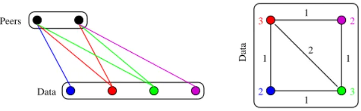
A natural way to encode the gathered data is to define a bipartite graph Q = (P, D, E), called query graph, as follows (see Figure 2, left):
Data 2 2 3 1 1 1 1 Data 2 3 Peers
Fig. 2.A query graph (left) and the associated (weighted) data graph (right).
– P is the set of peers in the network, D is the set of data,
– E⊆ P × D is a set of undirected edges, where {p, d} ∈ E if and only if the peer p is active for the data d, which means that p was interested for the data d or was a provider of d.
Notice that this graph evolves during time, and we will indeed consider it at various dates.
In order to analyze our data, we will also consider the (weighted) data graph D = (D, E, w) obtained from the query graph Q as follows (see Figure 2, right):
– D is the set of data,
– E ⊆ D × D is a set of undirected edges, where {d1, d2} ∈ E if and only if
there exists a peer active for both d1 and d2 in Q,
– wis a weight function over the nodes and the edges such that w(d) is the num-ber of data having been exchanged by peers active for d in Q and w(d1, d2)
is the number of data exchanged by peers in both d1 and d2in Q.
The sizes of query graphs and data graphs obtained from a typical trace at various times are given in Figure 1. We use these graphs, which have properties representative of what we observed of this kind of graphs, throughout this paper. In the following, we use these graphs and tools from the recent field of com-plex network analysis to deepen the study of the dynamic traces. We focus in particular on the data clustering, which captures how much the exchanges pro-cessed by two sets of peers are similar. In other words, it is a measure of how much peers active for at least one common data will exchange the same other data. We then show that these properties have significant impact on the effi-ciency of searches in the network, and therefore may be used in the design of efficient P2P protocols. Finally, we will use this analysis to study the relevance of a previously proposed model.
2
Data clustering analysis
Our aim now is to analyze similarities between data in terms of exchanges pro-cessed by peers active for them. In particular, given two data u and v exchanged
by a given peer p we are interested in the number of other common data ex-changed by peers actives for u or v. This can be measured using the following parameter over the edges in D:
c(u, v) = w(u, v) w(u) + w(v) − w(u, v)
Indeed, the two data u and v induce an edge {u, v} in D, the weight w(u, v) is nothing but the number of common data exchanged by peers active for u or v, and the expression w(u) + w(v) − w(u, v) gives the total number of data exchanged by peers active for u or v. Finally, c(u, v) therefore measures how much these exchanges overlap. Notice that its value is between 0 and 1.
The value of c(u, v) may however be strongly biased if one of the two nodes has a high weight and the other a low one: the value would then be very low. For example, if a data with an high popularity3
is connected to an unpopular one, then the clustering will probably be low, even if the few data exchanged by the lowest population are completely included in the large set of data exchanged by the highest one.
In order to capture these cases, we will also consider the following statistical parameter:
¯
c(u, v) = w(u, v) min(w(u), w(v))
which is still in [0; 1] but is always larger than c(u, v) and does not have this drawback. For instance, in the case described above the obtained value is 1.
We will call c(u, v) the clustering of {u, v} and ¯c(u, v) its min-clustering. In summary, the clustering captures the overlap between data exchanged by two sets of peers with no consideration of the heterogeneity between the number of data exchanged, whereas min-clustering takes into account and captures particularly well the fact that a small set of exchanged data can actually be a subset of a another much larger one.
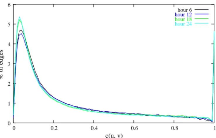
Figure 3 and 4 show the time-evolution of the distributions4
of c(u, v) and ¯
c(u, v), respectively. First notice that the general shape of these distributions is very stable along time, which indicates that the observations we will derive are not biased by the timescale or date considered.
Now let us observe (Figure 3) that around 60% of the edges always have a clustering lower than 0.2. This may indicate that the overlap of exchanges is not as high as expected. However, this may be a consequence of the fact that both the peer activity and the data popularity are very heterogeneous: there are very active peers while most of them are not, and there are very popular data
3
The popularity of a data is the number of peers active for that data.
4
The distribution of a parameter x is, for each possible value of x, the ratio between the number of instances of this value and the total number of instances. Here we will directly plot the number of instances of each value, which makes it possible to visualize traces of various sizes (i.e. at various dates) in a same plot.
% of edges c(u, v) 0 1 2 3 4 5 6 0 0.2 0.4 0.6 0.8 1 hour 6 hour 12 hour 18 hour 24
Fig. 3.Time evolution of the c(u, v) distribution
c(u, v) % of edges 0 5 10 15 20 25 30 0 0.2 0.4 0.6 0.8 1 hour 6 hour 12 hour 18 hour 24
Fig. 4.Time evolution of the ¯c(u, v) distribution
while most are not. This induces in D many links between data of very different popularity and a low clustering.
This can be corrected using the distribution of min-clustering (Figure 4): only 15% of the edges have a min-clustering lower than 0.2 while for nearly 60% higher or equal to 0.5. This indicates that the overlap is indeed high; for instance, 30% of the overlaps between all exchanges actually are a complete inclusion.
Such results may indicate the presence of a hierarchy among exchanges: while few popular data form the core of D, a large number of less popular ones have their exchanges mostly included into the ones of the core. If this structure indeed exists, it may be used to dynamicaly build a multicast tree from a P2P overlay.
We will discuss the presence of such a hierarchy and its implications later in this contribution.
3
Consequences on searching
Following several previous works (e.g. [3,6,13,14]), one may wonder if the prop-erties highlighted in previous section may be used to improve search in P2P systems. To answer this question, we will process the following experiment. We suppose that each peer has a knowledge of the peers active for the same data as itself. Then, when a peer p sends a query for a data d, it first looks at the other peers already active for a data p is active for. If one of them provides d, then it sends it directly to p. In this case, the clustering has been used and the data was found using only one hop search.
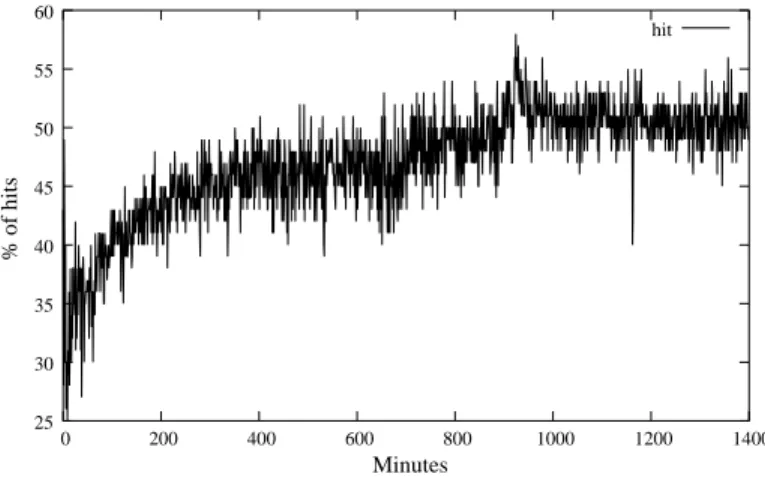
The time-evolution of this hit ratio is plotted in Figure 5. Despite it is quite low in the first few minutes (due to the server bootstrap), the ratio quickly converges to a value close to 50%.
Minutes % of hits 25 30 35 40 45 50 55 60 0 200 400 600 800 1000 1200 1400 hit
Fig. 5.Time evolution of the hit % using the one hop protocol
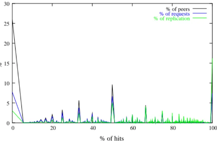
To deepen our understanding of what happens, let us consider Figure 6, in which we plotted the percentage of all the peers, the percentage of all the queries, and the replication of each data5
corresponding to the percentage of hits using a one hop search.
The first thing to notice is that nearly 25% of the peers do not find any data using the proposed approach. This is quite surprising, since we observed in Figure 5 that 50% of all the queries are routed with success using the same approach. This can be understood by observing that this ’null hit’ population generated only 7% of the queries and so only slighly influenced the high hit
5
% % of hits 0 5 10 15 20 25 30 0 20 40 60 80 100 % of peers % of requests % of replication
Fig. 6.Correlation between the % of peers, the associated % of queries they generated, the % of replication of the queried data and the % of hits they obtained after 24h using the one hop protocol
rate previously observed. Additionally, the queried data appear to be very rare at the time they were asked. This low volume of queries together with the low replication explain the null hit rate; these peers are not active for enough data nor enough replicated ones to find them using the one hop search.
On the other hand, more than 10% of the peers have a perfect success rate. One could think that such a result would imply a prohibitive amount of queries; Figure 6 indicates that it is not the case: the percentage of queries is close to the number of peers who processed them. Notice however that data found this way appear to be highly replicated (the population being active for these data at the time they were asked represents 15% of the peers active for other queried data) which explains the high success rate. Finally, notice that the average peer’s success rate increases from 40% to nearly 60% if the ’null hit’ population is removed from the calculus.
4
Modeling peer and data clusters
In [14] the authors propose a model to represent the semantic structure of P2P file sharing networks and use it to improve searching. They assume the existence of semantic types labelled by n ∈ {1, . . . , N } with N denoting the number of such types. They assume that each data and each peer in the system has exactly one type. A data of type n is called a n-data, and a peer of type n is called a n-peer. They denote respectively by dn and un the number of n-data and the
number of n-peer (u for user).
They denote by pn(m) the probability that a query sent by a n-user is for a
Clearly, a classification of peers and users captures clustering if, for all n and m, either pn(m) is close to 0 (n-peers almost never seek m-data) or it is quite
large (n-peers often seek m-data). If it is either 0 or 1 then the clustering is perfect: n-peers only seek m-data for that value of m such that pn(m) = 1.
This formalism is useful in helping to consider the hierarchical organisation induced by clustering, for the purpose of simulations for instance. We will see here that the statistical properties observed in previous section may be used to compute clusters of data, which make it possible to validate the model describe above. Moreover, we will give some information on parameters which may be used with the model to make its use realistic.
Cluster computation
Notice that computation of relevant clusters in general is a challenging task, computationaly extensive and untractable in practice on large graphs such as the one we consider. We can however propose a simple procedure based on the statistical properties of D observed in previous section: for two given integers 1 < ⊥ < ⊤ < |D|,
– sort edges by increasing values of their clustering – for each edge taken in this order:
• if its removal does not induce a connected component with less than ⊥ vertices then remove it
• if the size of the largest connected component if lower than ⊤ then terminate
We define the data clusters as the connected components finally obtained. The integers ⊥ and ⊤ are respectively the minimal and the maximal sizes of these clusters.
The idea behind this cluster definition is that edges between data of different clusters should have a low clustering, indicating that the clusters put together data with similar sets of exchanges.
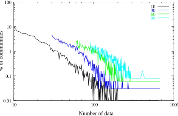
In our case, we observed that ⊤ = 1000 and ⊥ = 10 give good results, and that changing their values does not change significantly the results. We will illustrate this in the following by using ⊤ = 1000 and ⊥ ∈ {10, 30, 60, 90}. Notice that these values ensure both that the clusters will not be too small (they contain at least ⊥ data) and not too large (their size is bounded by ⊤).
Cluster properties
Figure 7 shows that the size distribution of clusters, i.e. the distribution of dn, is
well fitted by a power law (for all considered ⊥). Notice however that the average clusters sizes are highly influenced by ⊥, for instance, for ⊥ ∈ {10, 30, 60, 90}, the average clusters sizes are 30, 60, 100 and 150 respectively. There is indeed a natural correlation between ⊥ and the average size of clusters since, despite some contain up to 1 000 data, most clusters are small, with size close to ⊥. This
indicates that, when using the model proposed in [14], one may suppose a power law distribution for dn.
Let us now associate to each data cluster all the peers active for a data in the cluster. The number of peers associated this way is the popularity of the cluster. One may expect that these popularities will vary much, and that large clusters will be very popular, possibly concerning almost all the peers in the system.
Number of data % of communities 0.01 0.1 1 10 100 10 100 1000 10 30 90 60
Fig. 7.Distribution of the number of data per cluster for ⊥ ∈ {10, 30, 60, 90}
Figure 8 shows that this is not the case: very few clusters have a low popular-ity, and none has a huge popularpopular-ity, the maximum being lower than 4, 000 peers (to be compared to the total number of peers in the system, around 50, 000).
% of communities Number of peers 0.01 0.1 1 10 1 10 100 1000 10000 10 30 60 90
These statistics show that the clusters we defined, despite their simplicity, do capture non-trivial information concerning the peers. This might indicate that data clusters also define peer clusters, as assumed in [14].
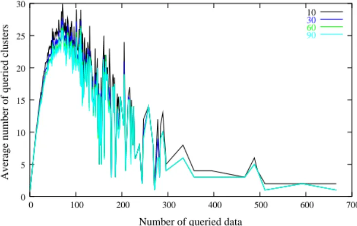
In order to check this, we plot in Figure 9 the correlations between the number of data peers are active for, and the average number of clusters this population queried in. This plot displays almost linear correlations until peers reach a degree 100 in D, but the correlation seems to be inverted after this limit: the most active peers queried data in very few clusters.
Average number of queried clusters
Number of queried data
0 5 10 15 20 25 30 0 100 200 300 400 500 600 700 10 30 60 90
Fig. 9. Correlation between the number of data queried and the average number of queried cluster for ⊥ ∈ {10, 30, 60, 90}
Several important observations can be done here. First, most of the peers do not ask for data in a constant number of clusters but rather in a number of clusters which depends on the number of queries they processed. In other words, peers do not ask for data in only one well identified cluster, in contradiction with what is assumed in [14].
This could make us conclude that, either the model should be improved to take this diversity into account, or a more subtle definition of clusters is necessary. Indeed, there are many ways in which data can be put into clusters, and the very simple one we proposed capture some features, but not all, of data/peers relations.
Notice that the previous plots do not capture the fact that a peer generally asks for many data in the same cluster (they only show that they ask for data in many clusters). This is exactly what pn(m), the ratio of m-data asked for by
n-peers, represents.
For each peer, we therefore have taken different values of pn(m) and see how
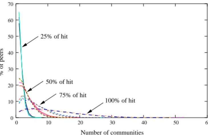
many clusters have to be queried by this peer to reach each of these values. We obtained this way the distributions of pn(m) plotted in Figure 10.
100% of hit 50% of hit 75% of hit 25% of hit % of peers Number of communities 0 10 20 30 40 50 60 70 0 10 20 30 40 50 60
Fig. 10.Number of clusters which has to be queried to get pn(m) = 25%, 50%, 75%
and 100% for ⊥ ∈ {10, 30, 60, 90}
It appears that approximately 60% of the peers can find 25% of the data they look for in only one cluster. This percentage of peers goes over 95% when we consider up to 3 clusters. Using the same procedure, we can see that asking only 5 clusters permits to 80% of the peers to find 50% of the data they look for. Likewise, considering still 5 clusters permits to more than 50% of the peers to find 75% of the data they look for.
Finally, this analysis shows that our simple cluster definition is enough to argue that the model proposed in [14] is relevant concerning the data and may be used with power law distributions of the size of clusters. It however shows that, despite non-trivial correlations are captured, either the cluster definition or the model fails in capturing a strict equivalence between a peer and a cluster. It rather indicates that most of the peers ask their data from a small set clusters, and not only one.
5
Conclusion
In this contribution, we proposed simple statistical parameters to capture the correlations between the set of peers active for a given data. We used these parameters first to confirm the previously noticed fact that semantic clustering can be used to improve search algorithms. Second, we used them to define a very simple and efficient way to compute data clusters. We have shown that these clusters succeed in capturing similarities between data.
We used these clusters to discuss the validity of a model of data clustering proposed in [14]. We obtained information on realistic parameters which should be used with this model. We also shown that the clusters we define can not be used directly with this simple model, which indicates that either a more subtle
cluster definition should be considered, or that the model should be extended. We pointed out some direction for this.
Notice that we focused here on data, but the same kind of approach may be fruitful with peers. A combination of the clusters we defined on data and clusters defined in a similar way on peers would probably bring significant improvement. More subtle cluster computations would also probably help, but we must keep in mind the huge size of the trace, which forbids intricate methods.
Finally, let us insist on the fact that the analysis of large real-world traces like the one we presented here is only at its beginning, and that much remains to understand from it. The lack of relevant statistical parameters (concerning for example the dynamics of the trace), and of efficient algorithms to deal with such traces are among the main bottleneck to this, but studies like the one we presented here show that simple methods can already bring much information.
References
1. E. Adar and B. Huberman. Free riding on gnutella, 2000.
2. Stevens Le Blond, Matthieu Latapy, and Jean-Loup Guillaume. Statistical analysis of a p2p query graph based on degrees and their time evolution. IWDC’04, 2004. 3. F. Le Fessant, S. Handurukande, A.-M. Kermarrec, and L. Massouli´e. Clustering in peer-to-peer file sharing workloads. 3rd International Workshop on Peer-to-Peer Systems (IPTPS), September 2004.
4. Jean-Loup Guillaume and Stevens Le Blond. P2p exchange network: Measurement and analysis. 2004.
5. Jean-Loup Guillaume and Stevens Le Blond. Statistical properties of exchanges in p2p systems. Technical report, PDPTA’04, 2004.
6. S. Handurukande, A.-M. Kermarrec, F. Le Fessant, and L. Massouli´e. Exploiting semantic clustering in the edonkey p2p network. 11th ACM SIGOPS European Workshop (SIGOPS), September 2004.
7. Nathaniel Leibowitz, Aviv Bergman, Roy Ben-Shaul, and Aviv Shavit. Are file swapping networks cacheable? characterizing p2p traffic. 7th International Work-shop on Web Content Caching and Distribution (WCW), August 2002.
8. Nathaniel Leibowitz, Matei Ripeanu, and Adam Wierzbicki. Deconstructing the kazaa network. The Third IEEE Workshop on Internet Applications, June 2003. 9. Jian Liang, Rakesh Kumar, and Keith Ross. Understanding kazza, 2004. 10. Lugdunum. lugdunum2k.free.fr/.
11. S. Saroiu, K. Gummadi, R. Dunn, S. Gribble, and H. Levy. An analysis of internet content delivery systems, 2002.
12. Subhabrata Sen and Jia Wang. Analyzing peer-to-peer traffic across large networks. Internet Measurement Workshop 2002, November 2002.
13. K. Sripanidkulchai, B. Maggs, and H. Zhang. Efficient content location using interest-based locality in peer-to-peer systems. Internet Measurement Workshop 2002, November 2002.
14. S. Voulgaris, A.-M. Kermarrec, L. Massoulie, and M. van Steen. Exploiting se-mantic proximity in peer-to-peer content searching. 10th IEEE Int’l Workshop on Future Trends in Distributed Computing Systems (FTDCS), May 2004.
15. rfc-gnutella.sourceforge.net/developer/testing/index.html www.bittorrent www.kazaa.com, www.edonkey2000.com.