HAL Id: hal-00295359
https://hal.archives-ouvertes.fr/hal-00295359
Submitted on 12 Nov 2003
HAL is a multi-disciplinary open access
archive for the deposit and dissemination of
sci-entific research documents, whether they are
pub-lished or not. The documents may come from
teaching and research institutions in France or
abroad, or from public or private research centers.
L’archive ouverte pluridisciplinaire HAL, est
destinée au dépôt et à la diffusion de documents
scientifiques de niveau recherche, publiés ou non,
émanant des établissements d’enseignement et de
recherche français ou étrangers, des laboratoires
publics ou privés.
stratospheric dynamical and chemical processes in a
coupled chemistry-climate model
D. Lamago, M. Dameris, C. Schnadt, V. Eyring, C. Brühl
To cite this version:
D. Lamago, M. Dameris, C. Schnadt, V. Eyring, C. Brühl. Impact of large solar zenith angles on lower
stratospheric dynamical and chemical processes in a coupled chemistry-climate model. Atmospheric
Chemistry and Physics, European Geosciences Union, 2003, 3 (6), pp.1981-1990. �hal-00295359�
Atmos. Chem. Phys., 3, 1981–1990, 2003
www.atmos-chem-phys.org/acp/3/1981/
Atmospheric
Chemistry
and Physics
Impact of large solar zenith angles on lower stratospheric dynamical
and chemical processes in a coupled chemistry-climate model
D. Lamago1,∗, M. Dameris1, C. Schnadt1, V. Eyring1, and C. Br ¨uhl2
1Institut f¨ur Physik der Atmosph¨are, DLR-Oberpfaffenhofen, D-82234 Wessling, Germany 2Max-Planck-Institut f¨ur Chemie, D-55020 Mainz, Germany
∗
now at: ZWE FRM-II and Institut f¨ur Experimentalphysik E21, TU-M¨unchen, D-85748 Garching, Germany Received: 4 June 2003 – Published in Atmos. Chem. Phys. Discuss.: 22 July 2003
Revised: 25 October 2003 – Accepted: 29 October 2003 – Published: 12 November 2003
Abstract. Actinic fluxes at large solar zenith angles (SZAs)
are important for atmospheric chemistry, especially under twilight conditions in polar winter and spring. The results of a sensitivity experiment employing the fully coupled 3D chemistry-climate model ECHAM4.L39(DLR)/CHEM have been analysed to quantify the impact of SZAs larger than 87.5◦ on dynamical and chemical processes in the lower stratosphere, in particular their influence on the ozone layer. Although the actinic fluxes at SZAs larger than 87.5◦are small, ozone concentrations are significantly affected be-cause daytime photolytic ozone destruction is switched on earlier, especially at the end of polar night the conversion of Cl2and Cl2O2into ClO in the lower stratosphere.
Compar-ing climatological mean ozone column values of a simula-tion considering SZAs up to 93◦with those of the sensitivity
run with SZAs confined to 87.5◦total ozone is reduced by about 20% in the polar Southern Hemisphere, i.e., the ozone hole is “deeper” if twilight conditions are considered in the model because there is about 4 weeks more time for ozone destruction. This causes an additional cooling of the polar lower stratosphere (50 hPa) up to −4 K with obvious con-sequences for chemical processes. In the Northern Hemi-sphere the impact of large SZAs cannot be determined on the basis of climatological mean values due to the pronounced dynamic variability of the stratosphere in winter and spring. This study clearly shows the necessity of considering large SZAs for the calculation of photolysis rates in atmospheric models.
1 Introduction
Chemistry-climate links have received increased attention in recent years (IPCC, 2001; EC, 2003; WMO, 2003). The
in-Correspondence to: M. Dameris
(Martin.Dameris@dlr.de)
vestigation of mutual effects of dynamical, chemical, and ra-diative coupling in the Earth’s atmosphere is currently an out-standing scientific issue. Improved knowledge is necessary to better understand the relations between changes in atmo-spheric composition and climate. One key question, for ex-ample, is to which extent the recent destruction of the ozone layer has been affected by radiative cooling of the strato-sphere due to increased greenhouse gas concentrations and how this will influence future ozone recovery.
Fully coupled three-dimensional (3D) chemistry-climate models (CCMs) are suitable tools to investigate the impor-tance of these mutual effects. CCMs have been used to sim-ulate the recent and future development of the chemical com-position and the dynamics of the atmosphere (e.g. Rozanov et al., 2001; Austin, 2002; Schnadt et al., 2002; Nagashima et al., 2002; Pitari et al., 2002; Steil et al., 2003). The un-certainties and assessments of the currently available CCMs have been recently summarised by Austin et al. (2003).
In this study the CCM ECHAM4.L39(DLR)/CHEM (hereafter E39/C) is employed to assess the impact of so-lar zenith angles (SZAs) so-larger than 87.5◦for the chemistry and dynamics of the lower stratosphere, in particular at polar latitudes during winter and spring. It is well-known that the impact of photolysis on mixing ratios of chemical species depends on the maximum SZA allowed in model calcula-tions. For example, an estimate by the 2D chemistry model MPIC for a specific case study at the 475 K isentropic level showed that the relative total ozone loss increased from 25% to 31% when the maximum SZA was raised from 90◦to 92◦
(Kr¨amer et al., 2003). Moldanova et al. (2002) showed that for some halogenated species and NO3, the photolysis
be-yond 90◦ SZA may be of importance. Nevertheless, most CCMs neglect the impact of twilight for simplicity reasons, which certainly has an impact on chemical processes, espe-cially during winter and spring near the edge of the polar night.
This paper aims to quantify the effect of photolysis beyond 87.5◦SZA in a fully coupled 3D CCM. In the next section
the employed model system E39/C is briefly described, with special focus on the parameterisation of the photolysis up to 93◦SZA used here. The numerical simulations forming the basis for this investigation are briefly introduced. In Sect. 3 the model results are discussed, i.e., changes of photolysis frequencies, of ozone mixing ratios, and of related dynamical and chemical effects. Our conclusions are presented in the last section.
2 Model description and design of experiments
2.1 Brief description of E39/C
In this study the interactively coupled chemistry-climate model E39/C is employed. More detailed descriptions of the model are given in Hein et al. (2001) and Schnadt et al. (2002). The model horizontal resolution is T30. In the ver-tical, E39/C has 39 layers from the surface to the top layer centred at 10 hPa (Land et al., 2002). The chemistry mod-ule CHEM (Steil et al., 1998) is based on the family con-cept. It describes relevant stratospheric and tropospheric O3
related homogeneous chemical reactions and heterogeneous chemistry on polar stratospheric clouds (PSCs) and sulphate aerosols, it does not consider bromine chemistry. E39/C in-cludes an online feedback of chemistry, dynamics, and ra-diative processes. Chemical tracers are advected by the sim-ulated winds. The net heating rates, in turn, are calcsim-ulated us-ing the actual 3D distributions of the radiatively active gases O3, CH4, N2O, H2O, and CFCs. Climatological means of
dynamical and chemical fields have been intensively vali-dated with regards to other model results and to observations (e.g., Austin et al., 2003; Land et al., 2002; Hein et al., 2001). 2.2 Parameterisation of photolysis frequencies at large
SZAs
The photolysis frequencies for SZAs less equal 87.5◦are cal-culated using the efficient method of Landgraf and Crutzen (1998) (see also Landgraf, 1998). The spectral range (178.6 nm ≤λ≤ 752.5 nm) relevant for the photo-chemistry of the troposphere and the middle atmosphere is divided into 8 wavelength intervals Ii(i =1, ..., 8). For each interval, the
photolysis frequency Ji,x of a gas x is calculated according
to the equation: Ji,x =
Z
Ii
σx(λ)8x(λ)F (λ)dλ, (1)
where σx(λ)is the absorption cross section, 8x(λ)the
quan-tum yield, and F (λ) the actinic flux in the interval Ii. In
the spectral range of 202.0 nm ≤λ≤ 752.5 nm, scattering at air molecules, aerosols, and clouds is not negligible. To include this efficiently, Ji,xis calculated from precalculated
photolysis frequencies for a purely absorbing atmosphere us-ing Eq. (1) with high spectral resolution and a correction fac-tor for the scattering effects:
Ji,x=Ji,xa δi (2) with δi = F (λi) Fa(λ i) . (3)
Fa(λi) and Fa(λ) (see Eq. 4) are the actinic fluxes for a
purely absorbing atmosphere for the wavelength λi and λ in
the interval Ii. They are calculated using the Lambert-Beer
absorption law: Fa(λ) = F0(λ)exp{−
X
k
Vkσk(λ)}, (4)
where F0(λ)is the spectral solar irradiance at the model top,
Vk is the slant column, and σk is the absorbtion cross
sec-tion of the kth absorber (O2and O3). The correction factor
δi is calculated online with a radiative transfer code
(Zdun-dowski et al., 1980) at λi of Landgraf and Crutzen (1998).
It takes into account scattering as well as absorption due to air molecules, aerosols, clouds, and the Earth’s surface albedo. The photolysis frequency is determined by the fol-lowing equation: Jx≈J1,xa + 8 X i=2 Ji,xa δi. (5)
Here, J1,xa is the photolysis frequency in the spectral range of the Schumann-Runge band (178.6 nm≤λ≤202.0 nm), where O2 is a strong absorber and scattering can be
ne-glected. So far, Ji,xa is calculated for an isothermal atmo-sphere. To account for the temperature dependence of σ and 8, a correction function is applied. For further details of the parametrisation of Ji,xa and the temperature dependence see Landgraf (1998). Equations (1) to (5) are valid for SZAs up to 87.5◦. For larger SZAs, the parameterisation of photolysis frequencies is done according to the laws of spherical geom-etry, where the actinic flux for a given wavelength depends on the SZA θ (Levy II, 1974). R¨oth (1992, 2002) introduced the following empirical formula for photolysis frequencies which includes very large zenith angles:
J = J0·exp[b(1 − sec(cθ ))], (6)
with J0photolysis frequency for overhead sun and standard
atmosphere at a certain altitude and empirical coefficients b and c which are tabulated for all species of interest. In E39/C we use a simplified version of this fit only for SZAs larger 87.5◦. To account for the interactively calculated at-mospheric quantities like ozone columns and reflection from clouds we adopt the J-value at SZA 87.5◦, obtained with the
Landgraf and Crutzen (1998) scheme and multiply that with a correction formular derived from Eq. (6):
Lamago et al.: Impact of twilight in a CCM 1983
Table 1. The coefficients bi of Eq. (7) for the different species
(channels), grouped by wavelength region most important for pho-tolysis.
bi species region
1 O3(→O(3P)), NO2, NO3 UV-A or visible
1.3 ClONO2, Cl2O2 UV-A
1.4 HOCl near UV-B
1.5 CH2O(M), N2O5, HNO4, CH3O2H UV-B
2 CH2O(R), H2O2 UV-B 3 O3(→O(1D)) far UV-B
4 HNO3 far UV-B
5 O2, CFC-11, CFC-12, CCl4, CH3Cl, CH3CCl3, HCl, H2O, CO2, N2O, NO UV-C with Fcorr =exp[19.09bi(1 − θ 87.5)]. (8)
The empirical coefficients bi in Eq. (8) are species
depen-dent and listed in Table 1. They are derived from the ratio of Eq. (6) evaluated at θ equal 93◦and 87.5◦(with F
corr=1
for θ =87.5◦). For SZAs larger 93◦ night is assumed. This simplification can be justified because for polar stratospheric conditions mostly the on/off effect at sunrise/sunset matters. For SZAs between about 70◦and 87.5◦for the airmass fac-tor d(θ ) used in the photolysis calculation in Landgraf and Crutzen (1998) an empirical correction for the curvature of the atmosphere based on the Chapman-function is addition-ally applied (e.g. Lacis and Hansen, 1974):
d(θ ) =√ 35
1224 cos2θ +1. (9)
For smaller SZAs d(θ ) converges to 1/ cos θ . This technique allows to calculate the photolysis rates online in a realistic atmospheric state, in which the SZA is time dependent. 2.3 Model experiments
Two timeslices representing atmospheric conditions for the early 1990s have been used, namely, a control scenario in-cluding SZAs up to 93◦(SZA93) and a sensitivity simulation which does not consider SZAs larger than 87.5◦(SZA87.5) (see Sect. 2.2). Each timeslice has been integrated over 24 years under steady state conditions with the first four years taken as spin-up. For both model simulations, climatologi-cal mean sea surface temperatures (SST) are prescribed from observations for the years 1979 to 1994 (Gates, 1992). In ad-dition, natural and anthropogenic NOxemissions are fixed at
the surface. At the model top, mixing ratios of NOyand ClX
(=ClOx+ClONO2+HCl) are prescribed to account for higher
altitude chemistry above the upper boundary. Moreover, the global mean values of the mixing ratios for the most relevant greenhouse gases CO2, CH4, and N2O are fixed at the lower
Table 2. Mixing ratios of greenhouse gases, inorganic chlorine,
and NOxemissions of different natural and anthropogenic sources
for the “1990” simulations (i.e., the SZA87.5 and the SZA93 run, respectively). CO2(ppmv) 353 CH4(ppmv) 1.69 N2O (ppbv) 310 Cly(ppbv) 3.4 NOxlightning (Tg(N)/year) 5.3
NOxair traffic (Tg(N)/year) 0.6
NOxsurface (total) (Tg(N)/year) 33.1
NOxsurface (industry, traffic) 22.6
NOxsurface (soils) 5.5
NOxsurface (biomass burning) 5.0
boundary for each scenario (Hein et al., 2001). They are specified according to observations for the year 1990. The specific boundary conditions are summarised in Table 2.
3 Discussion of results
3.1 Changes of photolysis frequencies
Neglecting large SZAs is associated with less photons at the day-night transition and in particular with a delay of daytime chemistry at the end of the polar night with significant effects for the destruction of ozone in the polar lower stratosphere. The photolysis of heterogeneously formed Cl2at large SZAs
after polar night initiates the catalytic ozone destruction by chlorine. Ozone depletion rates are highly related to the pho-tolyis rates of Cl2O2(→O2+2Cl).
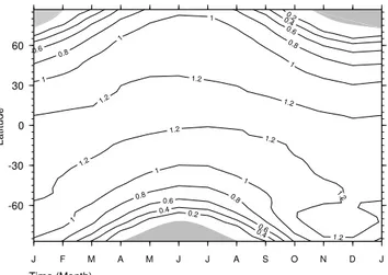
Figure 1 shows the absolute values of the photolysis fre-quencies of Cl2O2for a single model year at 50 hPa of the
simulation SZA93. The structure of this field obviously re-flects the importance of ozone as the dominant absorber: the photolysis frequencies are enhanced southward of 60◦S between October and November (more than 1.2·10−3 s−1), when ozone column values are still small and actinic fluxes differ significantly from zero. Including SZAs larger than 87.5◦leads to changes in the photolysis frequencies of Cl
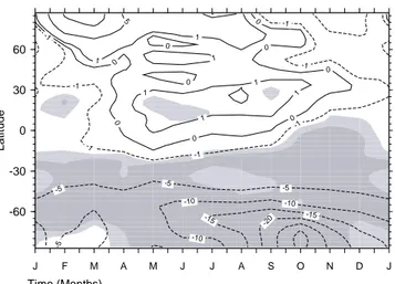
2O2
as is displayed in Fig. 2 for the 50 hPa level. As expected, the most obvious changes are detected at the edge of the polar night (up to 0.6·10−4s−1) in both hemispheres. In the South-ern Hemisphere absolute differences of the same order of magnitude are found in the polar region at the end of Novem-ber, and correspond to about 5%. The maximum changes in November are indirectly produced by reduced ozone in SZA93 (see Sect. 3.2).
0.2 0.2 0.4 0.4 0.4 0.6 0.6 0.6 0.6 0.8 0.8 0.8 0.8 1 1 1 1 1 1 1 1.2 1.2 1.2 1.2 1.2 1.2 1.2 1.2 -60 -30 0 30 60 Latitude J F M A M J J A S O N D J Time (Month)
Fig. 1. Photolysis frequencies (noon values) of Cl2O2[10−3s−1]
at 50 hPa in SZA93. Shaded areas indicate polar night, i.e., photo-lysis frequencies are zero. Letters at the x-axis denote the beginning months.
3.2 Change of ozone 3.2.1 Ozone columns
In order to evaluate the impact of twilight on upper tropo-spheric and lower stratotropo-spheric chemistry, we first compare the results of the climatological mean total ozone averaged over 20 simulated years including solar zenith angles up to 93◦(SZA93) (Fig. 3) to the values of a simulation that only considered SZAs up to 87.5◦(SZA87.5) (Fig. 4). A detailed comparison of the results presented in Figure 4 with obser-vations (Bojkov et al., 1999) was presented in Hein et al. (2001). There, it was concluded that in the tropics as well as in the northern extra-tropics, the seasonal variations of sim-ulated total ozone are in agreement with measurements, al-though the absolute total ozone values are overestimated by about 25 DU. In the southern extra-tropics, simulated ozone values are close to observations, but the seasonal variabil-ity of total ozone shows some noticeable differences. For example, the midlatitude modelled Austral spring maximum occurs earlier than observed (about 1 month) and the ozone hole season (i.e., total ozone locally less than 220 DU) lasts longer (i.e., until the beginning of December instead of end of October).
Figure 5 shows the differences between the modelled cli-matological mean total ozone fields (SZA93-SZA87.5). In the southern mid- and high latitudes between 30◦S and 90◦S
the largest ozone difference values are simulated. These dif-ferences are statistically significant due to the relative low inter-annual variability. The ozone reduction is strongest south of 60◦S between September and November due to the photon surplus in SZA93. The maximum differences are found in the centre of the polar vortex. At the end of September approximately 30 Dobson Units (DU) less ozone
0.2 0.2 0.2 0.2 0.2 0.2 0.2 0.2 0.2 0.4 0.4 0.4 0.4 0.6 -0.2 -0.2 -90 -60 -30 0 30 60 90 Latitude J F M A M J J A S O N D J Time (Month)
Fig. 2. Differences in photolysis frequencies (noon values)
of Cl2O2 [10−4 s−1] at 50 hPa between SZA93 (Fig. 1) and
SZA87.5. Positive differences indicate higher photolysis frequen-cies in SZA93.
are found in the SZA93 case. This corresponds to a max-imum reduction of the ozone column over the south polar region of about 20% in the SZA93 run in comparison to the SZA87.5 simulation. A closer inspection indicates that in the SZA93 simulation ozone depletion starts earlier. Figure 6 shows the temporal development of total ozone at 70◦S and 83◦S. For example, contemplating the 83◦S curve, the ozone hole season appears 3 weeks earlier in SZA93 (i.e., first de-tection of total ozone values less than 220 DU) than in the SZA87.5 run and the minimum value is reached five days earlier. Both findings are an improvement with respect to ob-servations. The lifetime of the ozone hole is about ten days longer in the SZA93 simulation. The latter result exhibits a slight degradation of model results with regards to the obser-vations mentioned above. Similar changes are found at 70◦S,
however the minimum values in SZA87.5 do not fall below 230 DU.
The statistically significant change of total ozone at South-ern Hemisphere midlatitudes (about 20◦S to 50◦S) cannot be directly due to ClO-dimer photolysis. The main reason is additional ozone destruction by NOxcatalysis in SZA93
(due to enhanced photolysis of N2O5at a longer day), which
is important in the altitude range between 10 and 100 hPa in mid- and high latitudes. For example, in midlatitudes of the Southern Hemisphere at 50 hPa NOxis enhanced by
be-tween 10 and 50 pptv in the SZA93 simulation, which is approximately 10% (not shown). Br¨uhl and Crutzen (2000) pointed out that although in summer net chemical ozone pro-duction occurs in the latitude region between the subtrop-ical barrier and about 50◦, total ozone declines in this re-gion because of exchange with the net chemical destruction regions (which are larger for the SZA93 case) in high lati-tudes and in the troposphere. Here, we can conclude that the
Lamago et al.: Impact of twilight in a CCM 1985 175 200 225 250 250 275 275 275 275 275 275 300 300 300 300 300 300 300 300 325 325 325 325 325 325 325 350 350 350 375 375 375 400 425 -60 -30 0 30 60 Latitude J F M A M J J A S O N D J Time (Months)
Fig. 3. Modelled climatological zonal mean total ozone (in Dobson
Units, DU) taking in account SZAs up to 93◦(SZA93). The model results are averaged over 20 simulated years.
200 225 250275 275 275 300 300 300 300 300 300 300 300 300 325 325 325 325 325 325 325 350 350 350 350 375 375 400 425 -60 -30 0 30 60 Latitude J F M A M J J A S O N D J Time (Months)
Fig. 4. Same as in Fig. 5, but considering SZAs up to 87.5◦only
(SZA87.5).
Southern Hemisphere midlatitude total ozone values of the SZA93 simulation are in better agreement with observations than those of SZA87.5.
In high latitudes of the Northern Hemisphere total ozone is moderately increased by about 2% to 4% between Febru-ary and the middle of March. Due to the high inter-annual dynamic variability of the Northern Hemisphere polar strato-sphere, these changes are not statistically significant. This does not principally exclude that individual cold Northern Hemisphere model winters experience similar large SZA ef-fects as is generally found in the Southern Hemisphere. Sev-eral papers showed that photochemical box model calcula-tions cannot reproduce observed ozone loss rates during cold Arctic Januaries (e.g. Becker et al., 1998; Hansen and Chip-perfield, 1999; Rex et al., 2003). Although it seems that the missing ozone loss mechanism is important at large SZAs
0 0 0 0 0 0 0 0 0 1 1 1 1 1 1 1 5 -1 -1 -1 -1 -1 -1 -1 -5 -5 -5 -5 -10 -10 -10 -15 -15 -20 -60 -30 0 30 60 Latitude J F M A M J J A S O N D J Time (Months)
Fig. 5. Changes of total ozone (in DU) between SZA93 and
SZA87.5. Negative (positive) values indicate lower (higher) val-ues in SZA93. Dark (light) shaded areas indicate the 99% (95%) significance level (t-test).
Fig. 6. Temporal development of climatological zonal mean total
ozone columns (in DU) at 70◦S (top) and at 83◦S (bottom). Dashed (solid) lines denote results from the simulation SZA87.5 (SZA93).
and low temperatures, the discrepancies between the model results and observations cannot be solely explained due to the models restricting the photolysis calculations to SZAs of less than 90◦, at best it can explain a small part of it.
In tropical regions, as well as in midlatitudes of the North-ern Hemisphere only small changes occur due to larger SZAs. The differences in the tropics are about 1% (approx-imately 3 DU), they are partly statistically significant. This can be explained considering the mean ozone value of about 275 DU in the tropics and the very low inter-annual dynamic variability in these regions.
Pressure [hPa] 300 200 150 100 70 30 10 90˚S 60˚S 30˚S Equator 30˚N 60˚N 90˚N January 0 0 0 0 0 10 -10 -10 -10 -20 -20 -20 -50 -50 -50 -50 -100 Pressure [hPa] 300 200 150 100 70 30 10 90˚S 60˚S 30˚S Equator 30˚N 60˚N 90˚N April 0 0 0 10 10 20 20 -10 -10 -10 -20 -20 -20 -50 -50 Pressure [hPa] 300 200 150 100 70 30 10 90˚S 60˚S 30˚S Equator 30˚N 60˚N 90˚N July 0 0 0 0 10 10 10 10 20 20 -10 -10 -10 -20 -20 -20 -50 -100 Pressure [hPa] 300 200 150 100 70 30 10 90˚S 60˚S 30˚S Equator 30˚N 60˚N 90˚N October 0 0 0 0 10 10 10 -10 -10 -10 -20 -20 -20 -50 -50 -100 -200 latitude latitude latitude latitude
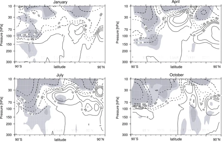
Fig. 7. Changes of climatological zonal mean ozone mixing ratios (ppbv) depending on altitude and latitude for January, April, July, and
October. Negative (positive) values indicate lower (higher) values in SZA93. Heavy (light) shaded areas indicate the 99% (95%) significance level (t-test). Isolines are plotted on a logarithmic scale: −500, −200, −100, −50, −20, −10, 0, 10, 20, 50, 100.
3.2.2 Zonal mean ozone difference
To investigate the modelled ozone changes due to large SZAs in more detail, differences of zonal mean ozone mixing ratios are presented in Fig. 7 showing changes for January, April, July, and October. Nearly no changes of ozone mixing ra-tios are calculated below 150 hPa, most of the differences occur in the stratosphere. Ozone mixing ratios significantly decrease during southern spring at levels between 100 hPa and the model top. In SZA93, additional ozone decreases are mainly detected inside the polar vortex (south of ∼65◦S). At the centre of the polar vortex, between 70 hPa and 10 hPa an ozone reduction of more than −500 ppbv is found in Octo-ber. As already noted, sun rays enter the model atmosphere region between 65◦S and the South pole earlier in spring in SZA93 than in SZA87.5. The photon surplus at the edge of the polar night is responsible for the increased ozone destruc-tion (see Sect. 3.1).
At midlatitudes and in the tropical regions, ozone de-creases are larger at the upper model levels than at lower levels. Ozone differences up to −50 ppbv are simulated in January between 60◦S and 10◦S and between 30 hPa and
10 hPa. Because of the ozone reduction at the upper model levels, more sunlight penetrates down to lower atmospheric layers which has an impact on dynamics (temperature) and chemistry. Ozone differences are small in the equatorial re-gions. In April and July, ozone concentrations are larger in SZA93 by about 20 ppbv in comparison to SZA87.5. This is probably due to a slightly distinct circulation pattern pro-ducing small differences in the climatological mean ozone distributions in both model experiments (Sect. 3.3).
The Arctic stratosphere shows some modifications in ozone mixing ratios, however, these changes are mostly not statistically significant due to the high dynamic inter-annual variability of the Northern Hemisphere. The described ozone changes caused by considering large SZAs are due to dynam-ical and chemdynam-ical effects. In the next two sections we will quantify some of these effects in E39/C.
3.3 Change of dynamics
Statistically significant temperature differences between the SZA93 and the SZA87.5 simulations are mainly found in the extra-tropical Southern Hemisphere lower stratosphere
Lamago et al.: Impact of twilight in a CCM 1987 0 0 0 0 0 0 0 0 0 0.5 0.5 0.5 1 -0.5 -0.5 -0.5 -0.5 -0.5 -0.5 -0.5 -0.5 -1 -1.5 -2 -60 -30 0 30 60 Latitude J F M A M J J A S O N D J Time (Months)
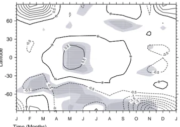
Fig. 8. Changes of climatological mean temperatures (K) at 50 hPa
between SZA93 and SZA87.5. Negative (positive) values indicate lower (higher) values in SZA93. Heavy (light) shaded areas indicate the 99% (95%) significance level (t-test).
(between 10 and 100 hPa). Figure 8 shows the differences for the 50 hPa pressure level. The largest values occur during po-lar spring (up to −4 K) indicating that the SZA93 simulation produces colder conditions there. Near the edge of the South-ern Hemisphere polar vortex the SZA93 run shows a cooling between −0.5 K and −1 K. These temperature differences can be easily related to the detected changes of the ozone column between the two model runs discussed in the last two sections (Fig. 5). In SZA93, the stratosphere is colder in re-gions with reduced ozone with regards to the SZA87.5 run. In the Northern Hemisphere, higher temperatures are found in the SZA93 case in later winter and early spring in the po-lar region due to the increase of ozone. As mentioned be-fore, these differences are statistically not significant due to the high dynamic inter-annual variability in this time of the year and region. Therefore, these temperature differences are fortuitous and cannot be interpreted. The increase of ozone in the tropics in the SZA93 run (i.e., about 2 DU in May and June) produces a warming of approximately 0.7 K. Although these differences are small they are statistically significant because the inter-annual variability in the equatorial region is very small.
The differences in the temperature fields result in cor-responding differences in the mean zonal wind fields (not shown). However, these are statistically not significant, nei-ther in the Sounei-thern nor in the Nornei-thern Hemisphere. For ex-ample, the Southern Hemisphere polar night jet is stronger in the SZA93 simulation by about 2 m/s. In the Northern Hemi-sphere, the wintertime stratospheric polar vortex is weaker (about −2 m/s) in SZA93. These results are consistent with the formerly discussed ozone and temperature differences.
Altogether it can be summarised that the mean climato-logical temperature conditions are clearly different in the
po-0.1 0.1 0.1 0.1 0.1 0.1 0.1 0.1 0.1 0.5 0.5 0.9 0.9 1 1.5 2 -80 -70 -60 -50 -40 -30 Equivalent latitude
Jul Aug Sep Oct Nov
Time (Months)
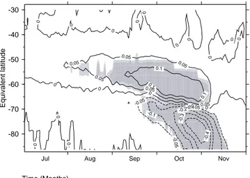
Fig. 9. Changes of the climatological zonal mean PSC I-NAT
(ppbv) at 50 hPa in the Southern Hemisphere between SZA93 and SZA87.5. Model data are transformed to the PV-coordinate sys-tem. Positive (negative) values indicate higher (lower) values in the SZA93 simulation. Heavy (light) shaded areas indicate the 99% (95%) significance level (t-test).
lar Southern Hemisphere. This has a strong impact on the temperature-dependent chemistry, in particular on the forma-tion of polar stratospheric clouds (PSCs) and thus on hetero-geneous ozone destruction (see Sect. 3.4).
3.4 Change of chemistry
To estimate the importance of considering SZAs larger than 87.5◦on stratospheric chemistry in a fully coupled 3D CCM, some chemical species have been analysed which are espe-cially relevant for polar chemistry. In the following, we con-centrate on Southern Hemisphere winter and spring condi-tions where the differences of climatological mean fields be-tween the two model simulations are most obvious. For an appropriate presentation of the results, a coordinate transfor-mation is carried out from the standard coordinate system to a description employing equivalent potential vorticity (PV) co-ordinates (e.g. Butchart and Remsberg, 1986; Manney et al., 1994). Here, the centre of the coordinate system is chosen to be the centre of the polar vortex. Isentropic contours are then used to define equivalent latitudes, for which ’zonal means’ with respect to the centre of the polar vortex are computed.
As shown in the previous section, stratospheric tempera-tures are reduced if SZAs up to 93◦are considered. Main
temperature differences between the SZA93 run and the SZA87.5 simulation are found in springtime inside the po-lar vortex. This favours the formation of PSCs in the SZA93 run. In this region the conditions are most favourable for het-erogenous chemistry on PSC surfaces during the polar night. Figures 9 and 10 show the differences of PSC I and II mix-ing ratios between the two simulations at 50 hPa. Obviously, a statistically significant increase of NAT and ice particles
50 50 50 50 50 50 50 50 100 100 150 150 -50 -50 -100 -80 -70 -60 -50 -40 -30 Equivalent latitude
Jul Aug Sep Oct Nov
Time (Months)
Fig. 10. As Fig. 9, but for PSC II-ICE (pptv).
can be found in SZA93 reflecting the differences in temper-atures. Both figures illustrate that the enhancement is firstly seen at the inner edge of the polar vortex in mid-winter. Max-imum differences are shifted towards higher latitudes with time with the size of the polar vortex becoming smaller.
The photon surplus increases the photolysis of chlorine compounds (Cl2O2, Cl2, HOCl, and ClONO2) in SZA93.
ClO and Cl radicals are released and enhance the destruc-tion of ozone through catalytic reacdestruc-tions, especially the so-called “dimer cycle” involving Cl2O2which is quadratic in
ClO. Figure 11 shows the differences in ClOxat the 50 hPa
pressure level. An enhanced activation of chlorine is found inside the polar vortex between July and November. Maxi-mum difference values are about 0.5 ppbv, these differences are statistically significant. An exception is found in the core region of the polar vortex in the second half of Octo-ber where a decrease of ClOx(up to −0.3 ppbv) is detetected
in the SZA93 run. This can be explained considering the re-lated differences of ClONO2and HCl which are displayed in
Figs. 12 and 13. Reduced ClONO2mixing ratios are found
in the SZA93 run inside the polar vortex between mid Oc-tober and mid November while HCl is increased there. This behaviour can be explained as follows: the chemical reac-tion Cl + O3→ClO + O2 determines the rate of formation
of ClONO2. Since in the model during this time only little
ozone (0.5 ppmv or less) is available, less chlorine monox-ide (ClO) is produced which can be transformed to ClONO2
(ClO + NO2+M→ClONO2+M). In case of low ozone
the ratio Cl/ClO is large leading to fast re-formation of the HCl reservoir (Cl + CH4→HCl + CH3). Thus, the chlorine
atoms formed by the photolysis of Cl2and Cl2O2after mid
October do not primarily react with ozone, but with methane which produce an increase of HCl. This model behaviour is in agreement with box model calculations and HALOE observations (Grooß et al., 1997; Steil et al., 2003). Al-though the results of both E39/C simulations show a
real-0 0 0 0 0 0 0.1 0.1 0.1 0.1 0.1 0.1 0.1 0.2 0.2 0.2 0.2 0.2 0.3 0.3 0.3 0.3 0.4 0.40.5 -80 -70 -60 -50 -40 -30 Equivalent latitude
Jul Aug Sep Oct Nov
Time (Months)
Fig. 11. As Fig. 9, but for ClOx(ppbv).
istic behaviour with regards to the re-formation of the chlo-rine reservoirs HCl and ClONO2, i.e., ClOxis first converted
towards HCl, the SZA93 simulation produces improved re-sults concerning the time of re-formation (2 weeks earlier), which means that they are closer to the analyses of observa-tions given by Grooß et al. (1997) and Steil et al. (2003). For completeness it is worthwhile mentioning that the collar of ClONO2is enhanced in the SZA93 simulation, as expected.
4 Conclusions
The current sensitivity study with the fully coupled CCM E39/C has shown that photolysis reactions during twilight have a non-negligible impact on the lower stratosphere, al-though the actinic fluxes for SZAs larger 87.5◦ are small. Considering climatological mean values, statistically signif-icant effects on the chemistry and dynamics of the lower stratosphere are mainly found in higher latitude regions of the Southern Hemisphere during winter and spring. Obvi-ous changes are also detected in midlatitudes of the South-ern Hemisphere which can be partially attributed to enhanced ozone destruction in the lower stratosphere by enhanced NOx
catalysis in the SZA93 simulation. Due to the high dynamic variability of the Northern Hemisphere lower and middle stratosphere, similar effects cannot be detected there. Cer-tainly, in individual cold Northern Hemisphere winter peri-ods with a stable polar vortex analogous results would be ob-tained. The detected changes of dynamic and chemical val-ues in the tropics and in midlatitudes of the Northern Hemi-sphere can be neglected.
In E39/C, the small surplus of photons for SZAs larger 87.5◦produces a different climatological mean ozone distri-bution. In the SZA93 run, ozone destruction is stronger, in particular in the southern extra-tropics. The maximum effect is found near the South Pole in spring. Due to reduced ozone
Lamago et al.: Impact of twilight in a CCM 1989 0 0 0 0 0 0 0 0 0 0 0 0 0 0 0 0 0 0.05 0.05 0.05 0.05 0.05 0.05 0.1 0.1 0.1 -0.05 -0.05 -0.05 -0.1 -0.1 -0.2 -0.3 -0.4 -80 -70 -60 -50 -40 -30 Equivalent latitude
Jul Aug Sep Oct Nov
Time (Months)
Fig. 12. As Fig. 9, but for ClONO2(ppbv).
concentrations, less UV radiation is absorbed in SZA93. This cools down the lower stratosphere, causing an increased for-mation of PSCs. Consequently, heterogeneous chemical re-actions on PSC particles, subsequent chlorine activation, and ozone destruction are intensified. In the Southern Hemi-sphere, this results in a total additional reduction of the cli-matological mean total ozone column of approximately 20% and an extension of the “ozone hole season” of about four weeks.
For a valuation of the results presented in this paper it must be considered that neither the simulation SZA87.5 nor SZA93 do include large SZA photons (larger 90◦) for the cal-culation of heating rates. This could perhaps partially com-pensate increased ozone destructions. An assessment of this supplementary effect, which is expected to be small, requires significant changes in the model and extra model runs. This is planned to be done in forthcoming studies with E39/C. An-other effect to be considered in future simulations is the near infrared photolysis of HO2NO2via excitation of purely
vi-brational modes at wavelengths larger than 760 nm, which works also at low sun conditions in high latitude winter. It turned out to be important for the partitioning of reactive ni-trogen in the lower stratosphere and upper troposphere and to reduce discrepancies between observations and models (Salawitch et al., 2002; Evans et al., 2003; Donaldson et al., 2003).
This study is the first assessment using a 3D CCM to quan-tify the effects of large SZAs on the dynamics and chem-istry of the lower stratosphere. It shows that the photolysis for SZAs larger 87.5◦is relevant especially in polar regions and cannot be neglected for simplicity reasons as done in most other CCMs. Although the results of the SZA93 sim-ulation give no overall improvement of the ozone and the temperature climatology of E39/C, this does not mean that considering large SZAs for photodissociation is a step in the wrong direction. Rather it points to further model
deficien-0 0 0 0 0 0.1 0.1 0.1 0.2 0.2 0.3 0.4 0.5 0.5 0.7 -80 -70 -60 -50 -40 -30 Equivalent latitude
Jul Aug Sep Oct Nov
Time (Months)
Fig. 13. As Fig. 9, but for HCl (ppbv). The maximum value (end of
October) is about 0.9 ppbv.
cies. Since E39/C is an interactively coupled, non-linear model, it is difficult to identify individual weaknesses and their importance for the entire model system. Therefore, the only way to improve such models is further, continuous de-velopment and completion of relevant processes, to obtain a model as realistic as possible.
Acknowledgements. The authors thank Ernst-Peter R¨oth for helpful
comments. The work was partly supported by the German Govern-ment (BMBF) within the scope of the AFO 2000 project KODY-ACS.
References
Austin, J.: A three-dimensional coupled chemistry-climate model simulation of past stratospheric trends, J. Atmos. Sci., 59, 218– 232, 2002.
Austin, J., Shindell, D., Beagley, S. R., Br¨uhl, C., Dameris, M., Manzini, E., Nagashima, T., Newman, P., Pawson, S., Pitari, G., Rozanov, E., Schnadt, C., and Shepherd, T. G.: Uncertainties and assessments of chemistry-climate models of the stratosphere, Atmos. Chem. Phys., 3, 1–27, 2003.
Becker, G., M¨uller, R., McKenna, D. S., Rex, M., and Carslaw, K. S.: Ozone loss rates in the Arctic stratosphere in the winter 1991/92: Model calculations compared with Match results, Geo-phys. Res. Lett., 25, 4325–4328, 1998.
Bojkov, R. D., Hudson, R., Bishop, L., Fioletov, V. E., Russell III., J. M., Stolarski, R., Uchino, O., and Zerefos, C.: Ozone variabil-ity and trends, in: Scientific Assessment of Ozone Depletion: 1998, WMO Global Ozone Research and Monitoring Project, Report No. 44, ISBN 92-807-1722-7, 4.1–4.55, 1999.
Br¨uhl, C. and Crutzen, P. J.: NOx-catalyzed ozone destruction and
NOxactivation at midlatitudes to high latitudes as the main cause
of the spring to fall ozone decline in the Northern Hemisphere, J. Geophys. Res., 105, 12 163–12 168, 2000.
Butchart, N. and Remsberg, E. E.: The area of the stratospheric polar vortex as a diagnostic for tracer transport on an isentropic surface, J. Atmos. Sci., 43, 1319–1339, 1986.
Donaldson, D. J., Tuck, A. F., and Vaida, V.: Atmospheric pho-tochemistry via vibrational overtone absorption, Chem. Rev., CR0206519, in press, 2003.
Evans, J. T., Chipperfield, M. P., Oelhaf, H., Stowasser, M., and Wetzel, G.: Effect of near-IR photolysis of HO2NO2
on stratospheric chemistry, Geophys. Res. Lett., 30, 1223, doi:10.1029/2002GL016470, 2003.
EC (European Commission): Ozone-climate interactions, Air Pol-lution Research Report No. 81, EUR 20623, ISBN 92-894-5619-1, 143 pp., 2003.
Gates, W. L.: AMIP: The atmospheric model intercomparison project, Bull. Amer. Meteor. Soc., 73, 1962–1970, 1992. Grooß, J.-U., Bradley, R. B., Crutzen, P. J., Grose, W. L., and
Rus-sell III, J. M.: Re-formation of chlorine reservoirs in southern hemisphere polar spring, J. Geophys. Res., 102, 13 141–13 152, 1997.
Hansen, G. and Chipperfield, M. P.: Ozone depletion at the edge of the Arctic polar vortex 1996/1997, J. Geophys. Res., 104, 1837– 1845, 1999.
Hein, R., Dameris, M., Schnadt, C., Land, C., Grewe, V., K¨ohler, I., Ponater, M., Sausen, R., Steil, B., Landgraf, J., Br¨uhl, C.: Results of an interactively coupled atmospheric chemistry-general circu-lation model: Comparison with observations, Ann. Geophysicae, 19, 435–457, 2001.
IPCC (Intergovernmental Panel on Climate Change): Climate change 2001; the scientific basis, contribution of working group I to the Third Assessment Report of IPCC, edited by Houghton, J. T., Ding, Y., Griggs, D. J., Noguer, M., van der Linden, P. J., Dai, X., Maskell, K., and Johnson, C. A., Cambridge University Press, 2001.
Kr¨amer, M., M¨uller, Ri., Bovensmann, H., Burrows, J., Brinkmann, J., R¨oth, E. P., Grooß, J.-U., M¨uller, Ro., Woyke, T., Ruhnke, R., G¨unther,G., Hendricks, J., Lippert, E., Carslaw, K. S., Peter, T., Zieger, A., Br¨uhl, C., Steil, B., Lehmann, R., and McKenna, D. S.: Intercomparison of stratospheric chemistry models under polar vortex conditions, J. Atmos. Chem., 45, 51–77, 2003. Lacis, A. A. and Hansen, J. E.: A parameterization for the
absorp-tion of solar radiaabsorp-tion in the Earth’s atmosphere, J. Atmos. Sci., 31, 118–133, 1974.
Land, C., Feichter, J., and Sausen, R.: Impact of vertical resolution on the transport of passive tracers in the ECHAM4 model, Tellus, 54B, 344–360, 2002.
Landgraf, J.: Modellierung photochemisch relevanter Strahlungsvorg¨ange in der Atmosph¨are unter Ber¨ucksichtigung des Einflusses von Wolken, Fachbereich Physik, Universit¨at Mainz, Ph.D. thesis, 1998.
Landgraf, J. and Crutzen, P. J.: An efficient method for online cal-culations of photolysis and heating rates, J. Atmos. Sci., 55, 863– 878, 1998.
Levy II, H.: Photochemistry of the troposphere, Adv. Photochem., 9, 369–524, 1974.
Manney, G. L., Zurek, R. W., Gelman, M. E., Miller, A. J., Na-gatani, R.: The anomalous Arctic lower stratospheric polar vor-tex, Geophys. Res. Lett., 21, 2405–2408, 1994.
Moldanova, J., Bergstr¨om, R., and Langner, J.: A photolysis scheme for photochemical modelling of the troposphere and lower stratosphere, A contribution to the EUROTRAC-2 subpro-ject GLOREAM, Proceedings from the EUROTRAC-2 Sympo-sium, Garmisch-Partenkirchen, ISBN 3-8236-1385-5, 2002. Nagashima, T., Takahashi, M., Takigawa, M., and Akiyoshi, H.:
Future development of the ozone layer calculated by a gen-eral circulation model with fully interactive chemistry, Geo-phys. Res. Lett., 29, doi:10.1029/2001GL014026, 2002. Pitari, G., Manzini, E., Rizi, V., and Shindell, D.: Impact of
fu-ture climate and emission changes on stratospheric aerosols and ozone, J. Atmos. Sci., 59, 414–440, 2002.
Rex, M., Salawitch, R. J., Santee, M. L., Waters, J. W., Hoppel, K., and Bevilacqua, R.: On the unexplained stratospheric ozone losses during cold Arctic Januaries, Geophys. Res. Lett., 30, 1008, doi:10.1029/2002GL016008, 2003.
R¨oth, E.-P.: A fast algorithm to calculate the photonflux in opti-cally dense media for use in photochemical models, Ber. Bun-senges. Phys. Chem., 96, 417–420, 1992.
R¨oth, E.-P.: Description of the anisotropic radiation transfer model ART to determine photodissociation coefficients, Institut f¨ur Stratosph¨arische Chemie, Forschungszentrum J¨ulich, 2002. Rozanov, E. V., Schlesinger, M. E., and Zubov, V. A.: The
Universtiy of Illinois at Urbana-Champaign three-dimensional stratosphere-troposphere general circulation model with interac-tive ozone photochemistry: Fifteen-year control run climatology, J. Geophys. Res., 106, 27 233–27 254, 2001.
Salawitch, R. J., Wennberg, P. O., Toon, G. C., Sen, B., and Blavier, J.-F.: Near IR photolysis of HO2NO2: Implications for HOx,
Geophys. Res. Lett., 29, doi:10.1029/2002GL015006, 2002. Schnadt, C., Dameris, M., Ponater, M., Hein, R., Grewe, V., and
Steil, B.: Interaction of atmospheric chemistry and climate and its impact on stratospheric ozone, Clim. Dyn., 18, 501–517, 2002.
Steil, B., Dameris, M., Br¨uhl, C., Crutzen, P. J., Grewe, V., Ponater, M., and Sausen, R.: Development of a chemistry module for GCMs: first results of a multiannual integration, Ann. Geophys-icae, 16, 205–228, 1998.
Steil, B., Br¨uhl, C., Manzini, E., Crutzen, P. J., Lelieveld, J., Rasch, P. J., Roeckner, E., and Kr¨uger, K.: A new interactive chem-istry climate model. 1: Present day climatology and interan-nual variability of the middle atmosphere using the model and 9 years of HALOE/UARS data, J. Geophys. Res., 108, 4290, doi:10.1029/2002JD002971, 2003.
WMO (World Meteorological Organisation): Scientific Assessment of Ozone depletion: 2002, Global Ozone Research and Monitor-ing Project, Report No. 47, ISBN 92-807-2261-1, 498 pp., 2003. Zdundowski, W. G., Welch, R. M., and Korb, G.: An investigation of the structure of typical two-stream methods for calculation of solar fluxes and heating rates in clouds, Beitr. Phys. Atmosph., 53, 147–166, 1980.