Deep rigging : automatic character skinning for animation

Deep Rigging: Automatic Character Skinning for

Animation

by

Magnus Henry Johnson

B.S., Massachusetts Institute of Technology (2019)

Submitted to the Department of Electrical Engineering and Computer

Science

in partial fulfillment of the requirements for the degree of

Master of Engineering in Electrical Engineering and Computer Science

at the

MASSACHUSETTS INSTITUTE OF TECHNOLOGY

May 2020

c

○ Massachusetts Institute of Technology 2020. All rights reserved.

Author . . . .

Department of Electrical Engineering and Computer Science

May 10, 2020

Certified by . . . .

Justin Solomon

Associate Professor

Thesis Supervisor

Accepted by . . . .

Katrina LaCurts

Chair, Master of Engineering Thesis Committee

Deep Rigging: Automatic Character Skinning for Animation

by

Magnus Henry Johnson

Submitted to the Department of Electrical Engineering and Computer Science on May 10, 2020, in partial fulfillment of the

requirements for the degree of

Master of Engineering in Electrical Engineering and Computer Science

Abstract

Animation typically involves attaching a skeleton to a character mesh with attachment weights and moving the skeleton’s joints over time. Determining these attachment weights can be arduous and time-consuming, so we present a neural network architec-ture for producing these weights. During training, our architecarchitec-ture produces images of an input character deformed to match a series of reference poses. This deformation is performed inside a differentiable rendering pipeline, which utilizes affine transfor-mations and attachment weights generated by independent networks. At test time, only part of our architecture needs to be evaluated to generate attachment weights for a given input character image. Our architecture adapts well to non-synthetic datasets and settings, demonstrating its extensibility and versatility.

Thesis Supervisor: Justin Solomon Title: Associate Professor

Acknowledgments

This work is dedicated to my family and friends, who helped support me and keep me focused during the COVID-19 pandemic.

I’d also like to thank all of my professors, mentors, and collaborators who have helped me learn and grow over the past five years. Without them, I would not have had the opportunity to work for influential companies, experience international work culture, and secure a promising start to my career despite less-than-promising economic prospects for the near future.

Again, I cannot thank them enough, I am inexpressibly grateful, and I wish them all success along their own professional and personal journeys.

Contents

3.4.1 Alternative Training Methods . . . 32

3.4.2 Staggered Training . . . 34

4 Results 37 4.1 Output Images . . . 37

4.2 Output Attachment Weights . . . 40

4.3 Evaluating Attachment Weights . . . 43

5 Conclusion 47 5.1 Limitations . . . 47

5.1.1 Disconnected Components . . . 47 5.1.2 Dataset Sensitivity . . . 49 5.2 Future Extensions . . . 50

List of Figures

2-1 Character mesh buckling with LBS deformation [10] . . . 16

2-2 Rigging workflow in Maya 2019 Student Edition [4], artists paint at-tachment weights onto mesh surface . . . 17

3-1 Generalized network architecture for deforming images . . . 19

3-2 Input specification for specific deformation architecture . . . 20

3-3 Example bind and target pose images . . . 21

3-4 Two samples from Dataset A featuring randomized characters with 𝑛 = 4 target images . . . 22

3-5 Two samples from Dataset B featuring realistic characters with 𝑛 = 4 target images (images sampled from [1]) . . . 24

3-6 Specific network architecture for deforming images . . . 25

3-7 Network A and auxiliary structures . . . 25

3-8 Network A and auxiliary structures w/ masking support . . . 26

3-9 Network B and auxiliary structures . . . 27

3-10 Network B and auxiliary structures, generates inverse affine transfor-mations . . . 28

3-11 Differential rendering pipeline and auxiliary structures for use during training . . . 29

3-12 Procedure abstraction of entire system . . . 30

3-13 Utilization of Procedure A during one iteration of training . . . 31

3-14 Convolution without pooling around edges . . . 33

4-1 Intermediate output images with one sample from Dataset A . . . 38 4-2 Loss per epoch during training session with Dataset A (blue line marks

training set loss, orange line marks testing set loss) . . . 38 4-3 Intermediate output images with one sample from Dataset B . . . 39 4-4 Loss per epoch during training session with Dataset B (blue line marks

training set loss, orange line marks testing set loss) . . . 40 4-5 Output attachment weights after 1 epoch of training with Dataset A,

exposure increased to highlight weight channels . . . 41 4-6 Output attachment weights after 500 epochs of training with Dataset A 42 4-7 Output attachment weights after 800 epochs of training with Dataset B 42 4-8 Procedure outline for rigging characters with generated attachment

weights . . . 43 4-9 Example deformation using custom animation pipeline and idealized

weights . . . 44 4-10 Example deformation using custom animation pipeline and generated

weights . . . 45 4-11 Example deformations from Dataset A using custom animation pipeline

and generated weights . . . 46 4-12 Example deformations from Dataset B using custom animation pipeline

and generated weights . . . 46

5-1 Aggressive component grouping problem example . . . 48 5-2 Qualitative procedure for determining 𝑚 for a non-synthetic character 49 5-3 Effects of pose variance on system outputs . . . 50 5-4 Potential extension of sample format . . . 51

A-1 Example deformations for input sample from Dataset A using custom animation pipeline and generated weights . . . 53 A-2 Example deformations for input sample from Dataset A using custom

A-3 Additional example deformations from Dataset A using custom anima-tion pipeline and generated weights . . . 54 A-4 Dissected animation using generated weights and sample from Dataset

A, masking enabled . . . 55 A-5 Dissected animation using generated weights and sample from Dataset B 55

Chapter 1

Introduction

Modern film production studios have become reliant on digital visual effects tools, like Adobe After Effects [8] and Autodesk Maya [4]. Many studios use these tools, for example, to replicate realistic physics simulations, augment live-action footage, and animate characters. Character animation in particular typically requires excessive manual tuning and often requires years of experience to master.

Character animation can be understood as a collection of sequential tasks: model-ing, skeleton placement, riggmodel-ing, and skeleton keyframing. Modeling involves creating a mesh (typically discretized with triangles or quadrilaterals) depicting the charac-ter in a neutral pose often referred to as the bind pose. Once this mesh is created, artists place bones throughout the interior of the mesh to define a skeleton for the character. Next, artists pin vertices of the mesh to various joints of the skeleton in a process often referred to as rigging. Once the mesh has been appropriately rigged, artists can control the mesh by translating and rotating the skeleton’s joints. Setting keyframes for the positions of these joints and interpolating over time is often how artists animate rigged characters for films and visual effects projects.

Despite recent advancements in computer graphics research and automated anima-tion tools, many animators still prefer to manually control most aspects of character animation. Many promising methods for automatically rigging character models ex-ist, for example, like those proposed by Baran [6], Bailey et al. [5], and Liu et al [14]. Yet qualitative surveys of visual effects artists’ workflows [3, 2] show that most

users choose not to use these methods to avoid issues like disjointed binding, incorrect extremity bindings, unintuitive controls, and slow runtime among other issues.

To address these issues, we propose a method for automatically determining appro-priate joint placements and attachment weights for a given character mesh. By using modern machine learning techniques and formulating our objective to support many existing animation workflows, we can create an extendable and computationally-efficient automatic mesh binding system that produces more desirable results than traditional methods.

Chapter 2

Related Work

Many methods have been explored for automating different subsections of the charac-ter animation pipeline, which typically includes modeling, skeleton placement, rigging, and keyframing. Bailey et al. [5] present a system that deforms an input mesh to fit a target pose, for example, effectively approximating both the skeleton placement and rigging subprocesses. Poursaeed et al. [16] also present a similar method, specif-ically for 2D character models, that deforms a mesh to fit a target pose. Both of these methods preserve input character models’ geometries, though many alternative methods have been explored that regenerate input models’ geometries instead. Ren et al. [18], for example, describe a software pipeline using convolutional neural net-works to synthesize new images that fit a target pose and match the style of the input subject.

These methods realistically transform character subjects, but none can be adapted into existing industrial animation pipelines without significant refactors and infras-tructure modifications. More specifically, most industrial animation applications al-ready have skinning systems in place to perform deformations on a mesh with skeleton-based controls. Of these systems, linear blend skinning (LBS) is a simple, prominent choice. LBS deforms subjects by translating points according to the following formula:

𝑣′_𝑖 = (

𝑚

∑︁

𝑗=1

In this formula, 𝑣𝑖 (original vertex position in the subject mesh) is deformed by the

weighted combination of transformation matrices for all 𝑚 joints in an accompanying skeleton model. 𝑇𝑗 represents the transformation for the 𝑗th joint in the skeleton, and

𝑤𝑖𝑗 represents the weight linking the transformation of joint 𝑗 to the current vertex

𝑣𝑖.

Figure 2-1: Character mesh buckling with LBS deformation [10]

LBS, despite being widely known for its simplicity (for example, Lewis et al. [13] highlight its popularity for character animation), is prone to many issues including buckling near sharp folds and inaccurate deformations near rotated joints as shown in Figure 2-1. For more information on LBS and its limitations, refer to [10]. These issues have prompted exploration of non-linear skinning techniques, like Bounded Biharmonic Weights [9], which forego the simplicity and speed of LBS for more ro-bust, realistic results. Undoubtedly, however, LBS remains a lightweight, easy, and widespread skinning method for animation, which is why we use LBS in our approach. LBS and other non-linear skinning methods rely on an attachment weights matrix to inform correct vertex transformations (denoted in Equation 2.1 as 𝑤). Many meth-ods have been explored to automatically generate this weights matrix, like Pinocchio [6], an early landmark system capable of generating both attachment weights and a skeleton for an input character mesh. Notably, Pinocchio generates attachment weights by solving for the heat equilibrium across the volume of the input mesh, which tends to produce weights less prone to buckling. Similarly, Feng et al. [7] present a method to synthesize attachment weights for 3D scans of human subjects

by comparing input models to a large library of existing models and reshaping the input model based on similar models’ skeletons and attachment weights. Another al-ternative method proposed by Le et al. [12] extends these techniques for non-bipedal models with an iterative rigging approach.

Despite the wealth of documentation and research behind automatic attachment weight generation, animators still mostly prefer manual methods. In most animation workflows, weights are painted by an artist onto the surface of a character mesh as shown in Figure 2-2. This process is arduous and time-consuming, though many artists prefer this approach over using existing automatic methods that do not pro-vide as much control, produce undesirable results, run too slowly, or are otherwise impractical. Therefore, we turn to neural networks, which have been used to ad-dress other computer graphics research problems (like 3D pose estimation [17]) and achieved accurate results with fast runtimes.

Figure 2-2: Rigging workflow in Maya 2019 Student Edition [4], artists paint attach-ment weights onto mesh surface

For instance, a recent skinning method proposed by Liu et al. [14] produces attach-ment weights with a convolutional neural network framework that receives character models as input parameters. This network is trained by comparing the network’s

output weights with reference weights and backpropagating through the network. Realistically, however, large collections of reference attachment weights are difficult to find or synthesize accurately. Due to its strongly supervised nature and the inac-cessibility of appropriate training data, this approach cannot be easily extended to support new classes of models. We recognize the speed and accuracy benefits that convolutional neural networks bring, however, and explore their use further in our own approach with extensibility in mind.

Chapter 3

Approach

3.1

Overview

The goal of our system is to provide artists with a simple way to generate attachment weights that can be used for animation in existing industry-standard animation work-flows. To achieve this, we present a generalized neural network architecture shown in Figure 3-1.

Figure 3-1: Generalized network architecture for deforming images

This architecture consists of two primary networks: one for generating attachment weights and another for generating affine transformation matrices. These transforms

and weights are used to deform a single input image, which is compared with 𝑛 reference images to compute loss and update the networks’ weights during training. After training, the entire architecture should be tuned appropriately to deform an input image to resemble any 𝑛 corresponding reference images. The top-most network in Figure 3-1 can also be run independently with similar inputs to generate attachment weights that can be used in animation workflows. To demonstrate the viability of this method, we implement a specific version of this architecture and evaluate its performance with synthetic and non-synthetic datasets.

3.2

Datasets

As mentioned earlier, our architecture is structured to transform a single input image into 𝑛 deformed versions, which are compared with 𝑛 reference images to update the networks’ weights. These images are stacked to form the Input Stack as shown in Figure 3-2. For our specific implementation of this architecture, we set 𝑛 = 4 and use datasets with five stacked images per sample.

Figure 3-2: Input specification for specific deformation architecture

The bind image depicts a two-dimensional character in a neutral pose. The target images depict the same character in new target poses. The target pose must demon-strate a realistic or believable change in pose from the neutral pose. Example target and bind pose images are shown in Figure 3-3. This input specification is relatively simple and allows for datasets to be constructed easily from a wide range of data sources, including videos. Other alternative approaches do not share this simplicity, which weakens their extensibility and domain adaptability in comparison.

Figure 3-3: Example bind and target pose images

To test our system, we synthesize our own dataset in accordance with this input specification. This dataset, which we refer to as Dataset A, features procedurally-generated rigidly-connected cartoon characters like those shown in Figure 3-4. For the bind image, we first define a 15-bone skeletal hierarchy connected appropriately (i.e., the left hand joint is linked to the left forearm joint, the left forearm joint is linked to the left shoulder joint). Next, each joint is initialized with the identity transformation matrix and a texture chosen at random uniformly. The color for each joint is also set randomly according to a uniform distribution.

The corresponding target images inherit the same character model, but its pose is randomly determined. The rotation component of each joint’s transformation matrix is randomly set within some range [−𝛼, 𝛼] according to a uniform distribution. Some joints, like the thigh and shoulder joints, have rotation components set according to non-uniform distributions. This procedure is intended to emulate realistic character movements and capture rigid behavior near joints. The algorithm for generating Dataset A can be found in Algorithm 1, and example samples from Dataset A are shown in Figure 3-4.

Algorithm 1: Procedure for generating Dataset A dataset = []

character = Character()

for 𝑖 = 0, 𝑖 < 𝑠𝑎𝑚𝑝𝑙𝑒𝑠, 𝑖+ = 1 do sample = []

for joint in character.joints do joint.reset_rotation() joint.randomize_texture() joint.randomize_size() end sample.append(character.render()) for 𝑗 = 0, 𝑗 < 𝑛, 𝑗+ = 1 do

for joint in character.joints do joint.randomize_rotation() end sample.append(character.render()) end dataset.append(sample) end return dataset

Figure 3-4: Two samples from Dataset A featuring randomized characters with 𝑛 = 4 target images

One benefit of this neural-network-based approach is its extensibility to other domains by simply switching datasets. For example, the same architecture can be trained with non-synthetic data, which is what we use to construct Dataset B, to produce attachment weights for realistically re-animating photographed subjects. To create Dataset B, we first convert a video into sequential frames. Given our input specification, this video must adhere to the following rules:

∙ Feature only one subject character

∙ Contain at least one frame depicting the character in a neutral bind pose

∙ Contain frames depicting the character in non-neutral poses (i.e., dancing, walk-ing)

∙ Subject character must be separable from the background (i.e., background can be a green-screen which can be keyed out to isolate the character)

∙ Subject character must have similar clothing/textures throughout video dura-tion

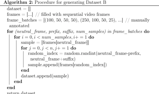
Next, we select a group of frames that contain the subject character in a neutral pose. We also identify a range of nearby frames that depict the character in non-neutral poses and a number 𝑛 of samples to construct. To construct Dataset B from a sequential list of video frames, we execute Algorithm 2. After running this procedure, we can generate datasets like Dataset B, for example, which feature human subjects and allow us to capture and attempt to reproduce realistic human-like deformations. Example samples from Dataset B are shown in Figure 3-5.

3.3

Network Structure

Given our input specification, we present a specific neural network architecture for use with Dataset A and Dataset B (and similar datasets) as shown in Figure 3-6.

Algorithm 2: Procedure for generating Dataset B dataset = []

frames = [...] // filled with sequential video frames

frame_batches = [(100, 50, 50, 50), (250, 100, 50, 25), ...] // manually annotated

for (neutral_frame, prefix, suffix, num_samples) in frame_batches do for 𝑖 = 0, 𝑖 < 𝑛𝑢𝑚_𝑠𝑎𝑚𝑝𝑙𝑒𝑠, 𝑖+ = 1 do sample = [frames[neutral_frame]] for 𝑗 = 0, 𝑗 < 𝑛, 𝑗+ = 1 do random_index = random.randint(neutral_frame-prefix, neutral_frame+suffix) sample.append(frames[random_index]) end dataset.append(sample) end end return dataset

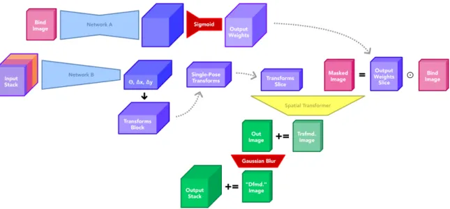
During training, we first generate a block of attachment weights as shown in the top of Figure 3-6 with Network A. Next, we generate affine transformation matrices with Network B. We deform the input bind image 𝑛 times with these transformation matrices and attachment weights to generate 𝑛 output images. Finally, we augment our output tensor with a modified attachment weights block to strengthen our results.

Figure 3-5: Two samples from Dataset B featuring realistic characters with 𝑛 = 4 target images (images sampled from [1])

Figure 3-6: Specific network architecture for deforming images

3.3.1

Weights Generation

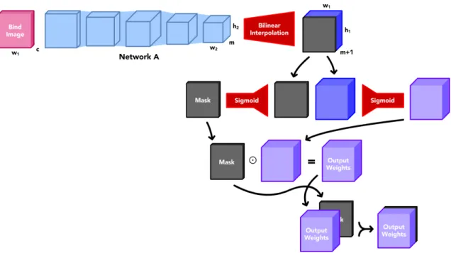
Figure 3-7: Network A and auxiliary structures

The precise structure of Network A is shown in Figure 3-7. This network uti-lizes convolution, max pooling, and resizing layers to generate a block of attachment weights from a bind image. Attachment weights for use in animation should, at minimum, adhere to the following constraints:

∙ All weights should sum to 1.0 for each vertex over all skeleton joints (referred to as partition of unity)

∙ For each joint, the distribution of weights should be 𝐶1 continuous

Therefore, to enforce partition of unity, we apply the sigmoid function to the generated attachment weights block across all skeleton joints. Though we cannot

guarantee 𝐶1 continuity with this approach, we assume that any generated

distribu-tion of weights for any joint can be approximated with a 𝐶1 continuous distribution

sufficiently enough for our purposes.

3.3.2

Masking

This specific architecture can be slightly modified to support bind images with back-grounds. Network A and its auxiliary structures can be augmented as shown in Figure 3-8 to mask bind images.

Figure 3-8: Network A and auxiliary structures w/ masking support

Note that the sigmoid function is not applied to generated masks as part of the attachment weights block. Rather, the sigmoid function is applied to masks indepen-dently to limit their single-channel range to between 0.0 and 1.0. Though optional, masking may prove useful for artists who would prefer to use images of characters with unmasked backgrounds as inputs to this system.

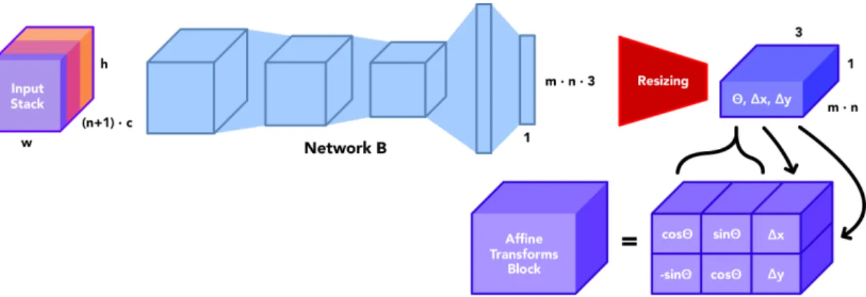
Figure 3-9: Network B and auxiliary structures

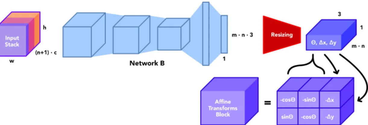
3.3.3

Transform Generation

The precise structure of Network B is shown in Figure 3-9. This network utilizes primarily convolution and max pooling layers to process the entire input stack (in-cluding all target images) and generate a small block of values representing 𝜃, ∆𝑥 and ∆𝑦 for all 𝑛 target images and 𝑚 joints. Every 𝜃, ∆𝑥 and ∆𝑦 is used to construct a block of affine transformation matrices as shown in Figure 3-9 by using differentiable trigonometric functions.

3.3.4

Differential Rendering

After producing attachment weights and affine transformations with Network A and Network B, we employ spatial transformer networks to deform each bind image with LBS as shown in Equation 3.1: 𝑣′_𝑖 = ( 𝑚 ∑︁ 𝑗=1 𝑇𝑗𝑤𝑖𝑗)𝑣𝑖 (3.1)

Here, 𝑣𝑖 refers to the position of the 𝑖𝑡ℎvertex in the character mesh, 𝑇𝑗 represents

the affine transformation corresponding to joint 𝑗, and 𝑤𝑖𝑗 represents the weight

linking vertex 𝑣𝑖 to joint 𝑗. The attachment weights we learn from Network A can be

substituted in for 𝑤𝑖𝑗, and the affine transformations we learn from Network B can

be substituted in for 𝑇𝑗. To compute 𝑣

′

𝑖, we feed this data with our bind image into

Spatial transformer networks can be implemented with some machine learning frameworks by organizing data into a grid, transforming the grid with some affine transformation, and sampling the resulting grid to produce an output tensor. In practice, each iteration of this procedure can significantly impact runtime. Imple-menting Equation 3.1 requires us to run this procedure for every vertex 𝑣𝑖 of the bind

image in each training sample, which incurs a significant runtime penalty. Therefore, we instead use an approximation of LBS that mitigates these performance issues, as shown in Equation 3.2: 𝐵[𝑣𝑖] = 𝑚 ∑︁ 𝑗=1 𝐴[𝑇_𝑗−1𝑣𝑖] · 𝑤𝑖𝑗 (3.2)

Here, 𝑣𝑖 refers to the position of the 𝑖𝑡ℎ vertex in the character mesh, 𝐵 refers

to the output mesh, 𝐴 refers to the bind image or input mesh, 𝑇_𝑗−1 represents the inverse of the affine transformation for joint 𝑗, and 𝑤𝑖𝑗 represents the weight linking

vertex 𝑣𝑖 to joint 𝑗. With this formulation, we calculate 𝐴[𝑇𝑗−1𝑣𝑖] · 𝑤𝑖𝑗 once per joint 𝑗

by utilizing hardware optimizations to element-wise multiply 𝐴 by a weight channel 𝑤𝑗. Therefore, because we only need to use spatial transformer networks to compute

𝐴[𝑇_𝑗−1𝑣𝑖] for 𝑚 times, we can significantly reduce the runtime penalty incurred by

using the formulation from Equation 3.1. This formulation also slightly modifies our affine transformation generation pipeline, which we alter to generate inverse affine transforms 𝑇_𝑗−1 as shown in Figure 3-10.

Figure 3-10: Network B and auxiliary structures, generates inverse affine transforma-tions

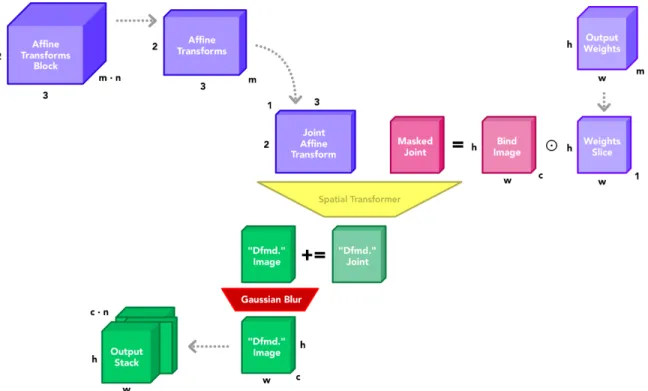
Figure 3-11: Differential rendering pipeline and auxiliary structures for use during training

We use this formulation to transform masked copies of the bind image 𝑚 · 𝑛 times and construct an output stack as shown in Figure 3-11. First, the bind image is copied 𝑚 times (𝑚 represents the number of desired joints in the character and the number of unique channels in our attachment weights block). Next, each copy of the bind image is multiplied by the corresponding channel of weights from the generated attachment weights block. Effectively, each channel of weights acts as a mask on the bind image that is tuned during training to isolate a single rigid component of the bind-posed character. We also extract the appropriate affine transformation grid for the current joint of the current target pose. Next, we use a spatial transformer network to transform each of these masked images according to Equation 3.2. We stack these transformed components together into a single output image corresponding to the current target pose. Lastly, we stack 𝑛 of these images together into one output stack. This output stack is returned and compared against a reference stack to calculate loss and begin backpropagation through both Network A and Network B.

3.3.5

Regularization

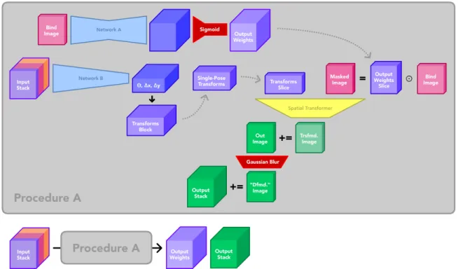
To strengthen our training objective and make our results more robust, we augment our output stack with data generated during training. Most of the system that we have discussed thus far can be grouped into a single procedure as shown in Figure 3-12. Note that we can extract both an output stack of deformed images and a block of attachment weights as outputs from one iteration of Procedure A.

Figure 3-12: Procedure abstraction of entire system

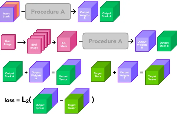
During one iteration of training, we run Procedure A once to generate an output stack (denoted Stack A) and a block of attachment weights (denoted Weights A). Next, we run Procedure A again with an alternate input stack to generate another output stack (denoted Stack B) and another block of attachment weights (denoted Weights B). The alternate input stack that we use is constructed by copying the original bind image 𝑛 + 1 times and stacking them images together. This alternate input stack represents a dataset sample with the original neutral image and 𝑛 target neutral-pose images to reproduce. We then augment Stack A and its reference stack by concatenating Weights A and Weights B respectively. By comparing these new

output tensors to calculate loss for backpropagation, we reinforce Network A’s ability to generate consistent weights. This entire process is shown in detail in Figure 3-13.

Figure 3-13: Utilization of Procedure A during one iteration of training

3.4

Training Methodology

This entire system can be tuned with a small collection of hyperparameters, in-cluding the learning rate and batch size. For our testing, we used the Adam optimizer [11], an initial learning rate around 2.2 × 10−4, a batch size of 8, and trained the en-tire system for between 500 to 1000 epochs to achieve the best empirical results. We use the 𝐿2 loss function as shown in Equation 3.3 to begin backpropagation during

training. In Equation 3.3, 𝑥 represents an input sample (i.e., the Input Stack shown in Figure 3-13), 𝑦𝑖 represents a reference output sample (i.e., the Target Tensor shown

in Figure 3-13), and 𝑦_𝑖* represents a generated output sample (i.e., the Output Ten-sor shown in Figure 3-13). We also limit the number of samples within our testing

datasets to around 500 because of performance limitations, which implies that our trained networks may be significantly overfit. We expect trained networks to be over-fit with small single-character datasets like Dataset A and Dataset B, though ideally this system would be trained with large multi-character datasets to accommodate for a wide range of inputs at run time. Larger datasets can be easily constructed, and we speculate that training with a sufficiently large and diverse dataset will mitigate overfitting issues.

3.4.1

Alternative Training Methods

Many other parameters of our system can also be tuned to achieve different results. One such parameter is the size of the weights block produced from Network A as shown in Figure 3-7. 𝑤2 and ℎ2 are typically smaller than 𝑤1 and ℎ1 respectively

with most system configurations. 𝑤2 and ℎ2 are determined by the number of

con-volutional layers, number of max pooling layers, and padding techniques used inside Network A. Typically, a single convolutional layer will reduce the size of its input tensor when padding is not used, which is demonstrated in Figure 3-14. Therefore, more convolutional layers in Network A typically implies a smaller generated weights texture size. These generated weights are resized using bilinear interpolation to match the dimensions of the input bind image. There is an apparent tradeoff from changing the values for 𝑤2 and ℎ2: when 𝑤2 and ℎ2 are small, Network A may converge faster

to produce weights capable of isolating character components during training, albeit with smoother boundaries. When 𝑤2 and ℎ2 are large, however, Network A may

produce weights with harsher boundaries between channels and delineate component boundaries more explicitly. In our testing, the system produces the best results with 𝑤2 and ℎ2 set to about 75% of the values of 𝑤1 and ℎ1 respectively.

Another parameter worth exploring is 𝑚, the number of desired joints to extract from a character. When 𝑚 is small (i.e., set to around 2-5 joints), the system may struggle to accurately recreate target images while training, regardless of generated transforms. For instance, after training the system with Dataset A and using 𝑚 = 5, many weight channels converged to include a large portion of the character or failed to

Figure 3-14: Convolution without pooling around edges

converge altogether. When 𝑚 is large, however, many weight channels may converge to isolate negligible parts of the input character, like a small part of the character’s foot. Therefore, to generate appropriately useful and realistic attachment weights, it is best to set 𝑚 qualitatively such that 𝑚 disconnected limbs on a character could be found and transformed to reasonably approximate any realistic pose. We discuss this phenomenon further in section 5.1.1. For Dataset A, we set 𝑚 = 13 to approximate the actual 15 joints used to generate each character in Dataset A.

In addition, the method for producing affine transformations as depicted in Figure 3-10 can also be modified. Instead of generating 𝜃, ∆𝑥 and ∆𝑦 and constructing an affine transformations block with trigonometric functions, you can consider learning the affine transformations block directly as an output of Network B. Again, however, there are tradeoffs to this method: By directly learning the affine transformations block, transformations can include skewing and resizing as well as rotation and trans-lation. This may be inappropriate for modeling characters that typically move rigidly, like those featured in Dataset A. This may be appropriate, though, for modeling more elastic characters, like exaggerated cartoons.

3.4.2

Staggered Training

Temporarily locking some networks during training can also yield different results. For instance, Network B may be locked for some ℎ number of epochs while Network A is being tuned during training. Training procedures like this may be useful when using datasets with low pose variance between bind images and target images. The affine transformations block is configured with random values prior to training, so locking Network B while training Network A may force the system to utilize static, non-uniform transforms and help the system converge to a solution more capable of isolating character components.

Situations may arise where a network (or part of a network) may quickly collapse to produce identical outputs. For example, when the masking procedure shown in Figure 3-8 is implemented, Network B quickly and consistently converges after 2 to 5 epochs of training to produce attachment weights that equal 1.0 across one entire channel and equal 0.0 everywhere else. This results in output images that all resemble their corresponding input bind images that have been rotated and slightly translated (as shown in Figure 3-15), which are hardly desireable results. To avoid this issue, we lock the mask-generation portion of Network B for the first 10 to 20 epochs of training. After training concludes, output images appropriately resemble their corresponding target images. All technical results are discussed further in Chapter 4.

Chapter 4

Results

After one iteration of Procedure A (as depicted in Figure 3-12), we can extract a block of attachment weights and a stack of output images. After each epoch of training, we run Procedure A with a randomly-selected dataset sample and render the generated images and weights to disk. Once training concludes, we can study these saved images and weights to assess the system’s performance as training progresses.

4.1

Output Images

We trained our architecture on a subset of Dataset A for 500 epochs. We show the generated output images at intermediate stages in Figure 4-1. For this training ses-sion, we set 𝑛 = 4, which is reflected in the 𝑛 number of target images and output images produced at each epoch. We can verify our LBS approximation (Equation 3.2) by examining the images for Epoch 1 in Figure 4-1; the bind image is copied 𝑚 = 13 times, each copy is masked by a channel of weights, and stacked together into one output image. We can also verify that our system becomes more capable of reproducing the target images as training progresses. After 500 epochs of training, the system has been tuned to produce output images that closely resemble the cor-responding target images, though some artifacts remain visible, like faint shadows of different character components present where clear space exists in the corresponding target images.

Figure 4-1: Intermediate output images with one sample from Dataset A

Figure 4-2: Loss per epoch during training session with Dataset A (blue line marks training set loss, orange line marks testing set loss)

An analysis of the loss plot (as shown in Figure 4-2) for this training session reveals that loss had begun stabilizing (ignoring perturbations) before epoch 500 of training, which implies that the system’s networks had been tuned sufficiently to reach a locally-optimal solution. The perturbations in the loss plot also imply that a smaller learning rate may be necessary to achieve marginally better results. The divergence between the training set loss (shown in blue) and the testing set loss (shown in orange) also suggests that the system is significantly overfitting to the subset of Dataset A we use for training.

Figure 4-3: Intermediate output images with one sample from Dataset B

We also trained our architecture on a subset of Dataset B for 800 epochs. We show the generated output images for this session at intermediate stages in Figure 4-3. We use similar hyperparameters and set 𝑛 = 4 and 𝑚 = 10. Again, as training concludes, the output images show a close resemblance with their corresponding target images despite also featuring similar artifacts.

Figure 4-4: Loss per epoch during training session with Dataset B (blue line marks training set loss, orange line marks testing set loss)

An analysis of the loss plot (as shown in Figure 4-4) for this training session reveals that loss had not quite finished stabilizing (ignoring perturbations) before epoch 800 of training. Similar to our training session with Dataset A, the divergence between the training set loss (shown in blue) and the testing set loss (shown in orange) suggests that the system is significantly overfitting to the subset of Dataset B we use for training.

4.2

Output Attachment Weights

For our training session with Dataset A, we set the number of desired joints 𝑚 to 13. Therefore, the generated output weights contain 13 channels. In Figure 4-5, we show a block of generated weights using a randomly-selected input sample after one epoch of training. These weights show a near-uniform distribution of weights across all 𝑚 bones. At this stage of training, weights channels do not appear to be isolating different components of the character. In Figure 4-6, we show a block of generated weights using a randomly-selected input sample after 500 epochs of training. These

Figure 4-5: Output attachment weights after 1 epoch of training with Dataset A, exposure increased to highlight weight channels

weights show clear emphasis on different components of the character from channel to channel. Many weight channels show a distinct boundary between neighboring components, implying the existence and recognition of a rigid connection between components in that region.

We produce a similar set of weights from our training session with Dataset B with 𝑚 = 10. In Figure 4-7, we show a block of generated weights using a randomly-selected input sample after 800 epochs of training. Again, these weights show clear emphasis on different character components similarly to the weights shown in Figure 4-6, implying that this approach can produce similar results with non-synthetic data.

Figure 4-6: Output attachment weights after 500 epochs of training with Dataset A

4.3

Evaluating Attachment Weights

To evaluate the efficacy of generated weights, we develop our own custom animation tool to produce deformed images of an input bind image using LBS (Equation 3.1). This animation tool, like many other professional animation tools, requires a skeleton (comprised of hierarchically-linked joints) to be defined for an input character model. We can translate and rotate these joints to deform the character model into new poses.

Figure 4-8: Procedure outline for rigging characters with generated attachment weights

Figure 4-8 outlines a typical procedure for rigging characters with generated weights. The first character shows the shape of the character model. The second character shows the distribution of generated attachment weights across the model (each color indicates a unique channel of weights). The third character illustrates where to choose control points or joints to manipulate for animation. The last char-acter highlights the definition of a hierarchical skeleton using the established joints. This skeleton propagates transformations from parent joints down to child joints such that, for example, rotating a shoulder joint realistically affects the position and rota-tion of an elbow or wrist joint. For more informarota-tion on this process, which is known as forward kinematics, refer to [15].

There exist many ways to choose joint positions given a block of attachment weights. In our custom animation pipeline, we choose joint positions by calculating the average weighted position through a weight channel as shown in Algorithm 3. We

can also choose joint positions by finding the position of the maximum-weight element in each weight channel, manually annotating positions, or by using some alternate method.

Algorithm 3: Example procedure for selecting joint positions

weights = [...] // automatically generated, has shape (width, height, channels)

joint_positions = []

for 𝑖 = 0, 𝑖 < 𝑤𝑒𝑖𝑔ℎ𝑡𝑠.𝑠ℎ𝑎𝑝𝑒[2], 𝑖+ = 1 do weight_channel = weights[:, :, i]

indices_grid = np.indices(weight_channel.shape) weighted_positions = weight_channel * indices_grid pos_x = np.sum(weighted_positions[:, :, 0])

pos_y = np.sum(weighted_positions[:, :, 1]) joint_positions.append((pos_x, pos_y)) end

return joint_positions

Figure 4-9: Example deformation using custom animation pipeline and idealized weights

Using our custom animation pipeline, we are able to deform input characters from Dataset A with idealized weights as shown in Figure 4-9. In comparison, we use the same pipeline to deform input characters from Dataset A with generated weights as shown in Figure 4-10. Deformations using generated weights appear to "stretch" more near component boundaries, which occurs because of soft component boundaries in the generated weights themselves. Additional deformation results from our training sessions with Dataset A are shown in Figure 4-11, and deformation results from our

Figure 4-10: Example deformation using custom animation pipeline and generated weights

training sessions with Dataset B are shown in Figure 4-12.

Interestingly, most characters (both synthetic and non-synthetic) can be some-what realistically deformed with small joint transformations, which demonstrates the effectiveness of this entire approach for generating attachment weights. Additional output weights, deformation figures, and dissected animations are included in Ap-pendix A.

Figure 4-11: Example deformations from Dataset A using custom animation pipeline and generated weights

Figure 4-12: Example deformations from Dataset B using custom animation pipeline and generated weights

Chapter 5

Conclusion

5.1

Limitations

Despite the promise of this approach, it has many limitations. Neural networks in general are still not well understood, and more research and exploration is needed to identify causes and solutions for neural network-related issues, like diminishing gradients [20] and mode collapse [19]. In addition to these issues, we also identify several issues specific to our architecture and discuss potential solutions and mitiga-tion strategies.

5.1.1

Disconnected Components

During many training sessions with this system, multiple character components are grouped together in a single channel from the attachment weights generated from Network B (as seen in Figure 3-10). Frequently, these grouped components are dis-connected in the character model itself, like the example shown in Figure 5-1. In an animation workflow, this implies that both components will be linked to the same joint and will share the same transformation, which is typically unrealistic and undesirable behavior.

This issue may be caused by setting 𝑚, the number of desired joints and weight channels, too low. As mentioned in section 3.4.1, choosing 𝑚 is a qualitative task

Figure 5-1: Aggressive component grouping problem example

informed by the complexity of the character(s) you wish to deform – the correct value for 𝑚 must not be too low nor too high, but these exact bounds are difficult to ascertain precisely. If we assume some dataset, like Dataset A, was constructed with characters using some exact 𝑚* number of joints, then at least 𝑚* joints (and weight channels) will be needed by our system to accurately recreate the character’s original skeleton and components. Any number of joints less than 𝑚* will force some weight channels to, in the best case scenario, group multiple character components together, resulting in the issue shown in Figure 5-1. Therefore, there exists some lower bound 𝑚* inherent in every dataset, and 𝑚 must be greater than or equal to 𝑚* for our system to produce accurate results. For non-synthetic datasets, like Dataset B, 𝑚* is unknown, meaning 𝑚 must be chosen qualitatively as depicted in Figure 5-2.

Even if 𝑚* is known and we choose some 𝑚 ≥ 𝑚*, there is no guarantee that all 𝑚 weight channels will be used to isolate character components. We can encour-age at least 𝑚* weight channels to be used, however, by constructing datasets with enough images to demonstrate non-coupled behavior between all pairs of character components. This forces the system to learn to transform each character component independently in order to replicate the poses from each training sample.

There can be other causes for this issue, however. Idiosyncrasies and unintentional gaps in datasets may also cause aggressive grouping issues in generated weights. In fact, many seemingly-negligible properties of datasets can significantly alter the ac-curacy of this system, which we discuss further in section 5.1.2.

Figure 5-2: Qualitative procedure for determining 𝑚 for a non-synthetic character

5.1.2

Dataset Sensitivity

As mentioned earlier, many dataset properties can drastically alter the effectiveness of this system. One such property is pose variance, or rather the image-to-image variance between character component transformations. When pose variance is low (i.e., all characters in a given dataset have very similar poses), Network A may become tuned to produce weight channels that aggressively group multiple character components together. When pose variance is too high, however, the entire system may struggle to converge to a reasonable solution. Therefore, dataset samples must demonstrate some appropriately moderate amount of variance between poses for the system to produce desireable results. For example, Figure 5-3 shows results from two different training sessions using different datasets. The left-hand session used a variant of Dataset A with low pose variance – for instance, each target image shows thigh and shin components transforming closely together as if rigidly coupled. The right-hand session used a variant of Dataset A with moderate pose variance – each target image demonstrates more independent behavior between character components. As a result, the left-hand session produced output weights with aggressive component grouping (indicated by repetition of colors in the colorized weights diagram) whereas the right-hand session produced weights where component grouping is less aggressive.

Figure 5-3: Effects of pose variance on system outputs

5.2

Future Extensions

Regardless of these issues, this approach remains promising primarily due to its exten-sibility and versatility. By simply constructing a new dataset following the guidelines discussed in section 3.2, this approach can be easily adapted for new domains. There are some additional extensions, however, that could expand the capabilities of this approach even further.

Currently, this system is limited to process and produce 2D images and accompa-nying weights, but by modifying the system’s network structures and differentiable rendering pipeline, 3D models and weights could be supported. Then, a system like this could be utilized for 3D visual effects and 3D animated films.

This approach also currently approximates LBS (Equation 3.1) to deform bind images inside a differentiable rendering pipeline. A different deformation technique could be substituted in for LBS, like Dual Quaternion Skinning [10], which may yield more accurate results. Such a deformation technique may need to be approximated (similarly to how Equation 3.2 approximates Equation 3.1) to improve training per-formance, but a close approximation may still yield accurate results.

Figure 5-4: Potential extension of sample format

Also, if we consider alternate use cases, we can extend this system by including more data in each dataset sample. We designed this system to enable artists to produce effective attachment weights for a character by running Network A with a single image of this character as input. Additional information may be helpful while generating attachment weights, however, and may not be difficult for artists to provide. Joint position estimates, for example, could be incorporated into each input sample as shown in Figure 5-4 and used to inform Network A to construct more desireable attachment weights. At runtime, artists could place joint markers onto a character image, which could be interpreted and used as inputs to Network A for generating attachment weights.

Appendix A

Additional Results

Figure A-1: Example deformations for input sample from Dataset A using custom animation pipeline and generated weights

Figure A-2: Example deformations for input sample from Dataset A using custom animation pipeline and generated weights

Figure A-3: Additional example deformations from Dataset A using custom animation pipeline and generated weights

Figure A-4: Dissected animation using generated weights and sample from Dataset A, masking enabled

Figure A-5: Dissected animation using generated weights and sample from Dataset B

Bibliography

[1] Dancing in front of the Green Screen. Feb 2017. [2] Maya - Joints and IK Handles. Sep 2017.

[3] Rigging for Beginners: Painting Weights in Maya. Dec 2019. [4] Autodesk, INC. Maya.

[5] Stephen W. Bailey, Dave Otte, Paul Dilorenzo, and James F. O’Brien. Fast and deep deformation approximations. ACM Transactions on Graphics, 37(4):119:1– 12, August 2018. Presented at SIGGRAPH 2018, Los Angeles.

[6] Ilya Baran and Jovan Popović. Automatic rigging and animation of 3d characters. ACM Transactions on graphics (TOG), 26(3):72–es, 2007.

[7] Andrew Feng, Dan Casas, and Ari Shapiro. Avatar reshaping and automatic rigging using a deformable model. In Proceedings of the 8th ACM SIGGRAPH Conference on Motion in Games, pages 57–64, 2015.

[8] Lisa Fridsma and Brie Gyncild. Adobe After Effects CC Classroom in a Book (2017 Release). Adobe Press, 1st edition, 2017.

[9] Alec Jacobson, Ilya Baran, Jovan Popović, and Olga Sorkine. Bounded bihar-monic weights for real-time deformation. ACM Transactions on Graphics (pro-ceedings of ACM SIGGRAPH), 30(4):78:1–78:8, 2011.

[10] Alec Jacobson, Zhigang Deng, Ladislav Kavan, and JP Lewis. Skinning: Real-time shape deformation. In ACM SIGGRAPH 2014 Courses, 2014.

[11] Diederik P. Kingma and Jimmy Ba. Adam: A method for stochastic optimiza-tion, 2014.

[12] Binh Huy Le and Zhigang Deng. Robust and accurate skeletal rigging from mesh sequences. ACM Transactions on Graphics (TOG), 33(4):1–10, 2014.

[13] John P Lewis, Matt Cordner, and Nickson Fong. Pose space deformation: a unified approach to shape interpolation and skeleton-driven deformation. In Proceedings of the 27th annual conference on Computer graphics and interactive techniques, pages 165–172, 2000.

[14] Lijuan Liu, Youyi Zheng, Di Tang, Yi Yuan, Changjie Fan, and Kun Zhou. Neu-roskinning: Automatic skin binding for production characters with deep graph networks. ACM Transactions on Graphics (TOG), 38(4):1–12, 2019.

[15] Richard M. Murray, S. Shankar Sastry, and Li Zexiang. A Mathematical Intro-duction to Robotic Manipulation. CRC Press, Inc., USA, 1st edition, 1994. [16] Omid Poursaeed, Vladimir G. Kim, Eli Shechtman, Jun Saito, and Serge

Be-longie. Neural puppet: Generative layered cartoon characters, 2019.

[17] Mahdi Rad and Vincent Lepetit. Bb8: A scalable, accurate, robust to partial occlusion method for predicting the 3d poses of challenging objects without using depth. In Proceedings of the IEEE International Conference on Computer Vision, pages 3828–3836, 2017.

[18] Yurui Ren, Xiaoming Yu, Junming Chen, Thomas H. Li, and Ge Li. Deep image spatial transformation for person image generation, 2020.

[19] Hoang Thanh-Tung and Truyen Tran. On catastrophic forgetting and mode collapse in generative adversarial networks, 2018.

[20] Joost van Doorn. Analysis of deep convolutional neural network architectures. 2014.