EUROPEAN ORGANISATION FOR NUCLEAR RESEARCH (CERN)
Eur. Phys. J. C 79 (2019) 836
DOI:DOI:10.1140/epjc/s10052-019-7335-x
CERN-EP-2019-085 18th November 2019
Identification of boosted Higgs bosons decaying into
b-quark pairs with the ATLAS detector at 13 TeV
The ATLAS Collaboration
This paper describes a study of techniques for identifying Higgs bosons at high transverse momenta decaying into bottom-quark pairs, H → b ¯b, for proton–proton collision data collected by the ATLAS detector at the Large Hadron Collider at a centre-of-mass energy
√
s = 13 TeV. These decays are reconstructed from calorimeter jets found with the anti-kt R = 1.0 jet
algorithm. To tag Higgs bosons, a combination of requirements is used: b-tagging of R = 0.2 track-jets matched to the large-R calorimeter jet, and requirements on the jet mass and other jet substructure variables. The Higgs boson tagging efficiency and corresponding multijet and hadronic top-quark background rejections are evaluated using Monte Carlo simulation. Several benchmark tagging selections are defined for different signal efficiency targets. The modelling of the relevant input distributions used to tag Higgs bosons is studied in 36 fb−1of data collected in 2015 and 2016 using g → b ¯b and Z(→ b ¯b)γ event selections in data. Both processes are found to be well modelled within the statistical and systematic uncertainties.
© 2019 CERN for the benefit of the ATLAS Collaboration.
Reproduction of this article or parts of it is allowed as specified in the CC-BY-4.0 license.
1 Introduction
The Large Hadron Collider (LHC) centre-of-mass energy of 13 TeV greatly extends the sensitivity of the ATLAS experiment [1] to heavy new particles. In several new physics scenarios [2–4], these heavy new particles may have decay chains including the Higgs boson [5,6]. The large mass-splitting between these resonances and their decay products results in a high-momentum Higgs boson, causing its decay products to be collimated. The decay of the Higgs boson into a b ¯b pair has the largest branching fraction within the Standard Model (SM), and thus is a major decay mode to use when searching for resonances involving high-momentum Higgs bosons (see e.g. Ref. [7]), as well as for measuring the SM Higgs boson properties. The signature of a boosted Higgs boson decaying into a b ¯b pair is a collimated flow of particles, in this document called a ‘Higgs-jet’, having an energy and angular distribution of the jet constituents consistent with a two-body decay and containing two b-hadrons. The techniques described in this paper to identify Higgs bosons decaying into bottom-quark pairs have been used successfully in several analyses [8–10] of 13 TeV proton–proton collision data recorded by ATLAS.
In order to identify, or tag, boosted Higgs bosons it is paramount to understand the details of b-hadron identification and the internal structure of jets, or jet substructure, in such an environment [11]. The approach to tagging presented in this paper is built on studies from LHC runs at
√
s = 7 and 8 TeV, including extensive studies of jet reconstruction and grooming algorithms [12], detailed investigations of track-jet-based b-tagging in boosted topologies [13], and the combination of substructure and b-tagging techniques applied in the Higgs boson pair search in the four-b-quark final state [14] and for discrimination of Z bosons from W bosons [15]. Gluon splitting into b-quark pairs at small opening angles has been studied at
√
s = 13 TeV by ATLAS [16]. The identification of Higgs bosons at high transverse momenta through the use of jet substructure has also been studied by the CMS Collaboration and their techniques are described in Refs. [17,18].
The Higgs boson tagging efficiency and background rejection for the two most common background processes, the multijet and hadronic top-quark backgrounds, are evaluated using Monte Carlo simulation. In addition, two processes with a topology similar to the signal, Z → b ¯b decays and g → b ¯b splitting, are used to validate Higgs-jet tagging techniques in data at
√
s = 13 TeV. In particular the modelling of relevant Higgs-jet properties in Monte Carlo simulation is compared with data. The g → b ¯b process allows the modelling of one of the main backgrounds to be validated. The Z → b ¯b process is a colour-singlet resonance with a mass close to the Higgs boson mass and thus very similar to the H → b ¯b signal. After a brief description of the ATLAS detector in Section2and of the data and simulated samples in Section3, the object reconstruction, selection and labelling is discussed in Section4. Section5describes relevant systematic uncertainties. The Higgs-jet tagging algorithm and its performance are presented in Section6. Sections7and8discuss a comparison between relevant distributions in data control samples dominated by g → b ¯b and Z(→ b ¯b)γ and the corresponding simulated events, respectively. Finally, conclusions are presented in Section9.
2 ATLAS detector
The ATLAS detector [1] at the LHC covers nearly the entire solid angle around the collision point.1 It consists of an inner tracking detector surrounded by a thin superconducting solenoid, electromagnetic and hadronic calorimeters, and a muon spectrometer incorporating three large superconducting toroid magnets. The inner-detector system (ID) is immersed in a 2 T axial magnetic field and provides charged-particle tracking in the range |η| < 2.5.
Preceding data-taking at a centre-of-mass energy of 13 TeV, the high-granularity silicon pixel detector was equipped with a new barrel layer, located at a smaller radius (of about 34 mm) than the other layers [19,20]. The upgraded pixel detector covers the vertex region and typically provides four measurements for tracks originating from the luminous region. It is followed by a silicon microstrip tracker, which usually provides four space points per track. These silicon detectors are complemented by a transition radiation tracker, which enables radially extended track reconstruction up to |η| = 2.0. The transition radiation tracker also provides electron identification information based on the fraction of hits above a certain energy deposit threshold corresponding to transition radiation.
The calorimeter system covers the pseudorapidity range |η| < 4.9. Within the region |η| < 3.2, electromagnetic calorimetry is provided by barrel and endcap high-granularity lead/liquid-argon (LAr) calorimeters, with an additional thin LAr presampler covering |η| < 1.8 to correct for energy loss in material upstream of the calorimeters. Hadronic calorimeter within |η| < 1.7 is provided by a steel/scintillating-tile calorimeter, segmented into three barrel structures, and two copper/LAr hadronic endcap calorimeters covering 1.5 < |η| < 3.2. The solid angle coverage is completed with forward copper/LAr and tungsten/LAr calorimeter modules optimised for electromagnetic and hadronic measurements respectively.
The muon spectrometer (MS) comprises separate triggering and high-precision tracking chambers measuring the deflection of muons in a magnetic field generated by superconducting air-core toroids. The precision chamber system covers the region |η| < 2.7 with three layers of monitored drift tubes, complemented by cathode strip chambers in the forward region, where the background is highest. The muon trigger system covers the range |η| < 2.4 with resistive plate chambers in the barrel, and thin gap chambers in the endcap regions.
A two-level trigger system is used to select interesting events [21]. The level-1 trigger is implemented in hardware and uses a subset of detector information to reduce the event rate to a design value of at most 100 kHz. This is followed by a software-based high-level trigger, which reduces the event rate further to an average of 1 kHz.
3 Data and simulated event samples
The data used in this paper were recorded with the ATLAS detector during the 2015 and 2016 LHC proton– proton (pp) collision runs, and correspond to a total integrated luminosity of 36.1 fb−1at
√
s = 13 TeV. This integrated luminosity is calculated after the imposition of data quality requirements, which ensure that the ATLAS detector was in good operating condition.
1 ATLAS uses a right-handed coordinate system with its origin at the nominal interaction point (IP) in the centre of the detector
and the z-axis along the beam pipe. The x-axis points from the IP to the centre of the LHC ring, and the y-axis points upwards. Cylindrical coordinates (r, φ) are used in the transverse plane, φ being the azimuthal angle around the z-axis. The pseudorapidity is defined in terms of the polar angle θ as η = − ln tan(θ/2). Angular distance is measured in units of ∆R ≡
p
Several Monte Carlo (MC) simulated event samples were used for the optimisation of the Higgs boson tagger, estimation of its performance, and the comparisons between data and simulation.
Simulated events with a broad transverse momentum (pT) spectrum of Higgs bosons were generated as
decay products of Randall–Sundrum gravitons G∗in a benchmark model with a warped extra dimension [2], G∗ → HH → b ¯bb ¯b, over a range of graviton masses between 300 and 6000 GeV. The events were simulated using the MadGraph5_aMC@NLO generator [22]. Parton showering, hadronisation and the underlying event were simulated with Pythia8 [23] using the leading-order (LO) NNPDF2.3 parton distribution function (PDF) set [24] and the ATLAS A14 [25] set of tuned parameters.
Events containing the Z (→ b ¯b)γ and γ + jets processes were simulated with the Sherpa v2.1.1 [26–29] LO generator. The matrix elements were configured to allow up to three partons in the final state in addition to the Z boson or the photon. The Z boson was produced on-shell and required to decay hadronically. The CT10 next-to-leading-order (NLO) PDF set [30,31] was used. The t ¯tγ MC events were modelled by MadGraph interfaced with Pythia8 for showering, hadronisation and the underlying event with the LO NNPDF2.3 PDF set and the A14 underlying-event tune. Simulated events of hadronically decaying W γ were generated using Sherpa v2.1.1, with the same configuration as the one used for the Z γ sample. To cover a large range of top-quark transverse momenta, hadronically decaying top quarks were generated using Z0bosons decaying into t ¯t pairs over a range of Z0boson masses between 400 and 5000 GeV. These samples were simulated using Pythia8 with the LO NNPDF2.3 PDF set and the A14 underlying-event tune.
Finally, inclusive multijet events were generated using Pythia8, with the LO NNPDF2.3 PDF set and the A14 underlying-event tune; and with Herwig++ [32], with the CTEQ [33] PDF set and the UEEE [34] underlying event tune. To increase the number of simulated events with semimuonically decaying hadrons for the g → b ¯b analysis, samples of multijet events filtered to have at least one muon with pTabove 3 GeV
and |η| < 2.8 were produced with Pythia8 and Herwig++ using the same PDF set and underlying-event tunes as the unfiltered multijet samples.
In all cases except events generated using Sherpa, EvtGen [35] was used to model the decays of b- and c-hadrons. All simulated event samples included the effect of multiple pp interactions in the same and neighbouring bunch crossings (‘pile-up’) by overlaying simulated minimum-bias events on each simulated hard-scatter event. The minimum-bias events were simulated with the single-, double- and non-diffractive pp processes of Pythia8 using the A2 tune [36] and the MSTW2008 LO PDF [37–39]. The detector response to the generated events was simulated with Geant 4 [40,41].
4 Object and event reconstruction
In this section the object reconstruction, associations among the objects, jet labelling, and the procedure to determine the heavy-flavour content of jets are described.
Calorimeter jets: Calorimeter-based jets are built from noise-suppressed topological clusters and are
reconstructed using FastJet [42] with the anti-kt algorithm [43] with a radius parameter of R = 1.0 (large-R jets) or R = 0.4 (small-R jets). The topological clusters of the large-R jets are brought to the hadronic energy scale using the local hadronic cell weighting scheme [44]. The large-R jets are groomed using trimming [12,45] to discard the softer components of jets that originate from initial-state radiation, pile-up interactions or the underlying event. This is done by reclustering the constituents of the initial jet,
using the kt algorithm [46,47], into subjets of radius parameter Rsub= 0.2 and removing any subjet that
has a pTless than 5% of the parent jet pT. The simulation-based calibration of the trimmed jet pTand mass
is described in Ref. [48]. Large-R jets are required to have pT > 250 GeV and |η| < 2.0. Small-R jets
are calibrated with a series of simulation-based corrections and in situ techniques, including corrections to account for pile-up energy entering the jet area, as described in Ref. [49]. They are required to have pT> 20 GeV and |η| < 2.5. To reduce the number of small-R jets originating from pile-up interactions, these jets are required to pass the jet vertex tagger (JVT) [50] requirement if the jets are in the range pT< 60 GeV and |η| < 2.4. The JVT requirement has an inclusive hard-scatter efficiency of about 97% in that kinematic region.
Truth jets: Truth jets are built in simulated events by using ‘truth’ information from MC generator’s event
record to cluster stable particles with a lifetime τ0in the rest frame such that cτ0> 10 mm. Particles such
as muons and neutrinos which do not leave significant energy deposits in the calorimeter are excluded. The same jet-clustering algorithm and trimming procedure as for calorimeter jets are used to reconstruct truth jets.
Track-jets: Track-jets are built with the anti-ktalgorithm with a radius parameter of R = 0.2 [13] from at least two ID tracks with pT > 0.4 GeV and |η| < 2.5 that are either associated with the primary vertex or
have a longitudinal impact parameter |z0sin(θ)| < 3 mm. Such requirements greatly reduce the number of
tracks from pile-up vertices whilst being highly efficient for tracks from the hard-scatter vertex. Once the track-jet’s axis is determined, tracks selected with looser impact parameter requirements are matched to the jet in order to collect the tracks needed to effectively run the jet flavour tagging algorithms. The tracks are matched to the jet by using the angular separation ∆R between the track and the track-jet’s axis. The ∆R requirement varies as a function of jet pT, being wide for low-pTjets and narrower for high-pTjets as described in Ref. [51]. Only track-jets with pT > 10 GeV and |η| < 2.5 are used for the analysis.
Muons: Muons are reconstructed from a combination of measurements from the ID and the MS. They
are required to pass identification requirements based on quality criteria applied to the ID and MS tracks. The ‘Loose’ identification working point defined in Ref. [52] is used. Muons selected for this analysis are required to have pT > 5 GeV and |η| < 2.4.
Photons: Photons are reconstructed from clusters of energy deposits in the electromagnetic calorimeter.
Clusters without matching tracks are classified as unconverted photon candidates. A photon candidate that can be matched to a reconstructed vertex or track consistent with a photon conversion is considered as a converted photon candidate [53]. The photon energy estimate is described in Ref. [54]. Requirements on the shower shape in the electromagnetic calorimeter and on the energy fraction measured in the hadronic calorimeter are used to identify photons; the ‘Tight’ identification working point is applied in the analysis [53]. In order to select prompt photons, the photons are required to fulfil the ‘Tight’ isolation criteria. The photons are required to have |η| < 1.37 or 1.52 < |η| < 2.37 and ET > 175 GeV. The latter
requirement is applied to insure efficient triggering.
Track-jet ghost association: In events with a dense hadronic environment an ambiguity often exists when
matching track-jets to calorimeter jets. The track-jet matching to large-R jets is performed by applying ghost association [12,55,56]: the large-R jet clustering process using the anti-ktalgorithm with R = 1.0 is repeated with the addition of ‘ghost’ versions of the track-jets that have the same direction but infinitesimally small pT, so that they do not change the properties of the large-R calorimeter jets. A track-jet is associated
with the large-R jets if its ghost version is contained in the jet after reclustering. The reclustering is applied to the untrimmed large-R jets. The reclustered jets are identical to the jets before the reclustering, with the addition of the matched track-jets retained as associated objects. This provides a robust matching
procedure, and matching to jets with irregular boundaries can be achieved in a way that is less ambiguous than a simple geometric matching.
Jet labelling: The performance of the tagger is evaluated on the basis of labelled large-R jets. Higgs-jets
are defined as calorimeter-based large-R jets with a Higgs boson and the corresponding two b-hadrons from the Higgs boson decay found in the MC event record within ∆R = 1 of the large-R jet. Only the Higgs boson with the highest pTin the event is considered and it is required to have pT > 250 GeV and
|η| < 2.0. The b-hadron must have pTabove 5 GeV and |η| < 2.5. Configurations where more than one Higgs boson is found within the large-R jet are excluded. Top-jets are defined as large-R jets in which exactly one top quark is found in the MC event record within ∆R = 1 of the large-R jet.
Jet flavour labelling: The labelling of the flavour of the track-jets in simulation is done by geometrically
matching the jet with truth hadrons. If a weakly decaying b-hadron with pTabove 5 GeV is found within
∆R= 0.2 of the track-jet’s direction, the track-jet is labelled as a b-jet. In the case that the b-hadron could match more than one track-jet, only the closest track-jet is labelled as a b-jet. If no b-hadron is found, the procedure is repeated for weakly decaying c-hadrons to label c-jets. If no c-hadron is found, the procedure is repeated for τ-leptons to label τ-jets. A jet for which no such matching can be made is labelled as a light-flavour jet.
b-jet identification: Track-jets containing b-hadrons are identified using a multivariate MV2c10
al-gorithm [51,57], which exploits the information about the jet kinematics, the impact parameters of tracks within jets, and the presence of displaced vertices. The training is performed on jets from t ¯t events with b-jets as signal, and a mix of approximately 93% light-flavour jets and 7% c-jets as background. A particular b-tagging requirement on MV2c10 results in a given efficiency, known as an efficiency working point (WP). The efficiency WP is calculated from the inclusive pT and η spectra of jets from an inclusive t ¯t sample.
For example a WP with 70% efficiency corresponds to a factor of 120 in the light-quark/gluon-track-jet rejection and a factor of seven in the c-track-jet rejection. Different WPs (60%, 70%, 77% and 85%) are studied in the analyses presented in this paper and jets satisfying a particular MV2c10 criterion WP are referred to as ‘b-tagged jets’.
Large-R jet mass: To overcome the limited angular resolution for the energy deposits used to reconstruct the calorimeter-based jet mass (mcalo), an independent jet mass estimate using tracking information is developed, the ‘track-assisted jet mass’, mTA [48]. A weighted combination of calorimeter-based and track-assisted jet masses, mcomb[48], is used in the analysis. The mcombresolution is very similar to the mcaloresolution at Higgs-jet p
Tbelow 700 GeV and improves with increasing pT. Muons from semileptonic
b-hadron decays do not leave significant energy deposits in the calorimeter, so they are considered separately in the calculation of the mcombobservable. The resulting neutrinos are not taken into account because they are not measured by the detector directly. The four-momentum of the closest muon candidate within ∆R= 0.2 of the b-tagged track-jet is added to the four-momentum of the large-R-jet after subtraction of the muon energy loss in the calorimeter. Only the calorimeter-based component of the mcombobservable is corrected [58]. The resolution of the muon-corrected Higgs-jet mass, mcorr, is improved by about 10% at transverse momenta below 500 GeV, while the improvement is not as pronounced at higher pT, as was
5 Systematic uncertainties
Large-R jets: The uncertainties in the jet energy, mass, and substructure scales are evaluated by comparing
the ratio of calorimeter-based to track-based measurements in dijet data and simulation [48]. The sources of uncertainty in these measurements are treated as fully correlated among pT, mass, and substructure
scales. The resolution uncertainty of the large-R jet observables is evaluated in measurements documented in Ref. [48] and is assessed by applying an additional smearing to these observables. The jet energy resolution uncertainty is estimated by degrading the nominal resolution by an absolute 2%. Similarly, the jet mass resolution is degraded by a relative 20% to estimate the jet mass resolution uncertainty. The parton-shower-related uncertainty for the g → b ¯b analysis is estimated by comparing the nominal Pythia8 multijet sample with Herwig++ samples.
Flavour tagging: The flavour-tagging efficiency and its uncertainty for b- and c-jets is estimated in t ¯t events,
while the light-flavour-jet misidentification rate and uncertainty is determined using dijet events [60–62]. Correction factors are applied to the simulated event samples to compensate for differences between data and simulation in the b-tagging efficiency for track-jets with pT < 250 GeV. Correction factors and
uncertainties for c-jets and light-flavour jets are derived for calorimeter-based jets and extrapolated to track-jets using MC simulation. An additional term is included to extrapolate the measured uncertainties to pT above 250 GeV. This term is estimated from simulated events by varying the quantities affecting
the flavour-tagging performance such as the impact parameter resolution, percentage of poorly measured tracks, description of the detector material, and track multiplicity per jet. The total uncertainties are 1–10%, 15–50%, and 50–100% for b-jets, c-jets, and light-flavour jets respectively.
Muon: The uncertainties in the muon momentum scale and resolution are derived from data events with
dimuon decays of J/ψ and Z bosons. In total, there are three independent components: one corresponding to the uncertainty in the inner detector track pTresolution, one corresponding to the uncertainty in the
muon spectrometer pTresolution, and one corresponding to the momentum scale uncertainty [52]. Photon: The uncertainties in the reconstruction, identification, and isolation efficiency for photons are
determined from data samples of Z → ``γ, Z → ee, and inclusive photon events [53]. Uncertainties in the electromagnetic shower energy scale and resolution are taken into account as well [54].
Background modelling uncertainties fort ¯tγ, γ+jets and W(→ q ¯q)γ: These correspond to the main
backgrounds in the Z (→ b ¯b)γ studies presented in Section8. The background modelling uncertainty for the γ+jets sample was estimated with the alternative MC generator, Pythia8 using the LO NNPDF2.3 PDF set and the A14 underlying event tune. The alternative sample includes LO photon plus jet events from the hard process and photon bremsstrahlung in dijet events.
In the case of the W (→ q ¯q)γ background, the nominal samples were compared with samples produced using the MadGraph5_aMC@NLO generator interfaced with Pythia8. For the t ¯tγ background three different sources of modelling uncertainty were considered: uncertainty due to the parton shower and hadronisation estimated by comparing the nominal samples produced using MadGraph interfaced with Pythia8, with samples from MadGraph interfaced with Herwig7 [32,63]; uncertainty due to different initial- and final-state radiation conditions from Pythia8 tunes with high or low QCD radiation activity; and uncertainty due to the choice of renormalisation and factorisation scales.
Uncertainties related to the photons and the γ+jets, W (→ q ¯q)γ, and t¯tγ background modelling are applied only in the Z (→ b ¯b)γ analysis.
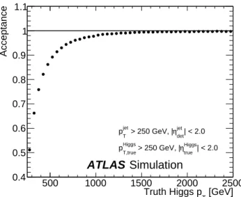
[GeV] T Truth Higgs p 500 1000 1500 2000 2500 Acceptance 0.4 0.5 0.6 0.7 0.8 0.9 1 1.1 Simulation ATLAS | < 2.0 jet det η > 250 GeV, | jet T p | < 2.0 Higgs true η > 250 GeV, | Higgs T,true p
Figure 1: Fraction of Higgs bosons in simulation which are reconstructed and labelled as a Higgs-jet following the definition in Section4, as a function of Higgs boson pT. Only Higgs bosons with pT> 250 GeV, |η| < 2.0 and with associated b-hadrons from its decay are considered. Same pTand η requirements are applied to the Higgs-jets.
6 Higgs-jet tagger
The Higgs-jet tagger algorithm consists of several reconstruction steps. First, the Higgs boson candidate is reconstructed as a large-R jet. Second, the b-tagging requirement is applied to track-jets associated with the large-R jet in order to select candidates corresponding to H → b ¯b decays. Third, the b-tagged large-R jet mass can be required to be around the SM Higgs boson mass of 125 GeV. Finally, a requirement on other large-R jet substructure variables can be applied depending on the Higgs-jet tagger working point. The signal acceptance for the first reconstruction step where the Higgs boson candidate is reconstructed as a large-R jet depends strongly on its transverse momentum. The angular separation between Higgs boson decay products can be approximated as ∆R ≈ 2mH/pT. Therefore, in most of the cases the Higgs
boson decay products will fall within a single large-R jet with a radius parameter of R = 1.0 if the Higgs boson pTis at least 250 GeV. The signal acceptance shown in Figure1is determined as the fraction of
Higgs bosons in simulation which are reconstructed and labelled as a Higgs-jet following the definition in Section4. Only Higgs bosons with pT> 250 GeV, |η| < 2.0, and associated b-hadrons from its decay that
have pT > 5 GeV and |η| < 2.5 are considered. The Higgs boson acceptance is around 50% at 250 GeV,
where the jet pT resolution have a significant impact as well, and increases to 95% for transverse momenta
above 750 GeV.
The Higgs-jet tagging efficiency is defined as the number of Higgs-jets passing a given selection requirement divided by the total number of Higgs-jets. The background rejection is defined as the inverse of the efficiency for a background jet to pass the given selection requirement.
6.1 Two-step sample reweighting
To construct the signal sample, all graviton samples are combined. To allow a valid comparison between the signal efficiency and the background rejection, the large-R jet pTspectrum of the combined graviton
sample is reweighted to the reconstructed multijet pTspectrum for the Higgs boson tagger performance
studies in a two-step procedure. The same two-step reweighting procedure is also applied to the Z0→ t ¯t background sample. The multijet spectrum is chosen as a reference because of its smoothly falling pT
spectrum being representative for many analyses. During the first step of the reweighting the highest-pT
truth Higgs-jet is used, whereas for the second reweighting step the highest-pTreconstructed Higgs-jet is
used. The reconstructed Higgs-jet and the truth Higgs-jet must both contain the highest-pTHiggs boson to
mitigate effects from initial-state radiation (ISR).
In the first step, the pT spectrum of the truth Higgs-jet in the combined signal sample is reweighted to the
pTspectrum of the reconstructed large-R jet in the multijet sample. In the second step, the reconstructed Higgs-jet pTspectrum is reweighted to the reconstructed large-R jet pTspectrum in the multijet sample. A
one-step reweighting using the reconstructed Higgs-jet pTspectrum results in large weights for jets with pT
much larger or smaller than half of the graviton mass. Furthermore, the reconstructed Higgs-jet can contain additional energy which does not stem from the Higgs boson decay, such as ISR, energy missing due to neutrinos, ‘out-of-cone’ effects, or trimming. The frequency of these effects depends on the Higgs boson boost, i.e. on the graviton mass, introducing a dependence on the choice of simulated graviton masses used in the combined signal sample. The second step is needed to account for a residual difference between reconstructed and truth Higgs-jet transverse momenta.
6.2 Flavour-tagging working points
To apply b-tagging to identify H → b ¯b decays, the track-jets are matched to the large-R jets by ghost association as described in Section4. At least two track-jets must be matched to the large-R jet for the double-b-tagging benchmarks, and at least one track-jet in the case of single-b-tagging benchmarks. The track-jet is considered to be b-tagged if its MV2c10 b-tagging discriminant value is larger than a given threshold value. These threshold values are defined for several b-tagging working points: 60%, 70%, 77% and 85% b-jet tagging efficiencies.
The following b-tagging benchmarks are studied:
• double b-tagging: the two highest-pTtrack-jets must both pass a given b-tagging requirement;
• asymmetric b-tagging: the track-jet which is more consistent with the interpretation of being a b-jet must pass a given fixed 60%, 70%, 77%, or 85% working point, while the b-tagging requirement on the second track-jet is varied;
• single b-tagging: at least one of the two highest-pTtrack-jets must pass the b-tagging requirement;
• leading single b-tagging: the highest-pTtrack-jet must pass the b-tagging requirement.
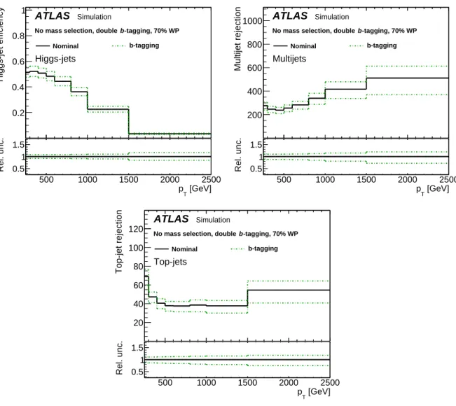
The Higgs-jet efficiencies and background rejections as a function of the jet pTfor the 70% double-b-tagging
benchmark are shown in Figure2. The signal efficiency varies from 52% at low pT to about 5% for
1500 < pT < 2500 GeV. The drop in efficiency at high transverse momenta due to the increasing collimation
and eventual merging of the two b-jets can be partially recovered using single-b-tagging working points as indicated in Figure6. The multijet (top-jet) rejection is relatively constant over the whole pTrange and is
about 250 (60) at low pTand 500 (50) at high pT.
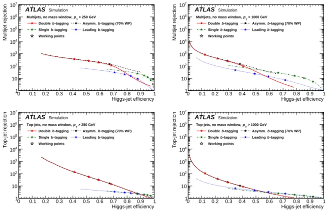
The multijet and top-quark background rejections as a function of the Higgs tagging efficiency for various b-tagging benchmarks are shown in Figure3. Plots on the left show the performance for Higgs-jet pT
[GeV] T p Higgs-jet efficiency 0.2 0.4 0.6 0.8 1 -tagging, 70% WP b
No mass selection, double
Nominal b-tagging Higgs-jets ATLAS Simulation [GeV] T p 500 1000 1500 2000 2500 Rel. unc. 0.5 1 1.5 [GeV] T p Multijet rejection 200 400 600 800 1000 -tagging, 70% WP b
No mass selection, double
Nominal b-tagging Multijets ATLAS Simulation [GeV] T p 500 1000 1500 2000 2500 Rel. unc. 0.5 1 1.5 [GeV] T p Top-jet rejection 20 40 60 80 100
120 No mass selection, double b-tagging, 70% WP
Nominal b-tagging Top-jets ATLAS Simulation [GeV] T p 500 1000 1500 2000 2500 Rel. unc. 0.5 1 1.5
Figure 2: The Higgs-jet efficiency (top left) and rejection against multijet (top right) and top-jet backgrounds (bottom) as a function of the jet pTfor the 70% double-b-tagging working point. The nominal curves correspond to the requirement on the MV2c10 discriminant described in Section6.2. The b-tagging-related uncertainties defined in Section5are shown.
Higgs-jet efficiency 0 0.1 0.2 0.3 0.4 0.5 0.6 0.7 0.8 0.9 1 Multijet rejection 1 10 2 10 3 10 4 10 5 10 6 10 7 10 > 250 GeV T p
Multijets, no mass window, -tagging
b
Double Asymm. b-tagging (70% WP) -tagging
b
Single Leading b-tagging Working points ATLAS Simulation Higgs-jet efficiency 0 0.1 0.2 0.3 0.4 0.5 0.6 0.7 0.8 0.9 1 Multijet rejection 1 10 2 10 3 10 4 10 5 10 6 10 7 10 > 1000 GeV T p
Multijets, no mass window, -tagging
b
Double Asymm. b-tagging (70% WP) -tagging
b
Single Leading b-tagging Working points ATLAS Simulation Higgs-jet efficiency 0 0.1 0.2 0.3 0.4 0.5 0.6 0.7 0.8 0.9 1 Top-jet rejection 1 10 2 10 3 10 4 10 5 10 6 10 7 10 > 250 GeV T p
Top-jets, no mass window, -tagging
b
Double Asymm. b-tagging (70% WP) -tagging
b
Single Leading b-tagging Working points ATLAS Simulation Higgs-jet efficiency 0 0.1 0.2 0.3 0.4 0.5 0.6 0.7 0.8 0.9 1 Top-jet rejection 1 10 2 10 3 10 4 10 5 10 6 10 7 10 > 1000 GeV T p
Top-jets, no mass window, -tagging
b
Double Asymm. b-tagging (70% WP) -tagging
b
Single Leading b-tagging Working points
ATLAS Simulation
Figure 3: The multijet (top) and the top-jet (bottom) rejection as a function of the Higgs tagging efficiency for large-R jet pTabove 250 GeV (left) and above 1000 GeV (right) for various b-tagging benchmarks defined in Section6.2. The stars correspond to the 60%, 70%, 77% and 85% b-tagging WPs (from left to right). The curves for the double-b-tagging and asymmetric-b-tagging working points coincide over a large range of Higgs-jet efficiency.
above 250 GeV and plots on the right show the performance for Higgs-jet pT above 1000 GeV. The
double-b-tagging and asymmetric-b-tagging selections give the best background rejection in a large range of Higgs tagging efficiencies. At high Higgs-jet efficiencies above ∼90% (∼55%) for Higgs-jet transverse momenta above 250 (1000) GeV the single-b-tagging benchmark shows a higher multijet and top-quark background rejection. To achieve such a high Higgs-jet efficiency, a very loose double-b-tagging or asymmetric-b-tagging requirement is needed, which results in a low light-flavour jet rejection. The double-b-tagging and asymmetric b-tagging working points do not reach an efficiency of 100% due to a requirement of at least two track-jets. In the case of asymmetric b-tagging, Higgs tagging efficiencies are below 100% because of the fixed b-tagging working point requirement on one of the track-jets. The drop in performance is pronounced at high jet transverse momenta due to the lower efficiency to reconstruct two subjets and the decrease in the MV2c10 b-tagging performance [64].
6.3 Mass window optimisation
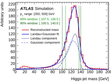
The reconstructed Higgs boson mass distribution provides a powerful way to distinguish the Higgs boson signal from background processes. The muon-corrected combined mass described in Section4is used to impose the Higgs boson mass requirement and select large-R jets with a mass around the SM Higgs boson mass. The Higgs boson mass resolution, σm, varies as a function of the reconstructed large-R jet pT, so
0 20 40 60 80 100 120 140 160 180 200 Higgs-jet mass [GeV] 0 20 40 60 80 100 120 140 160 180 200 220 Arbitrary units Simulation ATLAS range: [350, 500] GeV T p 68% window: [ 107.5, 136.5 ] 80% window: [ 100.5, 140.0 ] Reconstructed mass Landau+Gaussian fit Landau component Gaussian component
Figure 4: The Higgs-jet mass distribution for jet transverse momenta in the range 350 to 500 GeV after reweighting the pTspectrum. The dotted and dash-dotted blue curves correspond to the two components of the fit function, while the solid blue curve shows the combination thereof. The vertical lines indicate the boundaries of the mass ranges for 68% (light green) and 80% (dark green) containment.
the mass window is optimised and parameterised as a function of Higgs-jet pT. Two working points are
defined:
• tight mass window, containing 68% of Higgs-jets; • loose mass window, containing 80% of Higgs-jets.
The mass window is defined as the smallest window containing the given fraction of Higgs-jets. The out-of-cone effects, ISR and the missing neutrinos from semileptonic b-hadron decays have an impact on the mass resolution that is similar to their impact on the pT response; therefore, the mass window
optimisation depends on the applied Higgs-jet selection and on the Higgs-jet pTspectrum.
Figure4shows the reconstructed Higgs boson mass distribution for Higgs-jets with a pTin the range 350
to 500 GeV. The mass region below 50 GeV is affected by grooming and out-of-cone effects. In the case of asymmetric H → b ¯b decays, where one of the b-hadrons carries a large fraction of the Higgs boson pT, the
large-R jet’s axis is close to the direction of the higher-pTb-hadron. The decay products of the lower-pT
b-hadron could be removed by grooming or not fully captured in the large-R jet. That leads to smaller Higgs-jet masses. The mass region above 150 GeV suffers from additional contributions from initial-state radiation. A large fraction of the ISR is suppressed by selecting the reconstructed Higgs-jet containing the highest-pTHiggs boson candidate. However, the high mass tails are still substantial in high Higgs-jet pT
regions and affect the Higgs boson mass window definition.
In order to suppress the impact of the tails on the mass window definition, a fit of the mass distribution is performed. The fit function is chosen empirically to describe the core of the mass distribution, while mitigating the tails. The chosen function is a linear combination of a Landau function to describe the low mass part of the distribution and a Gaussian function to describe the high mass part.
The fit is performed in 12 Higgs-jet pTbins across the entire range of transverse momentum from 250 to
500 1000 1500 2000 2500 [GeV] T p 80 100 120 140 160 180 200 mass [GeV] Simulation ATLAS
Mass window for 80% working point
500 1000 1500 2000 2500 [GeV] T p 80 100 120 140 160 180 200 mass [GeV] Simulation ATLAS
Mass window for 68% working point
Figure 5: The Higgs-jet mass window interval for a loose (left) and a tight (right) working point. The dashed lines show a fit to the derived intervals (blue and red markers) as a function of the Higgs-jet pT. The black markers show the position of the maximum of the Higgs-jet mass distribution.
A toy MC simulation is used as input to model the mass window and to estimate the statistical uncertainty on the mass window determination. This toy MC simulation samples the fit functions mentioned above and is performed many times in each pT slice. For each toy MC sample, the mass window is calculated by
selecting the smallest window containing the required signal fraction. The final upper and lower boundaries for a given pTslice are found by averaging over the upper and lower boundaries from the corresponding toy
MC samples. The mean defines the position and the RMS the uncertainty of the window boundaries in each pTslice. Using the mean and RMS from the toy MC samples as input, the mass window is parameterised as a function of the Higgs-jet pT using the fit function: f (pT) =
q
(a+ b/pT)2+ (c · p
T+ d)2. The jet
mass depends primarily on the energies of the jet constituents and their angular separations. Consequently, there are two competing effects: the improving precision of the calorimeter energy scale with increasing jet pTand the decreasing ability of the calorimeter granularity to resolve individual energy deposits due to
increasing decay collimation with increasing jet pT. Fit results are shown in Figure5for tight and loose
mass window working points.
The Higgs boson acceptance times efficiency is presented in Figure6. In addition to the truth-matching requirements defined for Figure1, the double- and single-b-tagging, tight, loose and no mass window working points are applied. The double-b-tagging requirement in particular leads to a significant drop in the Higgs boson acceptance times efficiency at high Higgs boson transverse momenta, where the efficiency to reconstruct two track-jets and the double-b-tagging efficiency decrease quickly.
Figure7shows the rejection of the multijet background as a function of the Higgs-jet pT. Applying a
combination of loose mass window and double-b-tagging requirements improves the rejection by a factor of about four relative to the corresponding benchmark without the mass requirement shown in Figure2. The tight mass window requirement leads to an additional improvement of about 30–50% in the background rejection. The efficiency of the mass window requirements changes by a few percent after the application of the double b-tagging-requirement due to the dependence of the b-tagging efficiency on the jet kinematics. The corresponding rejection of the multijet background as a function of the Higgs-jet efficiency is shown in Figure8 for different Higgs-jet pT ranges, b-tagging benchmarks, and mass window requirements.
Application of the mass window requirement improves the performance of the tagger substantially. For a fixed signal efficiency of 40% and large-R jet pT above 250 GeV, the multijet rejection rises from roughly
[GeV] T Truth Higgs p 500 1000 1500 2000 2500 efficiency × Acceptance 0 0.1 0.2 0.3 0.4 0.5 0.6 0.7 0.8 0.9 1
1 b-tag, loose mass window 2 b-tags, no mass selection 2 b-tags, loose mass window 2 b-tags, tight mass window
Simulation ATLAS MV2c10 b-tagging at 70% WP | < 2.0 jet det η > 250 GeV, | jet T p | < 2.0 Higgs true η > 250 GeV, | Higgs T,true p
Figure 6: The Higgs boson acceptance times efficiency is shown for a few working points: the double and single b-tagging with the loose mass window requirement and the double b-tagging with the tight, loose and no mass window requirements. [GeV] T p Multijet rejection 1000 2000 3000 4000 5000 6000 7000 8000 9000 -tagging, 70% WP b
Loose mass window, double
Nominal Jet Scale b-tagging Jet Resolution Total syst. uncert.
Multijets ATLAS Simulation [GeV] T p 500 1000 1500 2000 2500 Rel. unc. 0.5 1 1.5 [GeV] T p Multijet rejection 2 4 6 8 10 12 3 10 × -tagging, 70% WP b
Tight mass window, double
Nominal Jet Scale b-tagging Jet Resolution Total syst. uncert.
Multijets ATLAS Simulation [GeV] T p 500 1000 1500 2000 2500 Rel. unc. 0.5 1 1.5
Figure 7: Rejection of multijet background as a function of the Higgs-jet pTfor the loose (left) and tight (right) mass window requirements, in combination with the 70% double-b-tagging working point. The nominal curves correspond to the requirement on the MV2c10 discriminant described in Section6.2. Systematic uncertainties defined in Section5as well as their sum in quadrature (total uncertainty) are shown. ‘Jet Scale’ refers to the sum in quadrature of the jet energy and mass scale uncertainties and ‘Jet Resolution’ refers to the sum in quadrature of the jet energy and mass resolution uncertainties.
Higgs-jet efficiency 0 0.1 0.2 0.3 0.4 0.5 0.6 0.7 0.8 0.9 1 Multijet rejection 1 10 2 10 3 10 4 10 5 10 6 10 7 10 > 250 GeV T p
Multijets, loose mass window, -tagging
b
Double Asymm. b-tagging (70% WP) -tagging
b
Single Leading b-tagging Working points ATLAS Simulation Higgs-jet efficiency 0 0.1 0.2 0.3 0.4 0.5 0.6 0.7 0.8 0.9 1 Multijet rejection 1 10 2 10 3 10 4 10 5 10 6 10 7 10 > 1000 GeV T p
Multijets, loose mass window, -tagging
b
Double Asymm. b-tagging (70% WP) -tagging
b
Single Leading b-tagging Working points ATLAS Simulation Higgs-jet efficiency 0 0.1 0.2 0.3 0.4 0.5 0.6 0.7 0.8 0.9 1 Multijet rejection 1 10 2 10 3 10 4 10 5 10 6 10 7 10 > 250 GeV T p
Multijets, tight mass window, -tagging
b
Double Asymm. b-tagging (70% WP) -tagging
b
Single Leading b-tagging Working points ATLAS Simulation Higgs-jet efficiency 0 0.1 0.2 0.3 0.4 0.5 0.6 0.7 0.8 0.9 1 Multijet rejection 1 10 2 10 3 10 4 10 5 10 6 10 7 10 > 1000 GeV T p
Multijets, tight mass window, -tagging
b
Double Asymm. b-tagging (70% WP) -tagging
b
Single Leading b-tagging Working points
ATLAS Simulation
Figure 8: Rejection of multijet background as a function of the Higgs boson tagging efficiency for loose (top) and tight (bottom) mass window requirements for large-R jet pTabove 250 GeV (left) and above 1000 GeV (right) for various b-tagging benchmarks. The stars correspond to the 60%, 70%, 77% and 85% b-tagging WPs (from left to right). The curves for the double- and asymmetric-b-tagging working points coincide over a large range of Higgs-jet efficiency.
360 after applying the double-b-tagging requirement to about 1480 (1670) for the combination of the double-b-tagging and loose (tight) mass window requirements.
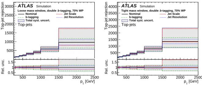
Figure 9 shows the hadronic top-quark background rejection as a function of the Higgs-jet pT for
combinations of mass window and b-tagging benchmarks. The background rejection is higher for multijets than for hadronically decaying top quarks. The rejection varies between 120 (170) at low pT and 1000
(1300) at high pTfor the loose (tight) mass window and double-b-tagging benchmark. In comparison with
the benchmarks without the mass window requirement, the rejection is improved by about one order of magnitude, but the shape as function of pTis fundamentally different. At low pT, not all decay products of
the top quark are contained in the large-R jet. Thus the reconstructed jet mass has a long tail towards low jet masses with a substantial fraction of jets within the mass window of the tagger. Hence, the rejection at low jet pTis not improved as much as at high jet pT. The tight mass window requirement further improves
the background rejection by 15–40% as function of pT.
The rejection of the hadronic top-quark background as a function of the Higgs tagging efficiency is shown in Figure10. For the loose mass window requirement, an improvement from 140 to 200 is found at a fixed Higgs-jet efficiency of 40%, whereas for the tight mass window a smaller improvement from 140 to 160 is observed relative to no mass requirement for large-R jet pTabove 250 GeV. The rejection values are lower
for double b-tagging and asymmetric b-tagging for large-R jet pTabove 1 TeV, and for high Higgs tagging
[GeV] T p Top-jet rejection 500 1000 1500 2000 2500 3000 -tagging, 70% WP b
Loose mass window, double
Nominal Jet Scale b-tagging Jet Resolution Total syst. uncert.
Top-jets ATLAS Simulation [GeV] T p 500 1000 1500 2000 2500 Rel. unc. 0.5 1 1.5 [GeV] T p Top-jet rejection 500 1000 1500 2000 2500 3000 3500 4000 -tagging, 70% WP b
Tight mass window, double
Nominal Jet Scale b-tagging Jet Resolution Total syst. uncert.
Top-jets ATLAS Simulation [GeV] T p 500 1000 1500 2000 2500 Rel. unc. 0.5 1 1.5
Figure 9: Rejection of the top-jet background as a function of the Higgs-jet pTfor the loose (left) and tight (right) mass window requirements, in combination with the 70% double-b-tagging working point. The nominal curves correspond to the requirement on the MV2c10 discriminant described in Section6.2. Systematic uncertainties defined in Section5as well as their sum in quadrature (total uncertainty) are shown. ‘Jet Scale’ refers to the sum in quadrature of the jet energy and mass scale uncertainties and ‘Jet Resolution’ refers to the sum in quadrature of the jet energy and mass resolution uncertainties.
Higgs-jet efficiency 0 0.1 0.2 0.3 0.4 0.5 0.6 0.7 0.8 0.9 1 Top-jet rejection 1 10 2 10 3 10 4 10 5 10 6 10 7 10 > 250 GeV T p
Top-jets, loose mass window, -tagging
b
Double Asymm. b-tagging (70% WP) -tagging
b
Single Leading b-tagging Working points ATLAS Simulation Higgs-jet efficiency 0 0.1 0.2 0.3 0.4 0.5 0.6 0.7 0.8 0.9 1 Top-jet rejection 1 10 2 10 3 10 4 10 5 10 6 10 7 10 > 1000 GeV T p
Top-jets, loose mass window, -tagging
b
Double Asymm. b-tagging (70% WP) -tagging
b
Single Leading b-tagging Working points ATLAS Simulation Higgs-jet efficiency 0 0.1 0.2 0.3 0.4 0.5 0.6 0.7 0.8 0.9 1 Top-jet rejection 1 10 2 10 3 10 4 10 5 10 6 10 7 10 > 250 GeV T p
Top-jets, tight mass window, -tagging
b
Double Asymm. b-tagging (70% WP) -tagging
b
Single Leading b-tagging Working points ATLAS Simulation Higgs-jet efficiency 0 0.1 0.2 0.3 0.4 0.5 0.6 0.7 0.8 0.9 1 Top-jet rejection 1 10 2 10 3 10 4 10 5 10 6 10 7 10 > 1000 GeV T p
Top-jets, tight mass window, -tagging
b
Double Asymm. b-tagging (70% WP) -tagging
b
Single Leading b-tagging Working points
ATLAS Simulation
Figure 10: Rejection of the top-jet background as a function of the Higgs tagging efficiency for loose (top) and tight (bottom) mass window requirements for large-R jet pTabove 250 GeV (left) and above 1000 GeV (right) for various b-tagging benchmarks. The stars correspond to the 60%, 70%, 77% and 85% b-tagging WPs (from left to right). The curves for the double- and asymmetric-b-tagging working points coincide over a large range of Higgs-jet efficiency.
Table 1: Overview of jet substructure variables. A short description of these substructure variables can be found in Refs. [65,66].(∗)Exclusive dipolarity forces the jet to have exactly two subjets from the ktalgorithm to begin with, which is different from the dipolarity, which runs ktclustering and then takes all jets with pTabove 5 GeV.
Symbol Description Reference
Energy correlation functions
ECFi i-th energy correlation function [67,68] Cβ=1 2 ECF3· ECF1/ECF2 Dβ=1 2 ECF3· (ECF1/ECF2) 3 n-subjettiness τn n-subjettiness [69,70] τwta
n n-subjettiness variant winner takes all (wta)
τji, τwtaji τj/τior τwtaj /τiwta, j > i
Centre-of-mass observables
Fi i-th Fox–Wolfram moment [71]
Dipolarity
Dexcl Exclusive dipolarity(∗) [72]
Cluster sequence
kt∆R ∆R of two subjets within the large-R jet [46]
µ12 ktmass drop [11]
Splitting measures
pdi j ktsplitting scale from i → j splitting [73,74] Thrust
Tmin, Tmax Thrust [75]
Shape A Aplanarity [76] P Planar flow [77] S Sphericity [76] Other a3 Angularity [78] 6.4 Jet substructure
Sections6.2and6.3present the performance of the Higgs-jet tagger based on the b-tagging and jet mass requirements designed to distinguish large-R jets produced by Higgs boson decays from backgrounds. This section discusses the possibility of improving the background rejection with the help of other jet substructure variables and tighter selections on jet mass and b-tagging applied on top of the previously defined jet mass window and b-tagging benchmark working points. These additional selections are referred to as secondary selections.
Many jet substructure variables exist that can capture features of a jet’s internal structure and can potentially give additional discrimination power against backgrounds from multijet production and top-quark decays. They are based on the jet constituents and exploit quantities such as transverse momentum and angular distance between the constituents. They give information about different jet attributes such as shape (e.g.
0 0.02 0.04 0.06 0.08 0.1 0.12 0.14 0.16 ) | JSS v, corr m( C Correlation | single b-tagging > 250 GeV T p double b-tagging > 250 GeV T p single b-tagging > 1000 GeV T p double b-tagging > 1000 GeV T p Mass double b-tagging single b-tagging 0 F / 1 F
Fox Wolfram ratio 0
F
/ 4
F
Fox Wolfram ratio 0
F
/ 3
F
Fox Wolfram ratio 0
F
/ 2
F
Fox Wolfram ratio =1 β 2 C min Thrust T ) P ( log Planar Flow 21 τ =1 β 2 D 0.03 ± 1.80 0.12 ± 3.62 0.03 ± 2.13 0.03 ± 1.55 0.03 ± 1.97 0.04 ± 1.81 0.03 ± 1.93 0.02 ± 1.79 0.03 ± 1.94 0.03 ± 1.84 0.03 ± 1.99 0.04 ± 2.09 0.10 ± 1.93 0.06 ± 1.35 0.06 ± 1.36 0.07 ± 1.42 0.10 ± 1.83 0.09 ± 1.68 0.09 ± 1.81 0.09 ± 1.62 0.09 ± 1.79 0.08 ± 1.71 0.09 ± 1.77 0.11 ± 1.87 0.04 ± 1.60 0.13 ± 1.29 0.02 ± 1.96 0.02 ± 1.97 0.02 ± 1.59 0.04 ± 1.90 0.02 ± 1.78 0.04 ± 2.10 0.02 ± 1.83 0.05 ± 2.03 0.02 ± 1.99 0.02 ± 2.12 0.08 ± 1.69 0.04 ± 1.37 0.04 ± 1.46 0.06 ± 1.79 0.05 ± 1.62 0.08 ± 1.86 0.06 ± 1.81 0.07 ± 1.89 0.06 ± 1.82 0.09 ± 2.01 0.06 ± 1.94 0.08 ± 2.08
ATLAS
Simulation
=80% S εAdditional multijet background rejection at Flavour tagging WP 70%, loose mass window
Figure 11: Multijet background rejection at 80% signal efficiency (εS= 80%) for a variety of substructure variables using different benchmarks in terms of b-tagging strategy and transverse momentum range. The z-axis colour scale represents the absolute value of the linear-correlation coefficient, |C(mcorr, vJSS)|, between the jet mass and the jet substructure variables. The selection efficiency is determined relative to the mass window and b-tagging benchmark working points defined in Sections6.3and6.2respectively.
sphericity, aplanarity) or number of axes (e.g. two-subjettiness τ2). Ratios are often used to avoid scale
dependence of substructure variables. Table1lists the jet substructure variables that are investigated in this study, together with a short description and references. Secondary selections on jet mass and the flavour-tagging discriminant for the track-jets, MV2c10, are also considered relative to the previously defined mass window and b-tagging benchmark working points and their performance is compared with that achieved by the application of additional jet substructure variables to these benchmarks. Two categories of secondary selections are used for the b-tagging discriminant MV2c10, and these exploit the potential of tighter b-tagging working points where the criteria are tightened for both track-jets (double b-tagging) or for only one track-jet (single b-tagging).
For all secondary selection variables an optimal two-sided range is chosen for each variable and each benchmark working point. Searches of new-physics resonances typically use tagging definitions with relatively high signal efficiency, around 40% (75%) for Higgs-jets with pT = 500 GeV for double (single)
b-tagging and a mass requirement. Hence, the two-sided range for a secondary variable which contains the smallest fraction of background but at least 80% of signal events is determined. Figures11and12show the background rejection for a 80% retention of signal efficiency relative to the jet mass and b-tagging benchmark working points for multijet and hadronic top-quark backgrounds, respectively. The matrices in Figures11and12show the background rejection for substructure variables, secondary jet mass, and MV2c10 b-tagging discriminant on the y-axis for the four benchmark points of the Higgs-jet tagger on
0 0.05 0.1 0.15 0.2 0.25 0.3 0.35 ) | JSS v, corr m( C Correlation | single b-tagging > 250 GeV T p double b-tagging > 250 GeV T p single b-tagging > 1000 GeV T p double b-tagging > 1000 GeV T p Mass double b-tagging single b-tagging R ∆ T k max Thrust T 1 F / 4 F
Fox Wolfram ratio ) S ( log Sphericity 0 F / 4 F
Fox Wolfram ratio 0
F
/ 2
F
Fox Wolfram ratio min Thrust T ) excl 12 D ( log Exclusive Dipolarity 0.03 ± 1.59 0.19 ± 4.81 0.01 ± 1.51 0.01 ± 1.24 0.04 ± 1.43 0.01 ± 1.48 0.01 ± 1.45 0.01 ± 1.46 0.01 ± 1.44 0.01 ± 1.46 0.01 ± 1.47 0.07 ± 1.60 0.10 ± 2.34 0.06 ± 1.70 0.04 ± 1.29 0.05 ± 1.43 0.06 ± 1.48 0.05 ± 1.47 0.05 ± 1.51 0.05 ± 1.46 0.06 ± 1.49 0.06 ± 1.51 0.03 ± 1.53 0.11 ± 1.18 0.01 ± 1.54 0.02 ± 1.41 0.02 ± 1.56 0.02 ± 1.57 0.02 ± 1.57 0.02 ± 1.59 0.02 ± 1.58 0.02 ± 1.60 0.03 ± 1.59 0.08 ± 1.60 0.07 ± 1.57 0.07 ± 1.71 0.10 ± 1.81 0.08 ± 1.79 0.08 ± 1.67 0.08 ± 1.73 0.08 ± 1.71 0.09 ± 1.84 0.08 ± 1.80 0.08 ± 1.84
ATLAS
Simulation
=80% S εAdditional top-jet background rejection at Flavour tagging WP 70%, loose mass window
Figure 12: Hadronic top-quark background rejection at 80% signal efficiency (εS= 80%) for a variety of substructure variables using different benchmarks in terms of b-tagging strategy and transverse momentum range. The z-axis colour scale represents the absolute value of the linear-correlation coefficient, |C(mcorr, vJSS)|, between the jet mass and the jet substructure variables. The selection efficiency is determined relative to the mass window and b-tagging benchmark working points defined in Sections6.3and6.2respectively.
the x-axis. The z-axis colour scale represents the absolute value of the linear-correlation coefficient of the substructure variable and the jet mass for the corresponding background. For each benchmark, five variables with the largest background rejection are selected and all selected variables for every benchmark are shown.
In general, there are improvements across the various benchmark points. The background rejection is often higher for the multijet background than for the hadronically decaying top quarks. The secondary b-tagging discriminant is very powerful, and there are only a few areas of phase space where substructure yields larger improvements than an optimised b-tagging working point. However, substructure variables are an interesting alternative to tighter b-tagging working points for large-R jet pTabove 1 TeV. For the multijet
background (Figure11), a tighter requirement on the double b-tagging achieves a background rejection of 3.62 (1.35) in the inclusive range pT > 250 GeV for the single-b-tagging (double-b-tagging) working
point. In contrast, the improvement from the double-b-tagging discriminant is small for working points for pT> 1000 GeV, achieving a background rejection of 1.29 (1.37) for the single-b-tagging (double-b-tagging) working point. At large pTthe background rejection for substructure variables varies between 2.12 (D
β=1
2 )
and 1.55 (Fox–Wolfram ratio F1/F0) for a signal efficiency of 80%. In general, correlations with the jet
mass greater than 10% are observed for most of the jet substructure variables. The Fox–Wolfram ratios F3/F0and F1/F0show the lowest correlations: less than 1% for most of the benchmarks.
and b-tagging benchmark working points are used in the case of the hadronic top-quark background (Figure12). A tighter double-b-tagging working point reaches a factor of 4.81 (2.34) background rejection in the inclusive range pT > 250 GeV for the single-b-tagging (double-b-tagging) working point. In contrast,
the improvement from the double-b-tagging discriminant is small at large pT, achieving a background
rejection of 1.18 (1.57) for the single-b-tagging (double-b-tagging) working point. The background rejection for other variables varies between 1.84 (Fox–Wolfram ratio F2/F0 and exclusive dipolarity)
and 1.24 (kt∆R) for a signal efficiency of 80%. Compared with the multijet background the correlations
between the jet mass and the jet substructure variables are smaller in the case of the top-quark background, especially for pT > 1000 GeV. The Fox–Wolfram ratio F4/F1shows the lowest correlation: less than 1%
for most of the benchmarks.
In conclusion, the application of jet substructure variables improves the background rejection moderately, while better improvements are observed for high transverse momenta. Furthermore, it is important to take into account the correlation between the large-R jet mass and the substructure variables since requirements on the substructure variables sculpt the jet mass distribution [79,80].
7 Modelling tests in
g → b ¯
b data
Multijet events enriched in b-jets, which predominately originate from gluon to b ¯b production, are used to evaluate the b-tagging efficiency in data and simulation as well as the modelling of jet substructure variables. The multijet background is one of the main backgrounds for searches in fully hadronic final states, for example the Higgs boson pair search in the four-b-quark final state [81]. This background also provides a unique opportunity to validate the modelling of the double-b-jets in a large data sample. Events with one large-R jet with two ghost-associated track-jets (‘g → b ¯b candidate jet’) and one recoiling ISR small-R jet (‘recoil jet’, jrecoil) are used for this study.
7.1 Event selection
Events are required to have a primary vertex that has at least two tracks, each with pT > 500 MeV [82].
The primary vertex with the highest p2Tsum of associated tracks is selected. A single-small-R-jet trigger with an online ETthreshold of 380 GeV was used to collect the data. An offline R = 0.4 recoil jet with pT
above 500 GeV is matched to the jet which fired the trigger.
Non-collision backgrounds originating from calorimeter noise, beam-halo interactions, or cosmic rays can lead to spurious calorimeter signals. This effect is suppressed by applying the criteria described in Ref. [83].
Selected events are required to have at least one large-R jet with pT > 500 GeV and |η| < 2.0, for which the
small-R jet trigger is fully efficient and unbiased. The large-R jet must have at least two ghost-associated R= 0.2 track-jets. To enrich the event sample in jets containing b-hadrons, it is required that at least one of the ghost-associated track-jets be matched to a muon. The highest-pTtrack-jet matched to a muon is called
the muon-tagged jet, jµtrk. The matching is performed using a geometric ∆R < 0.2 requirement between the track-jet’s axis and the muon. The highest-pT jet among the remaining track-jets matched by ghost
association to the large-R jet is called the non-muon jet, jnon-µtrk . The highest-pTlarge-R jet satisfying these
criteria is selected as gluon-jet candidate. Furthermore, the event must satisfy ∆R( jrecoil, jµtrk)> 1.5. This
7.2 Flavour fraction corrections
To reduce discrepancies between data and MC simulation in the flavour composition of the large-R jet, the flavour fractions of the sample are determined from the data before applying b-tagging. Each large-R jet carries two flavours, that of jµtrkand jnon-µtrk , leaving nine possible flavour combinations for the large-R jet (each track-jet can be a b-jet, c-jet, or light-flavour jet; B, C and L abbreviations are used in the following). The long decay length of b- and c-hadrons makes the signed impact parameter significance, sd0, of tracks
associated with a jet a good discriminating variable for different jet flavours. The sd0of a track is defined
as:
sd
0 =
d0 σ(d0)sj,
where d0is the track’s transverse impact parameter relative to the primary vertex, σ(d0) is the uncertainty
in the d0measurement, and sjis the sign of d0relative to the track-jet’s axis, depending on whether the
track crosses the track-jet’s axis in front of or behind the primary vertex. For a given track-jet, the average sd
0
is built from the three highest-pTtracks associated with the track-jet. The tracks from b- and c-hadron
decays are expected to have higher pTthan tracks in light-flavour jets, because the heavy-flavour hadrons
carry on average a larger fraction of the jet energy. The requirement that sd0
is built from the three highest-pTtracks helps to distinguish them from light-flavour jets, which may have tracks with large sd0
values, e.g. from Λ and Ksdecays.
The impact parameter resolution depends on the intrinsic track resolution, the traversed detector material, the detector alignment, and other effects. To determine the impact parameter resolution in data, minimum-bias, dijet, and Z +jets events are used. The impact parameter resolution is extracted in fine bins of track pT
and η with an iterative method described in Ref. [51]. The simulation is corrected to match the measured impact parameter resolution as a function of track pT and η by using a Gaussian function to smear the
impact parameter resolution in the simulation. The sd0
values of jµtrk and jnon-µtrk are found to be uncorrelated and thus the one-dimensional distributions of each jet’s sd0
are fit simultaneously. Furthermore, the flavour combinations of ( jµtrk, jnon-µtrk ) = {(B,C), (C,B), (L,C), (L,B)} are predicted to be less than 1% of the total, so they are merged with other flavour categories which have the closest shape. The shape similarity is determined using the χ2-statistic. Thus a total of five flavour categories are used, ( jµtrk, jnon-µtrk ) = {(B,B), (B,L), (C,C), (C,L), (L,L)}. Figure13shows the templates inclusive in pT.
Since the flavour fractions vary with pT, the flavour fraction fits to the data are performed in bins of pTof
the two track-jets. For each jet pT bin, individual MC templates are used. The following jet-pTbins are
considered: jµtrk pT bins = {(0–100), (100–200), >200} GeV and jnon-µtrk pTbins = {(0–100), (100–200),
(200–300), >300} GeV. Figure14shows an example of the flavour fraction fit to the sd0 distributions of
jtrk
µ and jnon-µtrk for one particular bin of the track-jet transverse momenta. The fit uncertainty includes the statistical uncertainty of the templates and is evaluated using toy MC simulations. The flavour fraction corrections relative to the simulated fractions vary between 0.7 and 1.7 in the jet pTbins with a statistical
uncertainty below 10%.
After correcting for the observed flavour-pair fractions the level of agreement between data and MC simulation is evaluated in the selected event sample before and after b-tagging is applied to the track-jets. The 70% double-b-tagging working point is used.
40 − −20 0 20 40 60 80 〉 d0 s 〈 Muon jet 4 − 10 3 − 10 2 − 10 1 − 10 1 10 Normalised to unity Simulation ATLAS = 13 TeV s bb-enriched sample → g -jet µ BB BL CC CL LL 40 − −20 0 20 40 60 80 〉 d0 s 〈 Non-muon jet 3 − 10 2 − 10 1 − 10 1 10 Normalised to unity Simulation ATLAS = 13 TeV s bb-enriched sample → g -jet µ non-BB BL CC CL LL
Figure 13: Averaged impact parameter significance, sd0
, distributions for the muon (left) and non-muon jets (right) inclusive in jµtrkand jnon-µtrk transverse momenta. The double flavour labels denote the true flavour of the jet pair, with the jµtrkgiven first.
10 2 10 3 10 4 10 5 10 6 10 Events LL CL CC BL BB Data ATLAS -1 =13 TeV, 36.1 fb s bb-enriched sample → g -jet µ 40 − −20 0 20 40 60 80 〉 d0 s 〈 Muon jet 0.5 1 1.5 Data/MC 10 2 10 3 10 4 10 5 10 6 10 Events LL CL CC BL BB Data ATLAS -1 =13 TeV, 36.1 fb s bb-enriched sample → g -jet µ non-40 − −20 0 20 40 60 80 〉 d0 s 〈 Non-muon jet 0.5 1 1.5 Data/MC
Figure 14: Averaged impact parameter significance, sd0 , distributions of the muon (left) and non-muon jet (right) in the (100–200) GeV bin of the jµtrkand jnon-µtrk transverse momenta.
7.3 b-tagging results
Since the flavour fractions are corrected in the MC simulation, differences between the data and predictions after the b-tagging can be attributed to a difference between data and MC simulation in the dependence of the b-tagging performance on the large-R jet topology, in particular on the topology with two closely spaced track-b-jets.
Figure15shows the flavour-fit-corrected pT spectrum of the large-R jet as well the jµtrkand jnon-µtrk before
and after b-tagging. As seen in the ratio plots, there is good agreement within uncertainties between data and MC simulation. The shape differences between data and MC simulations especially for the jtrk
non-µtransverse momentum can be partially explained by the difference observed between Pythia8 and
Herwig++ MC simulations. The double-b-tagging rate is defined as the number of selected large-R jets with at least two track-jets, two of which are b-tagged, divided by the number of all selected large-R jets with at least two track-jets. Figure16shows the double-b-tagging rate as a function of the large-R jet pT.
Data and MC simulation agree within the uncertainties. The performance of the double b-tagging applied to two track-jets seems not to depend on the large-R jet topology with two closely spaced track-b-jets, and the default b-tagging calibration described in Section5can be applied for this analysis.
7.4 Jet substructure results
As possible variations of Higgs taggers may make use of the large-R jet pT, and substructure variables
such as mass, n-subjettiness, or D2β=1, it is important to ensure that these variables are well modelled by MC simulations. The distributions of kinematic and substructure variables are shown in Figure17, for double-b-tagged jets after the flavour-fit correction. As seen in the ratio plots, there is acceptable agreement within uncertainties between data and MC simulations.
The relative impact of the systematic uncertainties on the yields of signal and background are presented in Table2. The dominant signal uncertainty is the modelling uncertainty followed by the b-tagging-related uncertainties. The b-tagging-related uncertainties (misidentification of light-flavour jets and c-jets as b-jets) are dominant for background. The dominant uncertainties are shown separately in Figure17. The difference in the shapes between data and MC simulations can be partially explained by the difference observed between Pythia8 and Herwig++ MC simulations.
Table 2: Relative impact of the systematic uncertainties on the yields of signal and the main background for the g → b ¯b analysis. Multiple independent components have been combined into groups of systematic uncertainties. ‘Jet scales’ refers to the sum in quadrature of the jet energy, mass and substructure scale uncertainties.
Source Signal (B,B) [%] Background (non-B,non-B) [%]
Jet scales 9.0 7.3
Jet energy resolution 1.0 1.8
Jet mass resolution 0.1 0.2
JVT 0.01 0.01
b-tagging related 9.5 27
Modelling 23 13