Decomposition And Particle Motion Of The Acoustic Dipole Log In Anisotropic Formation

ACOUSTIC DIPOLE LOG IN ANISOTROPIC

FORMATION

Ningya Cheng and C. H. Cheng

Earth Resources Laboratory

Department of Earth, Atmospheric, and Planetary Sciences Massachusetts Institute of Technology

Cambridge, MA 02139

ABSTRACT

For linear wave propagation in anisotropic media, the principle of superposition still holds. The decomposition of the acoustic dipole log is based on this principle. In the forward decomposition inline and crossline acoustic dipole logs at any azimuthal an-gle the projection of measurements is along the principal direction of the formation. In the inverse decomposition the measurements along the principal direction can be constructed from the orthogonal pair of inline and crossline acoustic dipole log. The analytic formulas for both forward and inverse decompositions of the dipole laaa sss-saog are derived in this paper. The inverse decomposition formula is the solution in the least-square sense. Numerical examples are demonstrated for the acoustic dipole log decomposition in isotropic and anisotropic formations. The synthetic dipole log is calculated by the 3-D finite difference method. The numerical examples also show that the inverse decomposition formula works very well with noisy data. This inverse decom-position formula will be useful to process the field acoustic logging data in anisotropic formations. Itcan provide the direction of the formation anisotropy as well as the degree of anisotropy. Because acoustic dipole logging is in the near field distance, the particle motion is complicated. The particle motion is linearly polarized only in the principle direction. The initial particle motion with a dipole source at an arbitrary azimuthal angle tends to point in the fast shear wave direction. However, it will be difficult to use this information to find a stable estimation of a fast shear wave direction.

INTRODUCTION

The crust of the Earth is slightly anisotropic, which is related to geological processes. For example, anisotropy can be caused by aligned fractures in the rock. Fine-layered sedimentary rocks also possess transverse isotropy. Acoustic logging provides a tech-nique to measure formation anisotropy from drilled wells.

To understand the effects of anisotropy on fluid-filled borehole wave propagation, it is critical to process acoustic logging data in anisotropic formations. Several numeri-cal techniques have been developed to simulate acoustic logging, such as the discrete wavenumber method (White and Tongtaow, 1981; Chan and Tsang, 1983; Schmitt, 1989),the perturbation method (Ellefsen, 1990; Sinhaet al., 1994), and the finite differ-ence method (Leslie and Randall, 1992; Chenget aI., 1995). For a transversely isotropic formation with the symmetry axis aligned with the borehole axis, the solution is well-known and the different type of waves are well-understood. But when the symmetry axis of the TI formation makes an arbitrary angle with the borehole axis, the borehole wave propagation problem becomes much more complicated. Most of our knowledge comes from the perturbation solution. On the other hand, field data observations in the anisotropic formation are available, e.g., borehole waves generated from a vertical seismic profile (Barton and Zoback, 1988; Leveille and Seriff, 1989) and borehole dipole logging (Esmersoy et al., 1994).

The purpose of this paper is try to answer the following three questions: (1) How do we construct the inline and crossline dipole log at any azimuthal angle from the measurement along the principle axis? (2) What dows the particle motion of the dipole log look like in an anisotropic formation? (3) How do we recover the measurements along the principle axis from the inline and crossline logs at an arbitrary azimuthal angle? The first and the third questions are the forward and the inverse problem pair. In order to do numerical experiments, the 3-D time domain finite difference method is used to generate a synthetic dipole log. The formation is assumed to be transversely isotropic with its symmetry axis perpendicular to the borehole axis.

FINITE DIFFERENCE METHOD IN AN ANISOTROPIC

MEDIUM

The wave equation in anisotropic media can be formulated by using velocity and stress. The first-order hyperbolic equations can be written in compact form as:

8Vi

Pat

=

Tij,j (1)

and

(2) where Pis the density, Vi is the velocity vector, and Tij is the stress tensor. Cijkl is the elastic constants and we assume the media is orthorhombic (nine elastic constants).

(3) A comma between subscripts is used for spatial derivatives. The above equations are discretized on the staggered grid. The finite difference operators are centered. The first-order time derivative is approximated by the second-first-order finite difference operator and, the first-order space derivatives are approximated by the fourth-order finite difference operators. The medium parametersCijkl and pare assigned at the grid point

(m+!, n+

!'

k). In order to update the velocities, the needed density values are obtained from the average of two nearby assigned densities. In order to update the shear stress, the needed shear moduli are determined by four nearby assigned shear moduli using the harmonic average. This automatically puts the shear modulus zero at the fluid-solid boundary.

The stable condition used to determine the time step size is 6

6t

<

r;; ,

v

3Vp

(I'Id

+

1'721)

whereVpis the fastest quasi-P wave velocity in the model. 6 is the grid size. 'II =

£

and

'12

= -

214' In order to simulate the infinite medium on a computer with limited memory, we have to eliminate the reflections from the artificial boundaries. Higdon's absorbing boundary condition operator is used (Higdon 1990). Because of the anisotropic media, the wave propagates with different velocities in different directions. The velocity in the absorbing boundary condition is chosen according to the direction of the boundary. Finally, the 3-D finite difference scheme is implemented on the nCUBE parallel computer by using the Grid Decomposition Package. A more detailed description of the method can be found in Cheng et al., (1995). The finite difference method is used to compute the synthetic acoustic dipole log in the anisotropic formation.

FORWARD DECOMPOSITION OF THE DIPOLE LOG

Although we consider wave propagation in anisotropic media, the wave motion is still governed by linear differential equations (Eqs. 1 and 2). The principle of superposition is valid. We assume that the X and the Y axis are aligned with the two principal axes of anisotropy. The dipole source is in theX-Y plane andGijis the Green's function (index i and j represent x,y). The general form of the dipole measurement is R.; = G ij

*

Sj, whereRrepresents the receiver and Srepresents the source. The symmetry of the model requires G_xy

=

G_yx

=

O. We define V_x

=

G_xx

*

S as the inline dipole measurement in

the X direction and v y = G_yy

*

S is the inline dipole measurement in the Y direction. These measurements can be computed by the finite difference method. The same dipole source with azimuthal angle

e

(counterclockwise from the X axis), can be decomposed into the X and Then the measurement along the

e -

e

V_{x -} V_xcos

and the measurement along the Y ·axis will be:

e

.

e

v y

=

vysln

(4)

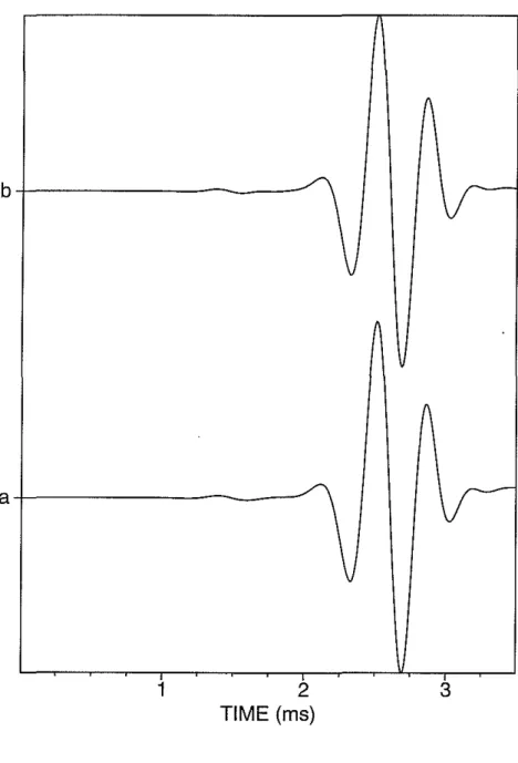
To demonstrate this decomposition we first consider the isotropic formation. The parameters of the formation are listed in Table1. Itis a slow formation. The water-filled borehole is 10 cm in radius. The source is a Kelly wavelet at center frequency 2 kHz. The source and the receiver are located at the center of the borehole. The source and receiver separation is 2 meters. These parameters are kept the same in the paper. The comparison of the direct finite difference computation with the projection of Eq. (4) is plotted in Figure 1. The dipole source is at an azimuthal angle of 45 degrees. The projected and the computed waveforms are in excellent agreement.

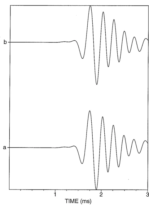
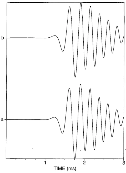
The elastic constants of the TI formations are listed in Table 2. Two types of TI formation are considered: (1) Bakken shale, a fast formation; and (2) Austin chalk, a slow formation. The symmetry axis of the TI formation is perpendicular to the borehole axis. For the dipole source at an azimuthal angel of 45 degrees, the comparisons of direct-computed waveforms with the projected one are plotted in Figures 2 and 3 for the measurement in theX and the Y direction, respectively. The formation used is Bakken shale. Once again they are in excellent agreement. Equations (4) and (5) permit the decomposition of the dipole source into the principal directions and the computation of the response in the principal directions. This can save computing time for the acoustic dipole log simulation in an anisotropic formation with different azimuthal directions.

From two inline dipole measurements along the X and the Y axis, the inline and crossline dipole measurements at azimuthal angle

g

can be easy obtained from the projection. We have:

B B g B ' g

vinline = Vxcos

+

VySIn and

B 0 •

g

B

g

Vcrossline = _-VxSIn

+

V_ycos .

Substituting Eqs. (4) and (5) into the above equations we obtain:

B 2g+ '2g

vinline = Vxcos VySIn and

V~rossline

=

(-V

x

+

vy )sin

e

cos

e.

(6)

(7)

(8)

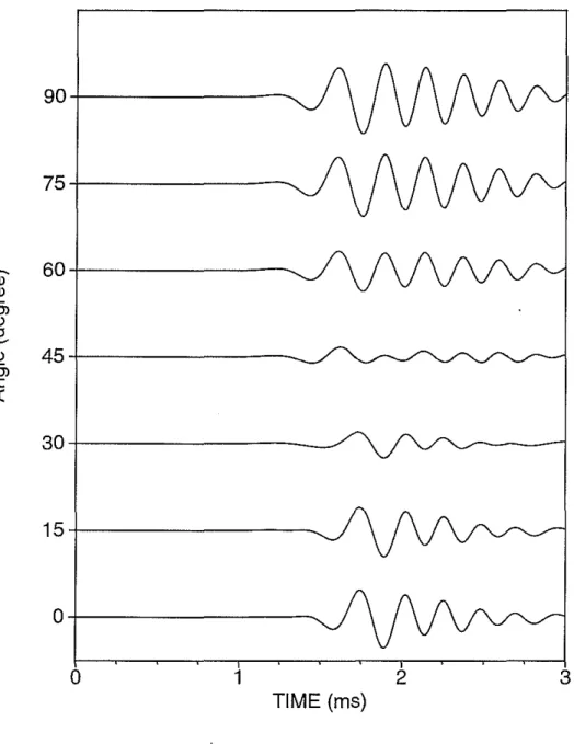
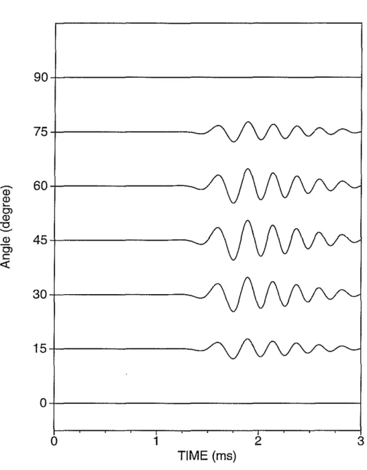
(9) The same equations are also given by Sinha et al. (1994) and Esmersoy et al. (1994). These are our forward decomposition formulas for the acoustic dipole log. To show some examples, we projected the inline and the crossline dipole logs in Bakken shale and Austin chalk formations at different azimuthal angles. The waveforms are plot-ted in Figures 4, 5, 6 and 7. In isotropic formations the crossline dipole log is zero. In anisotropic formations the crossline dipole vanishes only when the dipole source is aligned with the symmetry axis. Generally, the crossline dipole log is not zero. In logging data processing, the crossline dipole log can be used to determine whether the formation shear wave velocity is anisotropic and the direction of the principal axis of

(10) the anisotropy. In inline dipole logs (Figures 4 and 6), it is clear from the waveforms that at a 90 degree azimuthal angle, the arrival times are earlier than at 0 degrees. This is the reflection of the shear wave velocity azimuthally dependent. The inline dipole log can provide the measurements of anisotropy from the arrival time differences between different azimuthal angles.

PARTICLE MOTION AND POLARIZATION ANALYSIS

Shear wave splitting is often observed from teleseismic events. The particle motion of a shear wave is polarized along the principal directions. Ifthe acoustic dipole log in the anisotropic formation is also polarized along the principal directions, then we can find the principal direction from the polarization analysis. This will make it easy to solve the inverse decomposition question.

We define the mean value ofN observations of variable x(i) as (Kanasewich, 1981)

1 N

E(x) = N Lx(i)

i=l

and the covariance between two variables XI and X2 as 1 N

COV[XI,X2]

=

N L(xI(i) - E(xI))((X2(i) - E(X2)).

i=l

(11)

For the two components of the dipole log (v"' vy), the covariance matrix C can be formed as

C

= (

Cov[v", v,,] Cov[v", vy] ) (12)

Cov[v", vy] Cov[vy, vy]

If Al and A2 are the eigenvalues of the covariance matrix C and Al

>

A2, then the quantity

A2

P

=

1- - (13)

Al

estimates the rectilinearity of the particle motion. When the rectilinearity is high (AI»

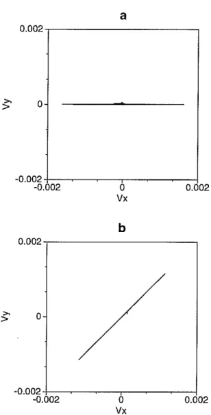
A2) the particle motion is close to the linear polarization. When the rectilinearity is near zero (AI co: A2) the particle motion is near circular. The direction of polarization may be measured by considering the eigenvector associated with the largest eigenvalue. First, we consider the particle-motion of the dipole log in the isotropic formation. The synthetic particle motion of the dipole log is plotted in Figure 8. The particle motion is shown in the X-Y plane. Figure 8(a) shows the direction of the dipole source to be along the X axis. Figure 8(b) shows the dipole source at an azimuthal angel of 45 degrees. Without further analysis the plot demonstrates that the dipole log in an isotropic formation is linearly polarized along the source direction. This is very easy to understand. In isotropic formations the only preferred direction is the source direction.

TI formations are considered next. The formation shear wave velocity is azimuthally dependent. The particle motions are plotted in Figure 9 for Bakken shale and in Figure 10 for Austin chalk. From the particle motion plots in both formations, the linear polarizations at azimuthal angles of 0 and 90 degrees are easy to understand. The symmetry of the model requires that there is no motion perpendicular to the plane of the symmetry (Gxy = Gyx = 0). The linearly polarized particle motions at azimuthal angles of 0 and 90 degrees also give some indirect accuracy measure of the finite difference method. When the dipole source is not aligned with the principal axis of the formation, we would intuitively expect that it will be polarized along the two principal axes. But the plots of the particle motion did not show these polarizations clearly. The reason is that our intuition is based on the far-field shear body waves in anisotropic media. The dipole log is using a flexural wave which is a guided mode and the acoustic logging distance belongs to the near field. In general, for one period of separation in the time domain, it takes the distance of a wavelength divided by the percent of anisotropy. For example, a 5% anisotropy takes about 20 wavelengthes to get one period separation in time.

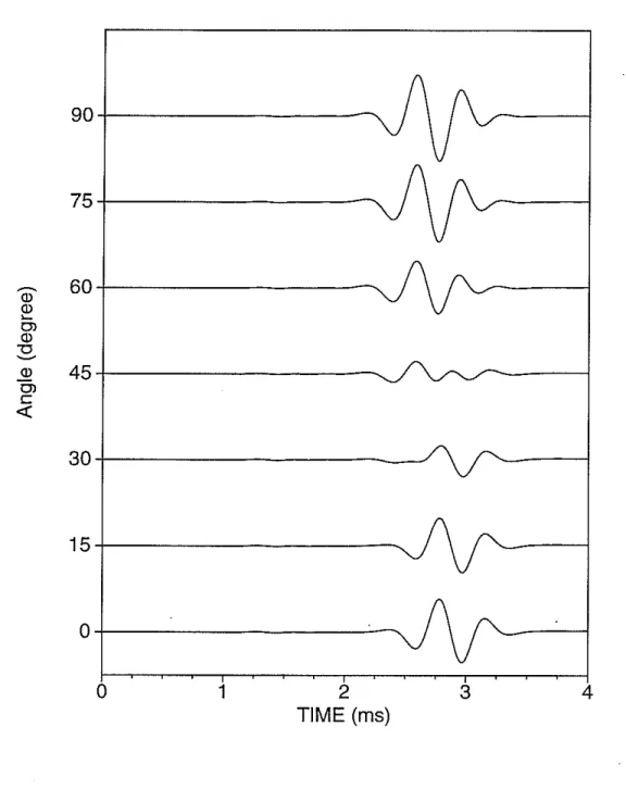
In order to verify the distance effect, we increase the source and receiver distance to 4.5 meters in the Austin chalk formation to do the finite difference calculations. Other parameters are not changed. The inline and crossline dipole logs are plotted in Figures 11 and 12. The arrival times at azimuthal angles of 0 and 90 degrees are obviously more separated than the 2 meter case (Figure 6). The particle motion is plotted in Figure 13. Itis very clear from the plot that the particle motion begins in the fast shear wave direction. This example confirms that no clear polarized particle motion in the dipole log is due to the nature of near-field logging.

The rectilinearity analysis of the dipole particle motion in Bakken shale and Austin chalk are listed in Table 3. At azimuthal angles of 0 and 90 degrees, the particle motion is linearly polarized. The particle motion with a source at an arbitrary azimuthal angle did not show any particular patterns. The particle motion pattern depends on the relative phase of the Green's fuilction Gxx and Gyy . This phase depends on the source receiver distance, the degree of anisotropy and the frequency. From the particle motion analysis we only see that the initial particle motion is directed along the fast shear wave direction with a large source receiver separation. But, due to the near field nature of acoustic logging, this initial particle motion is hard to obtain accurately for any practical use. In order to answer the final question we have to seek another way to do the inverse decomposition.

INVERSE DECOMPOSITION OF THE DIPOLE LOG

In field logging situations, we do not know the principal direction of the formation. The inverse problem is how to find the principal direction from the measurement at an arbi-trary azimuthal angle. We assume two pairs of inline and crossline dipole measurements are collected in perpendicular directions. The measured data is represented as a data

vector V

=

(V(tl), V(t2), ... , v(tn)jT. The two inline dipole measurements are Vft and Vf/90 The two crossline dipole measurements areV~l andV~t90. The problem is how to find the azimuthal angle

e

and the inline measurements along the X and the Y axis from these four data vectors. By using Eqs. (8) and (9) we have:

Vfl Vxcos2e+Vysin2e (14)

Vfro = V x sin2e+ vycos2e (15)

V~l (-Vx + V y) sine cos

e

(16)

v~ro (Vx - V y) sine cos

e.

(17)

Equation (17) is not an independent one, because V~l

= -

V~t90 This leaves us with three equations with three unknowns. The three unknowns are angle

e,

Vx and V y. With a few algebra manipulations of Eqs. (14), (15) and (16) we obtain:

V~l(tan

e-

cot

e)

Vfl - V~+90 (18)

V x = Vfl-V~ltane (19)

V y V~+9o+V~ltane. (20)

Notice that Eq. (18) contains n equations, where n is the number of measurements. So angle

e

is overdetermined. We seek the least-square solution for

e.

This solution is given below:

(VO

jT .

(VO _ V O+90 ) tan2_{e - cl}

il il tane-1 = 0 (21)

(V~I)T .V~l .

e

can be easily obtained by finding the root of the second-order polynomial. Once

e

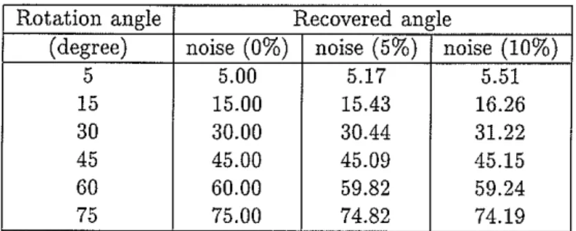
is known, V x and V y can be calculated directly from Eqs. (19) and (20). So the inverse decomposition is given by the analytical expressions in the least-square sense.

Next, we consider a numerical example. Austin chalk formation is considered once again. First, we determine the rotated angle

e

by using Eq. (21). The inline and crossline dipole logs are obtained by using Eqs. (8) and (9). These data are then used to recover the rotated angle. Random noise is added to the inline and crossline data to test the sensitivity of the formula to noise. The recovered angles are listed in Table 4: Ifthere is no noise added to the data, the rotated angles are recovered almost exactly. With 5% noise the differences between the recovered angle and the actual rotated angle are less than 0.5 degree. When the noise level s increased to 10%, the differences are less than 1.5 degrees. Under the noise condition the inverse decomposition formula can still give a very good estimation of the principal direction. Recovered waveforms along the principal directions are plotted in Figures 14 and 15. The inline and crossline logging data. at azimuthal angles of30 and 120 degrees are used. The inline and crossline waveform at azimuthal angle30 can be found in Figure 6 and 7. The four traces shown in the plots are original data, recovered from noise-free, 5% noise, and 10% noise data. The waveforms along the principal directions are recovered very well even under noisy conditions. The inverse decomposition formulas are very computationally efficient. They can be used to process field acoustic logging data in anisotropic formations.

CONCLUSIONS

In this paper, analytic expressions are obtained for both forward and inverse decompo-sition of acoustic dipole logging data. These decompodecompo-sition formulas are valid because the principal of superposition holds for linear wave propagation in anisotropic media. These very simple analytic formulas can be directly applied to field logging data process-ing. Synthetic acoustic dipole logs are used to demonstrate these forward and inverse decompositions. The synthetics are calculated by the 3-D finite difference method. The numerical examples show that the inverse decomposition formula works very well with noisy data. The particle motion of the dipole log in an anisotropic formation is com-plicated. This is because the acoustic logging distance is in the near field. The particle motion with a dipole source aligned with the principal direction is linearly polarized. When the dipole source is at an arbitrary azimuthal angle, the initial particle motion tends to point to the fast shear wave direction. But this initial polarization can only have very limited use in field data situations.

ACKNOWLEDGMENTS

This research was supported by the Borehole Acoustics and Logging Consortium at ERL and by the ERL/nCUBE Geophysical Center for Parallel Processing. One author (N.C.) was partly supported by Los Alamos National Laboratory as a postdoctoral fellow.

REFERENCES

Barton, C.A. and Zoback, M.D., 1988, Determination of in situ-stress orientation from borehole guided waves, J. Geophys. Res., 93. 7834-7844.

Chan, A.K. and Tsang, L., 1983, Propagation of acoustic waves in a fluid-filled borehole surrounded by a concentrically layered transversely isotropic formation, J. Acoust. Soc. Am., 74, 1605-1616.

Cheng, N., Cheng, C.H., and Toksoz, M.N., 1995, Borehole wave propagation in three-dimension, to appear in J. Acoust. Soc. Am.

Ellefsen, KJ., 1990, Elastic wave propagation along a borehole in an anisotropic medium, Ph.D. Thesis, Massachusetts Institute of Technology, Cambridge, MA.

Esmersoy, C., Koster, K., Williams, M., Boyd, A., and Kane, M., 1994, Dipole shear anisotropy logging, 64th S.E. G. Annual Meetin9 Expanded Abstract, Los Angeles, CA.

Higdon, R.L., 1990, Radiation boundary conditions for elastic wave propagation, SIAM

J. Numer. Anal., 27, 831-870.

Kanasewich, E.R., 1981, Time Sequence Analysis in Geophysics, The University of Al-berta Press, Third Edition.

Leslie, H.D. and Randall, C. T., 1992, Multipole sources in boreholes penetrating anisotropic formations: Numerical and experimental results, J. Acoust. Soc. Am., 91, 12-27. Leveille, J.P. and Seriff, A.J., 1989, Borehole wave particle motion in anisotropic

for-mations, J. Geophys. Res., 94, 7183-7188.

Sinha, RK, Norris, A.N. and Chang, S.K, 1994, Borehole flexural modes in anisotropic formations, Geophysics, 59, 1037-1052.

White, J.E. and Tongtaow, C., 1981, Cylindrical waves in transversely isotropic media, J. Acoust. Soc. Am. 70, 1147-1155.

Quantity Value

Vp 2770 mjs Vs 1219 mjs p 2250 kgjm3

Table 1: Elastic properties of the isotropic formation.

Quantity Bakken shale Austin chalk

Cn

40.9 GPa 22.0 GPa C12 10.3 GPa 15.8 GPa C13 8.5 GPa 12.0 GPa C33 26.9 GPa 14.0 GPa C44 10.5 GPa 2.4 GPa p 2230 kgjm3 _{2200 kgjm}3

Table 2: Elastic properties of transversely isotropic formations, which represent Bakken shale and Austin chalk (Sinha et al., 1994).

Source direction Rectilinearity

(degree) shale (2m) chalk (2m) chalk (4.5m)

0 1.00 1.00 1.00 15 0.98 0.97 0.95 30 0.95 0.93 0.83 45 0.96 0.93 0.75 60 0.98 0.96 0.84 75 0.99 0.99 0.95 90 1.00 1.00 1.00

Table 3: Polarization analysis of the dipole log. The formations are Bakken shale and Austin chalk. The source-receiver separations are 2 and 4.5 meters.

Rotation angle Recovered angle

(degree) noise (0%) noise (5%) noise (10%)

5 5.00 5.17 5.51 15 15.00 15.43 16.26 30 30.00 30.44 31.22 45 45.00 45.09 45.15 60 60.00 59.82 59.24 75 75.00 74.82 74.19

Table 4: Recovered rotation angle from inline and crossline data. Random noise is added to the data.

b

a

fI

'\

V

fI

\

V

,

,

1

2

TIME

(ms)

3

Figure 1: Comparison of the finite difference synthetic with linear decomposition in isotropic formation. The dipole source is at azimuthal angle of 45 degrees. The wave-form in the X direction is shown. Trace (a) finite difference synthetic. Trace (b) decomposition according to Equation (4).

b

a

11 A 1\

\IV

\

V

r

A

Vv

\

v

1

TIME

(ms)

2

3

Figure 2: Comparison of the finite difference synthetic with linear decomposition in Bakken shale TI formation. The dipole source is at azimuthal angle of 45 degrees. The waveform in the X direction is shown. Trace (a) finite difference synthetic. Trace (b) decomposition according to Equation (4).

b

a

II

(\

V

V

V

II II

Iv

V

rv

1

TIME

(ms)

2

3

Figure 3: Comparison of the finite difference synthetic with linear decomposition in Bakken shale TI formation. The dipole source is at azimuthal angle of 45 degrees. The waveform in the Y direction is shown. Trace (a) finite difference synthetic. Trace (b) decomposition according to Equation (5).

90

+---..,.

75

+---____...

~

60

OJ OJ ~ 0) OJ -0 ~ ~

45

0) c

«

30

15

+---___..

0 + - - - . . .

o

1

TIME

(ms)

2

3

Figure 4: Projected inline dipole log in Bakken shale formation at different azimuthal angles by using Equation (8).

9 0 + - - - 1

7 5 + - - - /

~

60

Q) Q) ~ 0 ) Q) "0 ~ Q)

45

0 ) c <J::

30

15

+ - - - . /

0 + - - - 1

o

1

TIME

(ms)

2

3

Figure 5: Projected crossline dipole log in Bakken shale formation at different azimuthal angles by using Equation (9).

90 - 1 - - - _ _ _ .

75

- 1 - - - .

~

60

Q) Q) ~ Ol Q) "0 ~ .S!!

45

Ol c

«

30

15

- 1 - - - . .

0-1---'---o

1

2

TIME

(ms)

3

4

Figure 6: Projected inline dipole log in Austin chalk formation at different azimuthal angles by using Equation (8).

9 0 + - - - j

75 - + - - - . . . J

~

60

Ql Ql ~ Ol Ql ""0 ~ Ql

45

Ol c::

«

30

1 5 + - - - . . . . /

O + - - - j

o

1

2

TIME

(ms)

3

4

Figure 7: Projected crossline dipole log in Austin chalk formation at different azimuthal angles by using Equation (9).

a 0 . 0 0 2 , - - - ,

S'

0 -0.002 -0.002 0 0.002 Vx

b

0.002

S'

0 0.002

o

Vx -0.002+--~--_,..----_l -0.002

Figure 8: X-Y plane particle motion of dipole log in isotropic formation. (a) dipole source along the X axis. (b) dipole source at the azimuthal angle of 45 degrees.

a b 0.002 - , - - - ' - ; 0 . 0 0 2 , - - - , o o -0.002 -0.002 -0.002 0 0.002 -0.002 0 0.002 Vx Vx c d 0.002 0.002 o o -0.002+:-:,----.---,---::-:1 -0.002

+:c----,---::-:I

-0.002 0 0.002 -0.002 0 0.002 ~ ~

Figure 9: X-Y plane particle motion of dipole log in Bakken shale formation. The azimuthal angle of the dipole source is (a) O. (b) 15. (c) 30. (d) 45. (e) 60. (f) 75. (g)

e

0 . 0 0 2 , - - - , f 0 . 0 0 2 , - - - , o o -0.002

t:c::---r----:-J

-0.002

t:c::---r----:-J

-0.002 0 0.002 -0.002 0 0.002 Vx Vx 9 0 . 0 0 2 - , - - - ,

5:

0 -0.002

t:c::---,---:-J

-0.002 0 0.002 Vx Figure 9: continued

a b 0 . 0 0 2 , - - - , 0 . 0 0 2 , - - - , o o -0.002 -0.002 -0.002 0 0.002 -0.002 0 0.002 Vx Vx c d 0.002 0.002 o o -0.002+---~----_j -0.002

+:c,.---,---,:-:!

-0.002 0 0.002 -0.002 0 0.002 ~ ~

Figure 10: X-Y plane particle motion of dipole log in Austin chalk formation. The azimuthal angle of the dipole source is (a) O. (b) 15. (c) 30. (d) 45. (e) 60. (f) 75. (g)

e

f o 0 . 0 0 2 - , - - - , o 0 . 0 0 2 - , - - - , 0.002 o Vx ·0.002+---~--- _ __I ·0.002+-- ~--"--_-_1 ·0.002 0 0.002 ·0.002 Vx 9 0 . 0 0 2 - , - - - _ - - - ,

5:'

0 · 0 . 0 0 2 t : e : - - - - + - - - _ _ , : - : ! ·0.002 0 0.002 Vx Figure 10: continued

6

4

2

o

O..j---~

9 0 . . j - - - . ,

7 5 . . j - - - . ,

1 5 . . j

-~

60

OJ OJ ~ OJ OJ "Cl ~ 45 OJ 0:> c:

«

30

TIME

(ms)

Figure 11: Projected inline dipole log in Austin chalk formation at different azimuthal angles by using Equation (8). The source-receiver distance is 4.5 meters.

6

4

2

o

0 - 1 - - - 1

9 0 - 1 - - - 1

75- 1 - - - / 15

- 1 - - - . /

~

60

CD CD ~ OJ CD -0 ~

45

CD C> c

«

30

TIME

(ms)

Figure12: Projected crossline dipole log in Austin chalk formation at different azimuthal angles by using Equation (9). The source-receiver distance is 4.5 meters.

a b 0 . 0 0 2 , - - - , 0 . 0 0 2 , - - - , o o -0.002 -0.002 -0.002 0 0.002 -0.002 0 0.002 Vx Vx

c

d 0.002 0.002 o o -0.002+---~----_I -0.002

-1-:-::---,---,:-:1

-0.002 0 0.002 -0.002 0 0.002 Vx ~

Figure 13: X-Y plane particle motion of dipole log in Austin chalk formation. The source-receiver distance is 4.5 meters. The azimuthal angle of the dipole source is (a) O. (b) 15. (c) 30. (d) 45. (e) 60. (f) 75. (g) 90.

e 0 . 0 0 2 , - - - , f 0 . 0 0 2 , - - - ,

,.,

₀ ~ 0

(

\

>

lJ

-0.002 -0.002 -0.002 0 0.002 -0.002 0 0.002 Vx Vx 9 0.002 ~ 0 -0.002

+:::---,:---,:-:1

-0.002 0 0.002 Vx Figure 13: continued

4

3

2

TIME

(ms)

1

o

b - l - - - . . . - - ,

a-t---,

Figure 14: Recovered waveforms along the X axis from 30 and 120 degrees inline and crossline dipole logs. The formation is Austin chalk. Trace (a) original waveform along the X axis. Trace (b) recovered from data without noise. Trace (c) recovered from data with 5% random noise. Trace (d) recovered from data with 10% random noise.

b - t - - - . . . . - - ,

a+----,---,

o

1

2

TIME (ms)

3

4

Figure 15: Recovered waveforms along the Y axis from 30 and 120 degrees inline and crossline dipole logs. The formation is Austin chalk. Trace (a) original waveform along the Y axis. Trace (b) recovered from data without noise. Trace (c) recovered from data with 5% random noise. Trace (d) recovered from data with 10% random noise.